HAL Id: hal-00650235
https://hal.archives-ouvertes.fr/hal-00650235v2
Submitted on 20 Nov 2012
HAL is a multi-disciplinary open access
archive for the deposit and dissemination of
sci-entific research documents, whether they are
pub-lished or not. The documents may come from
teaching and research institutions in France or
abroad, or from public or private research centers.
L’archive ouverte pluridisciplinaire HAL, est
destinée au dépôt et à la diffusion de documents
scientifiques de niveau recherche, publiés ou non,
émanant des établissements d’enseignement et de
recherche français ou étrangers, des laboratoires
publics ou privés.
Divergence Analysis with Affine Constraints
Diogo Sampaio, Rafael Martins, Sylvain Collange, Fernando Magno Quintão
Pereira
To cite this version:
Diogo Sampaio, Rafael Martins, Sylvain Collange, Fernando Magno Quintão Pereira. Divergence
Analysis with Affine Constraints. 24th International Symposium on Computer Architecture and
High Performance Computing, Oct 2012, New-York, NY, United States. pp.67-74,
�10.1109/SBAC-PAD.2012.22�. �hal-00650235v2�
Divergence Analysis with Affine Constraints
∗
Diogo Sampaio
Rafael Martins
Sylvain Collange
Fernando Magno Quint˜
ao Pereira
Departamento de Ciˆ
encia da Computa¸c˜
ao
Universidade Federal de Minas Gerais, Brazil
{sampaio,rafaelms,sylvain.collange,fernando}@dcc.ufmg.br
June 26, 2012
Abstract
The rising popularity of graphics processing units is bringing renewed interest in code optimization tech-niques for SIMD processors. Many of these optimiza-tions rely on divergence analyses, which classify vari-ables as uniform, if they have the same value on every thread, or divergent, if they might not. This paper introduces a new kind of divergence analysis, that is able to represent variables as affine functions of thread identifiers. We have implemented this analy-sis in Ocelot, an open source compiler, and use it to analyze a suite of 177 CUDA kernels from well-known benchmarks. We can mark about one fourth of all program variables as affine functions of thread identi-fiers. In addition to the novel divergence analysis, we also introduce the notion of a divergence aware reg-ister allocator. This allocator uses information from our analysis to either rematerialize affine variables, or to move uniform variables to shared memory. As a testimony of its effectiveness, our divergence aware allocator produces GPU code that is 29.70% faster than the code produced by Ocelot’s register allocator. Divergence analysis with affine constraints is publicly available in the Ocelot compiler since June/2012.
1
Introduction
Increasing programmability and low hardware cost are boosting the use of graphical processing units (GPU) as tools to run high-performance applications. In these processors, threads are organized in groups, called warps, that execute in lock-step. To better un-derstand the rules that govern threads in the same warp, we can imagine that each warp has simulta-neous access to a number of processing units, but
∗This work was partially supported by CNPq, CAPES and
FAPEMIG.
uses only one instruction fetcher. As an example, if a warp groups 32 threads together, then it can pro-cess simultaneously 32 instances of the same instruc-tion. Regular applications, such as scalar vector mul-tiplication, fare very well in GPUs, because we have the same operation being independently performed on different data. However, divergences may happen in less regular applications whenever threads inside the same warp follow different paths after conditional branches. The branching condition might be true to some threads, and false to others. Given that each warp has access to only one instruction at each time, in face of a divergence some threads will be idle while others execute. Hence, divergences may be a major source of performance degradation – a loss that is hard to overcome. Difficulties happen because find-ing highly divergent branches burdens the application developer with a tedious task, which requires under-standing code that might be large and complex.
In this paper we introduce a new divergence anal-ysis, i.e., a technique that identifies variable names holding the same value for all the threads in a warp. We call these variables uniform. We improve on pre-vious divergence analyses [1, 2, 3, 4] in non-trivial ways. In Section 3, we show that our analysis finds not only uniform variables, but also variables that are affine functions of thread identifiers. Contrary to Aiken’s approach [1], we work on SIMD machines; thus, we handle CUDA and OpenCL programs. By taking affine relations between variables into consid-eration, we also improve on Stratton’s [4], Karren-berg’s [3] and Coutinho’s [2] techniques.
The problem of discovering uniform variables is important in different ways. Firstly, it helps the compiler to optimize the translation of SIMD lan-guages, such as C for CUDA and OpenCL, to ordi-nary CPUs. Currently there exist many attempts to compile such languages to ordinary CPUs [5, 3, 4]. Vector instruction sets such as the x86’s SSE
exten-sion do not support divergences natively. Thus, com-pilers might produce very inefficient code to handle this phenomenon at the software level. This burden can be safely removed from non-divergent branches. Secondly, our analysis enables divergence aware code optimizations, such as Coutinho et al.’s [2] branch fusion, and Zhang et al.’s [6] thread reallocation. In this paper, we augment this family of techniques with a divergence aware register allocator. As we will show in Section 4, we use divergence information to decide the best location of variables that have been spilled during register allocation. Our affine analysis is spe-cially useful to this optimization, because it allows us to perform register rematerialization [7] in SIMD processing elements.
Our novel divergence analysis and register allocator are, since June 2012, distributed under GPL license as part of the Ocelot compiler [5]. We have compiled 177 CUDA kernels from 46 applications taken from the Rodinia [8] and the NVIDIA SDK publicly avail-able benchmarks. In practice our divergence analysis runs in linear time on the number of variables in the source program. The experiments also show that our analysis is more precise than Ocelot’s previous diver-gence analysis, which was based on Coutinho et al.’s work [2]. We not only point that about one fourth of the divergent variables are affine functions of thread IDs, but also find 4% more uniform variables. Fi-nally, our divergence aware register allocator is ef-fective: we speedup the code produced by Ocelot’s linear scan register allocator by almost 30%.
2
Divergences in one Example
In order to describe our analysis and optimizations, we will be working on top of µ-Simd, a core SIMD lan-guage whose operational semantics has been defined by Coutinho et al. [2]. Figure 1 gives the syntax of this language. The execution of a µ-Simd program consists of a number of processing elements (PE) which execute in lock-step. A program P contains a set of variable names V , and each PE has access to a mapping θ : V 7→ N. Each PE sees the same set of variable names, yet these names are mapped into different address spaces. The special variable Tid, the thread identifier, holds a unique value for each PE. An assignment such as v1= v2+ c causes each active PE to compute – simultaneously – the value of θ[v2] + c, and to use this result to update θ[v1]. Threads com-municate through a shared memory Σ, accessed via load and store instructions. For instance, when
pro-Labels ::= l ⊂ N
Constants (C) ::= c ⊂ N
Variables (V ) ::= tid∪ {v1, v2, . . .}
Operands (V ∪ C) ::= {o1, o2, . . .}
Instructions ::=
– (jump if zero/not zero) | bz/bnz v, l
– (unconditional jump) | jumpl
– (store into shared memory) | ↑ vx= v
– (load from shared memory) | v =↓ vx
– (atomic increment) | v←a− vx+ c
– (binary addition) | v1= o1+ o2
– (binary multiplication) | v1= o1× o2
– (general binary operation) | v1= o1⊕ o2
– (general unary operation) | v = ⊕o
– (simple copy) | v = o
– (synchronization barrier) | sync
– (halt execution) | stop
Figure 1: The syntax of µ-Simd instructions.
cessing ↑ vx= v, the active PEs performs the assign-ment Σ[θ[vx]] = v simultaneously. Inversely, v =↓ vx updates θ[v] with the value in Σ[θ[vx]]. The language provides mutual exclusion via the atomic increment v ←− va x+ c, which, for some arbitrary serialization of the active PEs, reads Σ[θ[vx]], increments it by c, stores the incremented value back at Σ[θ[vx]] and uses the modified value to update θ[v].
Figure 2(Top) shows an example of a program writ-ten in µ-Simd that sums up the columns of a triangu-lar matrix. However, only the odd indices in each col-umn contribute to the sum, as we ensure with the test at labels l7 and l8. In this program threads perform different amounts of work: the PE that has Tid = n visits n + 1 cells. After a thread leaves the loop, it must wait for the others. Processing resumes once all of them synchronize at label l15. At this point, each thread sees a different value stored at its image of variable d, which has been incremented Tid+ 1 times. Hence, we say that d is a divergent variable outside the loop. Inside the loop, d is uniform, because ev-ery active thread sees the same value stored at that location. Consequently, the threads active inside the loop take the same path at the branch in label l8.
A conditional test bnz v, l′ at label l causes all the threads to evaluate their θ[v]. Those that find θ[v] 6= 0 branch to l′, whereas the others fall through the next instruction at l + 1. If two threads take different paths, i.e., v is divergent, then we say that the threads diverge at l. Figure 2(Bottom) illustrates this phenomenon via a snapshot of the execution of our example program. Our running program contains four threads: t0, . . . , t3. When visiting the branch at label l6 for the second time, the predicate p is 0 for thread t0, and 1 for the other PEs. In face of this di-vergence, t0is pushed onto a stack of waiting threads, 2
l7: p = d % 2 bnz p, l11 l15: sync x= d ! 1 "x= s stop l0: s = 0 d = 0 i = tid x = tid + 1 L = c # x l5: p = i ! L bz p, l15 l9: x= $i s = s + x l11: sync d = d + 1 i = i + c jmp l5 Cycle Instruction t0 t1 t2 t3 14 l5: p = i − L X X X X 15 l6: bz p, l15 X X X X 16 l7: p = i % 2 • X X X 17 l8: bz p, l11 • X X X . . . 25 l6: bz p, l15 • X X X 26 l7: p = i % 2 • • X X 27 l8: bz p, l11 • • X X . . . 44 l5: bz p, l15 • • • X 45 l15: sync X X X X
Figure 2: (Top) A µ-Simd program. (Bottom) An execution trace of the program. If a thread t executes an instruction at cycle j, we mark the entry (t, j) with the symbol X. Otherwise, we mark it with •.
while the other threads continue executing the loop. When the branch is visited a third time, a new diver-gence will happen, this time causing t1 to be stacked for later execution. This pattern will happen once again with thread t2, although we do not show it in Figure 2. Once t3 leaves the loop, all the threads synchronize via the sync instruction at label l15, and resume lock-step execution.
3
The Analysis
Gated Single Static Assignment Form. To
in-crease the precision of our analysis, we convert pro-grams to the Gated Static Single Assignment form [9, 10] (GSA). This program representation uses three special instructions: µ, γ and η functions, defined as follows: γ functions represent the joining point of dif-ferent paths created by an “if-then-else” branch in
the source program. The instruction v = γ(p, o1, o2) denotes v = o1 if p, and v = o2 if ¬p; µ functions, which only exist at loop headers, merge initial and loop-carried values. The instruction v = µ(o1, o2) represents the assignment v = o1 in the first itera-tion of the loop, and v = o2in the others; η functions represent values that leave a loop. The instruction v= η(p, o) denotes the value of o assigned in the last iteration of this loop, which is controlled by the pred-icate p. Figure 3 shows the GSA version of the pro-gram in Figure 2. This format serves us well because it separates variables into different names, which we can classify independently as divergent or uniform, while taking control dependences into consideration. We use Tu and Padua’s [10] almost linear time algorithm to convert a program into GSA form. Ac-cording to this algorithm, γ and η functions exist at the post-dominator of the branch that controls them. A label lp post-dominates another label l if every path from l to the end of the program goes through lp. Fung et al. [11] have shown that re-converging divergent PEs at the immediate post-dominator of the divergent branch is nearly optimal with respect
to maximizing hardware utilization. Thus, we
assume that each γ or η function encodes an implicit synchronization barrier, and omit the sync instruc-tion from labels where these funcinstruc-tions appear. We use Appel’s parallel copy semantics [12] to evaluate these functions. For instance, the µ assignment at l5, in Figure 3 denotes two parallel copies: either we perform [i1,sum1, d1] = (i0,sum0, d0), in case we are entering the loop for the first time, or we do [i1,sum1, d1] = (i2,sum3, d2) otherwise.
Affine Analysis. The objective of the divergence
analysis with affine constraints is to associate with every program variable an abstract state which tells us if that variable is uniform, divergent or affine, a term that we shall define soon. This abstract state is a point in a lattice A, which is the product of two instances of a simpler lattice C, e.g., A = C × C. We let C be the lattice formed by the set of integers
Z augmented with a top element ⊤ and a bottom
element ⊥, plus a meet operator ∧, such that c1∧c2= ⊥ if c16= c2, and c∧c = c. Notice that C is the lattice used in the compiler optimization known as constant propagation; hence, for a proof of monotonicity, see Aho et al [13, p.633-635]. If (a1, a2) are elements of A, we represent them using the notation a1Tid+ a2. We define the meet operator of A as follows:
l8: p1 = d1 % 2 bnz p1, l12 l16: [s4, d3] = ![p0, (s1, d1)] x3 = d3 " 1 #x3 = s4 stop l0: s0 = 0 d0 = 0 i0 = tid x0 = tid + 1 L0 = c $ x0 l5:[i1,s1,d1] = µ[(i0, s0 ,d0),(i2, s3, d2)] p0 = i1 " L0 bz p0, l16 l10: x2 = %i1 s2 = s1 + x2 l12: [s3] = &(p1, s2, s1) d2 = d1 + 1 i2 = i1 + c jmp l5
Figure 3: The program from Figure 2 converted into GSA form.
We let the constraint variable JvK = a1Tid+a2denote the abstract state associated with variable v. We determine the set of divergent variables in a µ-Simd program P via the constraint system seen in Figure 4. Initially we let JvK = (⊤, ⊤) for every v defined in the text of P , and JcK = (0, c) for each c ∈ Z.
Complexity. The constraint system in Figure 4 can be solved in time linear on the size of the program’s
dependence graph [14]. The dependence graph has
a node for each program variable. If the constraint that produces JvK uses Jv′K as a premise, then the dependence graph contains an edge from v′ to v. As an example, Figure 5 shows the program dependence graph that we have extracted from Figure 3. We show only the dependence relations in the program slice that contributes to create variable d3. Each node in Figure 5 has been augmented with the results of our divergence analysis with affine constraints.
Correctness. Given a µ-Simd program P , plus
a variable v ∈ P , we say that v is uniform if ev-ery processing element always sees v with the same value at simultaneous execution cycles. On the other hand, if these processing elements see v as the same affine function of their thread identifiers, e.g., v = c1Tid + c2, c1, c2 ∈ Z, then we say that v is affine. Otherwise, if v is neither uniform nor affine, then we call it divergent. The abstract state of each variable tells us if the variable is uniform, affine or divergent.
Theorem 3.1 If JvK = 0Tid + a, a ∈ C, then v is uniform. If JvK = cTid+ a, a ∈ C, c ∈ Z, c 6= 0, then v is affine. d0 d1 d2 µ + ! d3 p0 L0 i1 " c x0 tid + i0 i2 0 # µ + 1 (0, 0) (0, 1) (1, 0) (1, !) (1, !) (0, !) (1, 0) (1, 1) (!, !) (!, !) (!, !) (0, 0) (0, !) (0, !) p1 (0, !)
Figure 5: The dependence graph denoting the slice of the program in Figure 3 that produces variable d3. The figure shows the results of our divergence analysis with affine constraints.
4
Register Allocation
Register allocation is the problem of finding storage location to the values manipulated in a program. Ei-ther we place these values in registers or in memory. Values mapped to memory are called spills. A mod-ern GPU has many memory levels that the compiler must take into consideration when trying to decide where to place spills. Traditional register allocators, such as the one used in the NVIDIA compiler, or in Ocelot [5], map spills to the local memory. This mem-ory is exclusive to each thread, and is located off-chip in all the architectures that we are aware off. We have observed that spilled values that our analysis classi-fies as uniform or affine can be shared among all the threads in the same warp. This observation is par-ticularly useful in the context of graphics processing units, because they are equipped with a fast-access sharedmemory, which is visible to all the threads in execution. The main advantage of mapping spills to the shared memory is speed. This memory is approx-imately 100x faster than the local memory [15].
We have developed a set of rewriting rules that can be applied after register allocation, mapping some of the spills to the shared memory. To accommodate the notion of local memory in µ-Simd, we have aug-mented its syntax with two new instructions: v =⇓ vx loads the value stored at local memory address vx into v; ⇑ vx = v stores v into the local memory ad-dress vx. The table in Figure 6 shows our rewriting rules. In row (ii) we are simply remapping uniform variables from the local to the shared memory. The affine analysis sometimes lets us perform constant 4
v = c × Tid [TidA] JvK = cTid+ 0 v = v′ [AsgA] JvK = Jv′K
v←a− vx+ c [AtmA] JvK = ⊥Tid+ ⊥ v = c [CntA] JvK = 0Tid+ c
v = ⊕o [GuzA] JoK = 0Tid+ a
JvK = 0Tid+ (⊕a)
v = ⊕o [GunA] JoK = a1Tid+ a2 a16= 0
JvK = ⊥Tid+ ⊥ v =↓ vx [LduA] JvxK = 0Tid+ a JvK = 0Tid+ ⊥ v =↓ vx [LddA] JvxK = a1Tid+ a2, a16= 0 JvK = ⊥Tid+ ⊥ v = γ[p, o1, o2] [GamA] JpK = 0Tid+ a JvK = Jo1K ∧ Jo2K v = η[p, o] [EtaA] JpK = 0Tid+ a JvK = JoK v = o1+ o2 [SumA] Jo1K = a1Tid+ a′ 1 Jo2K = a2Tid+ a′ 2 JvK = (a1+ a2)Tid+ (a′1+ a′2) v = o1× o2 [MlvA] Jo1K = a1Tid+ a ′ 1 Jo2K = a2Tid+ a′2 a1, a26= 0 JvK = ⊥Tid+ ⊥ v = o1× o2 [MlcA] Jo1K = a1Tid+ a′ 1 Jo2K = a2Tid+ a′ 2 a1× a2= 0 JvK = (a1× a′2+ a ′ 1× a2)Tid+ (a′ 1× a ′ 2) v = o1⊕ o2 [GbzA] Jo1K = 0Tid+ a′1 Jo2K = 0Tid+ a′2 JvK = 0Tid+ (a′ 1⊕ a′2) v = o1⊕ o2 [GbnA] Jo1K = a1Tid+ a′ 1 Jo2K = a2Tid+ a′ 2 a1, a26= 0 JvK = ⊥Tid+ ⊥ v = γ[p, o1, o2] or v = η[p, o] [PdvA] JpK = aTid+ a′, a 6= 0 JvK = ⊥Tid+ ⊥ v = µ[o1, . . . , on] [RmuA] JvK = Jo1K ∧ Jo2K ∧ . . . ∧ JonK
Figure 4: Constraint system used to solve our divergence analysis with affine constraints. propagation and rematerialization. Constant
pragation, possibly the most well-known compiler op-timization, replaces a variable by the constant that it holds. Row (i) replaces loads of constants by the constant itself, and removes stores of constants. Re-materialization recomputes the value of a spilled vari-able, whenever possible, instead of moving it to and from memory [7]. Row (iii) shows the rewriting rules that do rematerialization. In this case each thread recalculates a spilled value based on its Tid, plus the coefficients of the value, as determined by the affine analysis. Finally, row (iv) combines rematerializa-tion with shared storage. If we spill an affine vari-able whose highest coefficient we cannot determine, e.g., JvK = c1Tid+ t, then we move only its unknown component t to shared memory. Given Theorem 3.1, this value is guaranteed to be the same for all the threads. Once we load it back from shared memory, we can combine it with c1, which the affine analysis determines statically, to recompute the value of v.
Implementation details: Graphics processing
units are not exclusively SIMD machines. Rather, a
JvK Load Store (i) (0, c) v= c ∅ (ii) (0, ⊥) v=↓ vx ↑ vx= v (iii) (c1, c2) v= c1Tid+ c2 ∅ (iv) (c, ⊥) t=↓ vx; t= vx− cTid; v= cTid+ t ↑ vx= v
Figure 6: Rewriting rules that replace loads (v =⇓ vx) and stores (⇑ vx= v) to local memory with faster instructions. The arrows ↑, ↓ represent accesses to shared memory.
single GPU executes many independant SIMD groups of threads, or warps. Our divergence analysis finds uniform variables per warp. Hence, to implement the divergence aware register allocator, we partition the shared memory among all the warps that might run simultaneously. Due to this partitioning we do
not need to synchronize accesses to the shared mem-ory among different warps. On the other hand, the register allocator requires more space in the shared memory. That is, if the allocator finds out that a given program demands N bytes to accommodate the spilled values, and the target GPU runs up to M warps simultaneously, then this allocator will need
M × N bytes in shared memory.
5
Experimental Evaluation
Every technique described in this paper has been implemented in the Ocelot compiler, and as of June/2012, is part of its official distribution. We run Ocelot on a quad-core AMD Phenom II 925 proces-sor with a 2.8 GHz clock. The same workstation also hosts the GPU that we use to run the kernels: a NVIDIA GTX 570 (Fermi) graphics processing unit. Benchmarks: We have successfully tested our diver-gence analysis in all the 177 different CUDA kernels from the Rodinia [8] and NVIDIA SDK 3.1 bench-mark suites. These benchbench-marks give us 31,487 PTX instructions. In this paper, we report numbers to the 40 kernels with the longest running times that our divergence aware register allocator produces. If the kernel already uses too much shared memory, our al-locator has no room to place spilled values in that region, and performs no optimization. We have ob-served this situation in two of the Rodinia bench-marks: leukocite and lud. The 40 kernels that we show in this paper give us 7,646 PTX instructions and 9,858 variables – in the GSA-form programs – to analyze. The larger number of variables is due to the definitions produced by the η, γ and µ functions used to create the GSA intermediate program representa-tion. We name each kernel with four letters. The first two identify the application name, and the oth-ers identify the name of the kernel. The full names are available in our webpage.
Runtime of the divergence analysis with affine
constraints: Our divergence analysis with affine
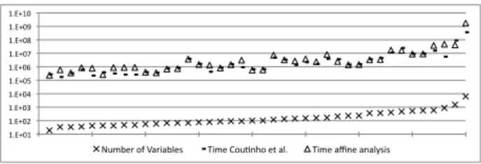
constraints took 58.6 msecs to go over all the 177 kernels. Figure 7 compares the analysis runtime with the number of variables per program, considering the 40 chosen kernels only. The top chart measures time in CPU ticks, as given by the rdtsc x86 instruction. The coefficient of determination between these two quantities, 0.972, indicates that in practice our anal-ysis is linear on the number of variables in the target program. Figure 7 also compares the runtime of our analysis with the divergent analysis originally present
!"#$%!& !"#$%'& !"#$%(& !"#$%)& !"#$%*& !"#$%+& !"#$%,& !"#$%-& !"#$%.& !"#$!%&
/01234&56&784982:3;& <913&=50>?@5&3A&8:"& <913&8B?3&8?8:C;9;&
Figure 7: Time, in CPU cycles, to run the divergent analyses compared with the number of variables per kernel in GSA-form. Points in the X-axis are kernels, sorted by the number of variables they contain. We report time of analyses only, excluding other compi-lation phases.
in the Ocelot distribution. This analysis was imple-mented after Coutinho et al.’s [2], and was available by default in Ocelot until revision 1520, when it was replaced by our algorithm. On the average, our anal-ysis is just 1.39x slower, even though Ocelot’s old analysis only marks a variable as uniform or not. Precision of the divergence analysis with affine constraints: Figure 8 compares the precision of our analysis with the precision of the old divergence anal-ysis of Ocelot. Ocelot’s analanal-ysis reports that 63.78% of the variables are divergent, while we report 58.81%. However, the old divergence analysis can only mark a variable as uniform or not [2]. On the other hand, our analysis can find that 24.84% of the divergent variables are affine functions of the thread identifier. Register allocation: Figure 9 compares three dif-ferent divergence aware register allocators. We use, as a baseline, the linear scan register allocator [16] that is publicly available in the Ocelot distribution, and is not divergence aware. All the four allocators use the same policy to assign variables to registers and to spill variables. The divergence aware alloca-tors are: (DivRA) which moves to shared memory only the variables that Ocelot’s old divergence analy-sis [2] marks as uniform. This allocator can only use the row (ii) in Figure 6; (RemRA), which does not use shared memory, but tries to eliminate stores and replace loads by rematerializations of spilled values that are affine functions of Tid with known constants. This allocator uses only rows (i) and (iii) in Figure 6; (AffRA), which uses all the four rows in Figure 6, and is enabled by this paper’s analysis.
Times are taken from the average of 15 runs of each kernel. We take about one and a half hours to execute the 40 benchmarks 15 times on our GTX 570 GPU. Linear Scan and RemRA use nine registers, 6
!" !#$" !#%" !#&" !#'" (" l s . c v t p . t n k m . i m t n . t n d 8 . q f t n . t f t n . t g t n . t b t n . t c r g . d t t p . t p b f . k l c f . c r t n . c s c f . c p t n . t d l s . c k b p . a d s m . i d m t . b m b p . l y d 8 . 1 d d 8 . 1 l k m . k p s d . s 2 b s . b s m m . m m m t . r g h t . c p s d . s 1 d 8 . 2 d d 8 . 2 l n w . n 1 n w . n 2 d 8 . l d d 8 . d c r g . d r c n . m k c f . c x h t . k l A r i t h M e a n )*+,"-./012." )*+,"3415"
Figure 8: Percentage of divergent variables reported by our divergence analysis with affine constraints and the divergence analysis of Coutinho et al. [2]. Kernels are sorted by the number of variables.
!"#$%&' !"#$%(' !"#$%)' !"#$%*' !"#$%+' !"#$!%' !"#$!!' !" !#$" !#%" !#&" !#'" (" (#$" bf. kl ht. cp d8. ld sm. id d8. 1l rg. dt d8. qf d8. dc bp. ly d8. 2l bp. ad ls. cv mm. mm ls. ck ht. kl km. im sd. s2 tn. tf tn. tg tn. cs sd. s1 d8. 1d tn. tn tn. tb tn. tc tn. td nw. n1 n2. n2 tp. tn tp. tp d8. 2d rg. dr cf. cr mt. bm cn. mk mt. rg cf. cp km. kp bs. bs cf. cx Geo Mea n )*+),-./" 012),-./" ,3),-./" !" #$" $$" #%" &%" &&!" #" %$" &'" &%" &(" !" #%" &$" )$" (" **" (" (" +"&(%" #(" *"
&" &" &" !$" '&" (" !" &&$"
&'" +" &&" &'" *" +" &" &'" )%*" &$##" ,⊥-⊥. " /012"#3",(-⊥.4" /012"*3",5-5.4" /012"!3",5-⊥.4"
Figure 9: From top to bottom: (i) Runtime of the kernels after register allocation using AffRA. (ii) Relative speedup of different register allocators. Every bar is normalized to the time given by Ocelot’s linear scan register allocator. The shorter the bar, the faster the kernel. (iii) Static number of instructions inserted to implement loads of spilled variables. Numbers count loads from local memory that have not been rewritten. SDK’s Kmeans::invert mapping (km.im) and Transpose::transpose naive did not contain spill code.
whereas DivRA and AffRA use eight, because these two allocators require one register to load the base address that each warp receives in shared memory to place spill code. Each kernel has access to 48KB of shared memory, and 16KB of cache for the local memory. On the average, all the divergence aware register allocators improve on Ocelot’s simple linear scan. The code produced by RemRA, which only does rematerialization, is 7.31% faster than the code produced by linear scan. DivRA gives a speedup of 12.75%, and AffRA gives a speedup of 29.70%. These
numbers are the geometric mean over the results in Figure 9. There are situations when both DivRA and AffRA produce code that is slower than the Ocelot’s linear scan. This fact happens because (i) the local memory has access to a 16KB cache that is as fast as shared memory; (ii) loads and stores after rewriting take three instructions each, according to rule four of Figure 6: a type conversion, a multiply-add, and the memory access itself; and (iii) DivRA and AffRA insert into the kernel some setup code to delimit the storage area that is given to each warp.
Figure 9(Bottom) shows how often AffRA uses each rewriting pattern in Figure 6, column “Load”. The tuples (0, ⊥) ↓, (c, c) ↓ and (c, ⊥) ↓ refer to lines ii, iii and iv of Figure 6, respectively. We did not find opportunities to rematerialize constants; thus, the rules in the first line of Figure 6 have not been used. (⊥, ⊥) ⇓ represents loads from local memory that have not been rewritten. Overall we have been able to replace 46.8% of all the loads from local memory with more efficient instructions. The pattern (0, ⊥) ↓ replaced 24.1% of the loads, and the pattern (c, ⊥) ↓ replaced 15.3%. The remaining 7.4% modified loads were rematerialized, i.e., they were replaced by the pattern (c, c) ↓. Stores from local memory have been replaced similarly. For the exact numbers, see [18].
6
Conclusion
This paper has presented the divergence analysis with affine constraints. We believe that this is currently the most precise description of a divergence analysis in the literature. This paper has also introduced the notion of a divergence aware register allocator. We have tested our ideas on a NVIDIA GPU, but these techniques work in any SIMD-like environment. As future work, we plan to improve the reach of our anal-ysis by augmenting it with symbolic constants. We also want to use it as an enabler of other automatic optimizations, such as Coutinho et al.’s branch fu-sion, or Carrillo et al.’s [17] branch splitting.
Reproducibility: our code is publicly available in
Ocelot, revision 1521, June/2012. All the
bench-marks used in this paper are publicly available. For more information about the experiments, see our website at http://simdopt.wordpress.com.
Extended version: a more extensive discussion
about our work, including the proof of Theorem 3.1, is available in the extended version of this paper [18].
References
[1] A. Aiken and D. Gay, “Barrier inference,” in POPL. ACM Press, 1998, pp. 342–354.
[2] B. Coutinho, D. Sampaio, F. M. Q. Pereira, and W. M. Jr., “Divergence analysis and optimizations,”
in PACT. IEEE, 2011.
[3] R. Karrenberg and S. Hack, “Whole-function vector-ization,” in CGO, 2011, pp. 141–150.
[4] J. A. Stratton, V. Grover, J. Marathe, B. Aarts, M. Murphy, Z. Hu, and W.-m. W. Hwu, “Effi-cient compilation of fine-grained SPMD-threaded
programs for multicore CPUs,” in CGO. IEEE,
2010, pp. 111–119.
[5] G. Diamos, A. Kerr, S. Yalamanchili, and N. Clark, “Ocelot, a dynamic optimization framework for bulk-synchronous applications in heterogeneous systems,” in PACT, 2010, pp. 354–364.
[6] E. Z. Zhang, Y. Jiang, Z. Guo, K. Tian, and X. Shen, “On-the-fly elimination of dynamic irregularities for
GPU computing,” in ASPLOS. ACM, 2011, pp.
369–380.
[7] P. Briggs, K. D. Cooper, and L. Torczon,
“Remate-rialization,” in PLDI. ACM, 1992, pp. 311–321.
[8] S. Che, M. Boyer, J. Meng, D. Tarjan, J. W. Sheaf-fer, S.-H. Lee, and K. Skadron, “Rodinia: A bench-mark suite for heterogeneous computing,” in IISWC. IEEE, 2009, pp. 44–54.
[9] K. J. Ottenstein, R. A. Ballance, and A. B. Mac-Cabe, “The program dependence web: a representa-tion supporting control-, data-, and demand-driven interpretation of imperative languages,” in PLDI. ACM, 1990, pp. 257–271.
[10] P. Tu and D. Padua, “Efficient building and placing of gating functions,” in PLDI. ACM, 1995, pp. 47– 55.
[11] W. W. L. Fung, I. Sham, G. Yuan, and T. M. Aamodt, “Dynamic warp formation and scheduling
for efficient GPU control flow,” in MICRO. IEEE,
2007, pp. 407–420.
[12] A. W. Appel, “SSA is functional programming,” SIGPLAN Notices, vol. 33, no. 4, pp. 17–20, 1998. [13] A. V. Aho, M. S. Lam, R. Sethi, and J. D. Ullman,
Compilers: Principles, Techniques, and Tools (2nd
Edition). Addison Wesley, 2006.
[14] F. Nielson, H. R. Nielson, and C. Hankin, Principles
of Program Analysis. Springer, 1999.
[15] S. Ryoo, C. I. Rodrigues, S. S. Baghsorkhi, S. S. Stone, D. B. Kirk, and W. mei W. Hwu, “Optimiza-tion principles and applica“Optimiza-tion performance evalua-tion of a multithreaded GPU using cuda,” in PPoPP. ACM, 2008, pp. 73–82.
[16] M. Poletto and V. Sarkar, “Linear scan register allo-cation,” TOPLAS, vol. 21, no. 5, pp. 895–913, 1999. [17] S. Carrillo, J. Siegel, and X. Li, “A control-structure splitting optimization for GPGPU,” in Computing
frontiers. ACM, 2009, pp. 147–150.
[18] D. Sampaio, R. Martins, S. Collange, and F. M. Q.
Pereira, “Divergence analysis with affine
con-straints,” ´Ecole normale sup´erieure de Lyon, Tech.
Rep., 2011.