Child contribution to agricultural household income

DAVID-ALEXANDRE BRASSARD

CHILD CONTRIBUTION TO AGRICULTURAL

HOUSEHOLD INCOME

Mémoire présenté

à la Faculté des études supérieures et postdoctorales de l'Université Laval

dans le cadre du programme de maîtrise en économique

pour l'obtention du grade de Maître es arts (M.A.)

DEPARTEMENT D'ECONOMIQUE

FACULTÉ DES SCIENCES SOCIALES

UNIVERSITÉ LAVAL

QUÉBEC

2012

R é s u m é

Le travail des enfants est un sujet qui gagne en importance en économie du développement. Les travaux se concentrent principalement sur les causes sous-jacentes du travail des enfants et les interrelations entre le travail des enfants et les décisions parentales. Rares sont les papiers qui essaient d'estimer la contribution des enfants dans le revenu familial. Cela peut être lié au fait que les enfants travaillent généralement à l'extérieur du marché du travail et cela complique grandement l'estimation de la valeur de leur travail. En fait, la majorité des enfants oeuvrent dans l'entreprise agricole familiale et ne reçoivent aucun salaire pour leurs efforts. Notre approche se base sur cette particularité du travail des enfants et la contribution du travail des enfants dans le revenu familial, sera estimée à travers l'élasticité de la fonction de production par rapport au travail des enfants. En util-isant une fonction de production, l'endogénéité des inputs sera traité avec un modèle de première différence. Les données ougandaises divisent la pro-duction agricole annuelle en deux saisons et cette division des données per-met l'élimination des effets fixes du ménage sur la production agricole. Les ménages qui produisent pendant deux saisons consécutives sont utilisés pour obtenir des estimés rigoureux de la contribution des enfants au revenu fa-milial. Le choix de l'Uganda est justifiable par l'importance du travail des enfants et par le fait que les enfants sont presque uniquement employés en milieu agricole.

Abstract

Child labor is an issue of growing importance in development economics. The focus is centered on the underlying causes of child labor and the rela-tionships between child labor and household decisions. Few papers attempt to capture children's contribution to families' income. The near absence of child labor markets complicates the estimation of child labor value. In fact, most child laborers are involved in self-employed agriculture and our ap-proach will rely on this feature to estimate children's contribution through the labor elasticity of household agricultural production. With a production function approach, we will treat endogeneity using a first-difference model, which utilizes the division of data between two cropping seasons in an Ugan-dan dataset. We use data on two cropping seasons to eliminate household fixed effects from our production functions thus, obtaining consistent esti-mates of children's contribution to household agriculture. Using the labor elasticity of household production, we evaluate the value of children's time and the obtained estimates will serve in the calculation of their overall con-tribution to household income, including agricultural and domestic labor. Uganda, with a high prevalence of child labor and the importance of the agricultural sector, is a ideal country to study child labor and the impact of children in household income.

Remerciements

J'aimerais d'abord et avant tout remercier ma directrice de thèse, Habiba Djeb-bari, qui m'a aidée et épaulée dans le processus complet entourant l'écriture du mémoire. Ses commentaires entrêmement pertinents et son sens critique très développé m'ont grandement aidés dans la rédaction de ce travail, et plus par-ticulièrement dans ma compréhension de la rigueur nécessaire dans l'étude de la science économique. De plus, j'aimerais la remercier de sa grande tolérance et compréhension face à mon approche relativement non orthodoxe dans l'avancement de mon mémoire. En résumé, ce fut très instructif et amusant d'apprendre de vous, Mme Djebbari.

Il est aussi très important de mentionner l'apport de mon codirecteur Monsieur John Cockburn, qui avec sa connaissance approfondie du sujet et sa compréhension globable du travail des enfants, a permis d'éclairer et de grandement faciliter mon apprentissage. Il est également primordial de mentionner que ce mémoire porte sur un sujet que John Cockburn avait profondément exploré dans ces études doctorales et sa thèse fut l'inspiration de ce mémoire. J'aimerais aussi remercier John puisqu'il m'a permis à travers ses multiples contacts de travailler sur mon mémoire dans les bureaux d'UXICEF en Uganda et cette expérience a été très enrichissante.

Pour finir, j'aimerais également remercier Sylvain Dessy pour son apport en tant que correcteur mais aussi pour son rôle de directeur du deuxième cycle à travers duquel il m'a permis d'accéder à deux directeurs de maîtrise géniaux. De plus, il a grandement aider dans la compréhension du processus scientifique en-tourant l'écriture et la présentation d'un mémoire.

Contents

1 Introduction 1 2 Literature review 3

2.1 On child labor 3 2.2 Public policy 6 2.3 Agricultural shadow wage 8

3 Child labor in an agricultural household model 11

4 Econometric Model 18 5 D a t a 21 5.1 Sampling restrictions 23 5.2 Sample characteristics 23 6 Empirical Application 28 6.1 Functional form 29 6.2 Labor elasticity of agricultural production 31

6.3 Cross-sectional estimation 33 6.4 First-difference Model 40 7 Conclusion 45 8 References 47 8 Appendix 50 IV

List of Tables

1 Production characteristics 25 2 Cross-sectional estimation 35 3 Translog interaction terms 36

4 GCD estimation 37 5 Labor elasticities of household production in agriculture 38

6 Shadow wages in cross-sectional analysis 38

7 First-difference regressions 42 8 Shadow wage with first-difference model 43

9 First-stage regressions 52

List of Figures

1 Self-reported labor participation 22 2 Average time spent in agricultural activities (2004) 26

3 Age patterns in domestic work per week 28 4 Gender disparities in domestic work per week 29 5 Children work time for sectors and regions 45

1 Introduction

The purpose of this study is to estimate the contribution of children in household income. Their contribution is rarely well captured and this paper will try to fill this gap by offering robust labor elasticity estimates in order to estimate children shadow wages. Furthermore, the estimates obtained in this research can be used to evaluate the value of domestic work since children simultaneously involved in domestic and agricultural tasks should have identical shadow wages in both activ-ities.1 Assigning a value to children's time provides quantitative information for

the design of public policies to adress the issues of child labor. In fact, the esti-mates could be used to determine the value of conditional cash transfer, necessary to promote schooling in Uganda.

The prevalence of child labor is especially high in low-income countries and as such, sub-Saharan Africa has the highest incidence of child labor, where almost a third of all children are involved in economic activities. The focus on sub-Saharan Africa is therefore understandable. This paper will use data from the National Household Survey of Uganda (NHSU). This choice is far from arbitrary as 38, 2% of children in Uganda are involved in economic activities, exceeding the sub-Saharan trend in child labor incidence. In addition, 95, 5% of Ugandan child workers are in the agricultural sector thereby defending our approach to use agricultural production as a proxy for the value of child labor.2

Economic literature has taken steps towards a better understanding of the phenomenon of child labor. Most papers are generally centered around the parental decision to divide children's time between leisure, schooling and work. The relative value of each opportunity is weighted by the parents. For example, a parent can

'The model presented in section 3 explains extensively this relationship between the shadow wages of agricultural labor and domestic work.

choose to send his child to work if there are no government public schools in their village. On the other hand, the presence of a school might not affect the parental decision to send his child to work, if the amount of agricultural work that can be accomplished by the children is central to household income. Parental decision will be guided by the contribution of children in household income and their impact on agricultural production is therefore important in the choices regarding children time allocation.

The evaluation of children's contribution to household income has been adressed in a few papers. However, the economic literature focuses on the determinants of child labor, policy implications and the link between child labor and household decisions. The datasets of developing countries are relatively restrictive in terms of precise child time allocation data and it could explain the literature's focus. In addition, the characteristics of child labor complicate the estimation of children's contribution to income. Most child workers are employed inside the household and child labor markets are by consequence almost inexistent. Furthermore, children rarely receive compensations for their work and the direct link between the value of work and wages is eradicated.

Pioneer papers by Jacoby (1993) and Skoufias (1994) estimate the value of work outside of labor markets, which is named shadow wage. They use household level production functions and estimate the value of agricultural work using the marginal productivity of household members. The authors focus on adult labor, as most empirical studies on the estimation of agricultural shadow wages do. Our methodology is based on Cockburn (2001), in which the author adressed the con-tribution of children in household income with a production function approach. The author includes domestic labor in his estimations of children's contribution to household income.

The difficulty in properly assessing children's contribution is also linked to the fact that input choices in an household production function are endogenous. In the literature, instrumental variables is the preferred method to treat endogeneity but in developing country datasets, valid and relevant instruments are scarce. In our model, agricultural production is expressed within an annual framework divided in two cropping seasons. This panel feature of the dataset can be used to estimate the contribution of children with a first-difference model since most households produce in both cropping seasons. The first-difference model should eliminate household fixed effects and offer consistent estimates of children's impact on agricultural production through the labor elasticity of household production.

A summary review of child labor literature is presented in section 2. In section 3, an agricultural household model is presented to explain parental decision regard-ing child labor. The first-difference model is presented in section 4 and section 5 contains a discussion on the dataset. The empirical application of our model is presented in section 6.

2 Literature review

2.1 On child labor

According to the International Labor Organization (ILO), 300 million children are working in the formal and informal sector worldwide in 2010. Those estimates include children from 5 — 17 involved in economic activities and exclude children involved in domestic work. That number can be compared to the global population of children estimated at 1.586 billion. The importance of children in economies is global and the interest of this research surrounds the concept of child labor. The term child labor is often used to describe children involved in economic activities. In this paper, child labor will be defined as children under 12 who are involved

in economic activities whether it is market work or self-employed labor, children under 15 who are involved in 14 hours of work per week or at least 1 hour of hazardous work and children between 15 and 17 involved in worst forms of child labor such as forced labor, armed conflict, prostitution, pornography or illicit activities. The definition of child labor used in this research emerges from the ILO, which also set the minimum working age at 15.3

The objective of this research is to determine the value of child work in self-employed agriculture. The focus will be on children under the age of 15 therefore, children work included in the analysis is not necessarily child labor as children between the age of 12 and 14 are not always meeting the criteria of 14 hours of self-employed labor. At first glance, this could seem problematic as some children included in the analysis are not involved in child labor. But, since the main purpose of this research is to determine the average value of children's time in agriculture, the estimated average can be used equally to describe child laborers or child workers.

Child labor has been studied through the impact it can have on household decisions. Rosenzweig and Evenson (1977) introduce a household model to study the tradeoff between children's schooling and work in parental decisions. The main findings of this paper surrounds the impact of that tradeoff in fertility decisions. They find that the large number of children in Indians families, in the late 1950s, is motivated by the higher return of children's work in comparison to schooling opportunities. Following their methodology, Levy (1985) finds a link between large family sizes and proxies for high economic contribution of children in Egyptian data. The fertility decisions of parents is also studied in Cain (1977), who concludes that high fertility rates in Bengladesh is rational because of the importance of children in household income. However, later empirical works have questionned

internationally-the link between child labor and fertility with accounting approaches, notably Lee et al. (1983) and Stecklov (1999).4 The difficulty in properly assessing the

impact of child labor on fertility justifies the need for robust children shadow wage estimates.

Additionally, increasing hours of child labor can have a impact on time spent at school or doing homeworks. This relation has been studied in empirical works focusing on comparative statistics. For example. Psacharopoulos (1997) finds that child laborers complete two school years less than their non-working counterparts. They also noted that the probability of grade repetition was associated with child labor in Latin America. In a Tanzanian dataset, Akabayashi et al. (1999) find that factors affecting positively school time have a negative impact on working time, indicating the presence of a tradeoff mechanism. Ravallion and Wodon (2000) specifically approach the identification of a causal link between education and labor in Bangladesh. They study the impact of an exogenous shock on the price of schooling created by subsidies for education. The reduction in school prices is followed by an increase in enrollment rates. This time use trend is mostly created by a reduction of leisure time. Nonetheless, the subsidies reduce the working time of children and they conclude that the relative value of child work, in comparison to the costs of education, has an impact on schooling time.

Child labor can also have an impact on child health by placing children in environments prone to injuries and physical hazards. The health risks can be more subtle and present themselves long after children's entrance in economic activities. For example, a children working in an environment filled with dust and dirt can develop lung problems after repeated exposure. Graitcer and Lerer (1998) compare morbidity, injuries and hazards between different work environments for children

4 Both papers sum expenses related to children and compare the obtained aggregates to the

and conclude that even self-employed agriculture could be risky for children. Apart from the possible effects child labor can have on fertility, schooling and health, child labor can form an subsantial part of household income. Few papers try to directly estimate the value of child work. Among those, Cain (1977) notes that children in a village of Bengladesh become net producers by the age of 12 and account for their whole life consumption when they reach fifteen years of age. Evenson et al. (1980) estimated that children contribute for a quarter of their household's total income. Including home production in their analysis, the contribution of all children are almost three quarters of the father's contribution in rural Philippines. Cockburn (2001) estimates the contribution of a single child to be roughly 4 to 7 % of household income using Ethiopian data. Along those lines, Menon et al. (2005) have estimated the value of children agricultural shadow wages to be close to 60% of the adult's. Extrapolating their estimates to the entire Nepalese economy, the authors have determined that children could account for 9% of the country's gross domestic product. The authors mentionned above all show that child labor is undeniably important in terms of income and the impact it can have on household behavior.

2.2 Public policy

Historically, policy-makers have adressed child labor with human rights' consider-ations. The morality question associated with child labor in high-income countries has emerged following the importance of child work in the Industrial Revolution. Regulations on child labor in Western societies have followed England's Factory Acts with stricty imposed legal working age, trying to ban child labor. This ap-proach is symbolized by the United States' Child Labor Deterrence Act of 1997, which seeks to ban the import of goods produced with child labor inputs. Those drastic measures may be considered as a method to get rid of child labor.

How-ever, banning child labor is not necessarily welfare improving if households and national economies crucially depend on the income generated by children. Fur-thermore, those laws are hard to implement as they require government control and surveillance over labor markets.

On the subject of policy evaluation, Basu and Van (1998) present an interest-ing theorical model. The model makes two different hypotheses concerninterest-ing the underlying causes of child labor. First, the luxury axiom stipulates that a parent will send his child to work if the household's income without child labor is very low. Second, the substitution axiom assumes that adult labor can be substituted by child labor. These hypotheses have a realistic edge and the authors present an economic model with a possibility of multiple equilibria. In other words, an econ-omy can have children working and not working while both situations are part of an equilibrium behavior. The authors' model is used to evaluate the impact of a potential ban of child labor on household welfare. The results of the ban will depend on the initial single or multiple equilibria of the economy. Basu and Van (1998) therefore show that systematically treating child labor with regulations and strict bans could be a approach that needs to be revisited. The authors have managed to put some perspective in the policy treatment of child labor.

Recently, alternative policies have emerged to deal with child labor and those policies aim at altering household incentives. For example, subsidies for education reduce the price of schooling for households and can affect the decision of a parent to send his child to work. Cash transfers conditional on education can have the same effect on child labor by modifying the relative returns of schooling. Theses program are gaining in popularity as policy-makers around the world are treating child labor and different poverty issues with conditional cash transfers (CCT).5

In the list of countries figures Mexico, Brazil, Colombia, Honduras, Bangladesh, Namibia, Zambia, Kenya, Lesotho, Tanzania and Mozambique.

Skoufias (2001) presents results indicating a positive impact on schooling time and a negative impact on child labor time associated with the introduction of a CCT program in Mexico. Ravallion and Wodon (2000) find similar results related to subsidies on education in Bangladesh. The theoretical and empirical papers presented in this section indicate that alternative policies should be used to deal with issues linked to child labor. The efficiency of altering household incentives will depend on the importance of children in household income. In a policy-making context, the evaluation of children shadow wages can determine the needed modifications in household incentives. The evaluation of children shadow wages is consequently central to policy-making.

2.3 Agricultural shadow wage

The economic literature on shadow wages takes two different routes in empirical es-timation. First, the primal side estimation relies on the derivation of a production function to obtain marginal productivities. Second, the dual side uses cost and profit functions to estimate the value of agricultural work. Deriving the shadow wages in the dual approach requires the hypothesis that child labor inputs have a quasi-fixed nature.6

The idea of estimating the marginal product of labor in agriculture using a pri-mal side framework applied to developing economies has been introduced by Rosen-zweig (1980). The author presents an application of the neoclassical approach in the determination of household labor supply in rural India. The household model presented is a two-step maximization of household welfare, in which the house-hold first maximizes the farm profit and then maximizes the utility conditionnai on the farm's profit. Therefore, the "recursive" model assumes a separability

be-6Cost and profit functions use the price of variable inputs and the quantity of fixed inputs

in their formulations. Thus, in order to derive the value of child labor, this input has to be considered quasi-fixed.

tween the production and consumption decisions of households. This separation in household's decisions relies on the assumption that a household will maximize his profits treating hired and self-employed labor as perfect substitutes. Under this assumption, the value of family labor is simply equal to the average market wage.7 This hypothesis seems problematic when applied to a sub-Saharan economy, where landless agricultural workers are relatively rare in rural areas. Furthermore, the hypothesis of substituability relies on the presence of perfectly functioning labor markets and a mobile labor force. The author's purpose is the estimation of house-hold labor supply and the value of shadow wage is estimated with the market wage. The imputation of a market wage to agricultural labor, using average community wages from household surveys, neglects the particularities of self-employed labor and requires extremely reliable community data on wages.8

Heckman (1974) presented a method to estimate the shadow wage of married women taking into account their relatively low participation in market labor. He incorporates the factors affecting the decision to work for market wages in an equation to estimate shadow wages. His approach is interesting in a context with sufficient data on market laborers but for the particular case of children in a developing country, Heckman's approach is hard to implement.

The seminal paper of Jacoby (1993) presents estimates of agricultural shadow wages in Peru without relying on a theoretical "recursive" model. The shadow wage estimates are obtained by deriving the marginal product of labor using a household level production function. The shadow wages are assumed to differ from the market wage because the production and consumption decisions are no longer separable. In addition, the author uses estimated shadow wages in the

7This conclusion relies on the absence of unemployment and transaction cost associated with

market labor.

Community wages are generally collected with questionnaires delivered to community leaders and the declared wages will depend on the ability of this economic agent to evaluate the market wage.

determination of a labor supply function for male and female adult workers. Skoufias (1994) presents a paper that derives shadow wages from a production function with a household model similar to Jacoby (1993). The author treats endogeneity using panel data on rural Indian villages and isolates household fixed effects. However, Skoufias (1994) focused on adult labor and the shadow wages were simply intermediate estimates in the determination of adult's labor supply functions.

In the shadow wage literature, Barrett et al. (2008) have estimated agricultural shadow wages with a primal side approach. Focusing on Ivorian rice producers, they allow the marginal value of labor to differ from the shadow wages. Their method relies on the possibility of an allocation inefficiency in household behavior. They utilize workers employed simultaneously in wage market and self-employed tasks. In a utility maximization framework, workers should only work simultane-ously on both tasks if the marginal product of agricultural labor is equal to the market wage. They notice systematic deviation from this maximisation rule that the author associate to allocative ineffiency. The shadow wages are estimated by combining this inefficiency to the marginal product of labor. The estimation of allocative inefficiency for workers not employed in both tasks are predicted with the sample of workers employed in both sector. The weakness of this methodol-ogy relies on the fact that self-employed agricultural workers are rarely involved in labor markets and this is especially true for children. This method would by consequence be inadequate for our analysis.

Dual side estimation is presented for African economies in Adesina et al. (1996) and Jayne et al. (1994). Both papers present a profit function and derive the shadow value of agricultural labor. Profit functions use prices of outputs and inputs as variables and the exogenous nature of these variables explains the interest for dual side estimates.

The formulation of a profit function differs from a production function in the sense that outputs can hardly be treated as a single aggregate because outputs are expressed in prices instead of quantities. The agriculture in Uganda is centered on six outputs produced in relatively similar proportions. The elaboration of a profit function would require a multi-output profit function with a system of output supplies and input demands. Interestingly, Menon et al. (2005) use a multi-output cost function approach to the determination of children shadow wages. They treat for censored outputs using a Heckman two-step estimator. The categories of outputs used are aggregates and the division between crops seems arbitrary. The endogenous nature of labor inputs is also not addressed in the paper.

Recently, Le (2009) presents a method to calculate shadow wages without es-timating a production or a dual side function. The maximization properties of an agricultural household model allow the simultaneous estimation of shadow wages, shadow income and labor supply functions.9

In light of the empirical literature presented, the choice of a evaluation method-ology can be directed towards different methodologies and a consensus on the right method has not been reached. The choice of a method will generally be guided by the production process of the region studied and the particularities of the available datasets.

3 Child labor in an agricultural household model

Families in the rural sector of developing countries are often simultaneously pro-ducers and consumers in the agricultural market. The economic literature has developed household modelling to address this issue. The main assumption of

9The procedure requires an intermediate input that is widely used and whose price is

deter-mined by a competitive market. In a Vietnamese sample, fertilizers are used by most agricultural households and the fertilizer market is considered to be competitive with the presence of many private companies.

these models is that parents maximize a household utility function and decide the allocation of their children's time until they reach maturity. The model focuses on the agricultural sector since most of the child labor in Uganda is done within this sector and the modelling approach is standard in the agricultural economic literature (see Stauss et al. 1986). The household utility function has the following form :

u = u(c,e

,e

) (i)

C is the consumption of the household and £ are off-work time meanwhile the subscrict a and c stand for adults and children respectively. The inclusion of £c in

the utility function means that parents value the time their children spend off-work. This formulation is not very restrictive because the degree of parental concern can differ across households. Consumption C include agricultural commodities produced inside the household or goods bought at the market price, both products are substitutes by assumption.

The work possibilities of household members are self-employed agricultural labor in the household L j , wage employment outside the household Lj . Thereby, time (T) is spent according to the following constraint :

Tj = Lf + LJ + £J (2)

where j = (a, c)

The off-work time (£) does not differentiate between schooling and leisure time. The alternative when studying child labor is to increase time spent in education. Therefore, £ may be considered as time spent earning additionnai human capital. The agricultural production of the household (Q) is represented by F(L;K, \ ) . The agricultural labor L either comes from self-employed (LF) or hired labor (H)

: Lj—Lf + Hj. Both types of labor are assumed to be perfect substitutes. Fixed input variable (K) contains land and productive assets endowments. Household

characteristics (\) are included to reflect the ability of a household head to manage his agricultural production, which could presumably affect outputs. The household budget constraint will take the following form :

pC < pF(La : Lc; K,X) - wa(Ha - Lwa) - wc(Hc - L") + Y (3)

where wt is the market wage and Y is non-labor income. Price p will be normalised

without loss of generality in the model.

This model is "recursive" since the household can first maximise farm profits and include optimized profits in the income constraint for the maximization of consumption, thus separating production and consumption decisions. This type of approach is allowed because the optimal conditions of a joint utility maximization are similiar to the first order conditions of separated maximization. The first order conditions on the production side, when maximised subject to total labor and production constraints are :

dF

dLf

dF M

= Wj , j = a,c (5)

dH

From (4) and (5), the household will use hired labor or self-employed labor by comparing their respective marginal productivity to the market wage. The household will hire in workers if their marginal productivity is equal or greater than the market wage and a similar reasoning apply to self-employed work. If the marginal productivity of both types of work is equal to the market wage, households are indifferent between self-employed and hired labor. In this case, children shadow wages could be estimated with the market wage of children as was done for adults in Rosenzweig (1980).

Recursive models rely on the hypothesis that all goods are tradable and la-bor markets are perfectly functioning. Those assumptions seem more realistic

in high-income countries as labor markets are developed and virtually all goods are tradable. However, subsistence farming is an important component in the economies of developing countries and well functioning labor markets are strongly questionned in the literature (see Deolalikar and Vijverberg 1987). Gronau (1977) includes non-tradable production (Z) in household modelling to study the impact of women's domestic work in the United States. The commodity Z is produced and consumed by the household and is not subject to market transactions or pric-ing. The household production function of domestic goods has the following form

Z = Z ( Dc, Da;x) (6)

where Dc and Da are time spent in domestic work by household members. The

modelling has typically treated Z as a good resulting from domestic production but the only requirement for the non-recursive model to apply is the absence of a transaction possibility for good Z. In a setting where output markets are almost totally absent, Z could be a type of agricultural output produced and consumed by the household. The home produced commodity (Z) created is included in the total value of consumption : C = Z + PXM, where XM will be a commodity that is either produced by the household or bought on the market.10

Furthermore, self-employed labor L? and hired labor Hj are no longer treated as perfect substitutes in the production function Q = F(L?, Hj\K,X) leading to

''XM is tradable on output markets and difierenriate from Z with this characteristic.

the new maximization problem : max U(Xm + Z , £a, Q (7) Lf,LJ,Hj,Xm,Z,Dj subject to Tj = Lf + LJ + lj + D, (8) Z = Z(Dc,Da;X) (9) pXm < p F ( LF a, LF, Ha, Hc- K ,X) - w]( Hj- L J ) + Y (10) LJ > 0 (11)

The introduction of LJ comes from a non-negativity constraint associated with the assumption that children and adults can be employed in wage employment outside the household. The price p is normalized and is similar for market and agricultural home produced goods.

Maximizing the farm profit with a recursive approach will lead to the same first order conditions expressed in (4) and (5). However, the joint maximization of the household utility in regards to production and consumption decisions will lead to different first order condtions. This feature renders impossible the separate maximization of production and consumption decisions. The joint maximization of the household utility is easily obtained by inserting the time (8) and home production (9) constraints into the objective function as seen in Skoufias (1994). The maximization problem of the household utility function leads to the following

first order conditions : dU dLF dU dLJ dU ~dD3 dF

x

Conditions (12), (13), (14) demonstrate the reduction of leisure associated to an increase in working time. The marginal impact of LF, LJ and Dj on leisure are

identical. Therefore, the left side of equations (12), (13), (14) reflect the shadow value of children's leisure and the value of agricultural work is equals to :

s^-«* + ?-«* m

The lagrange multiplier A is associated with the consumption constraint (10), meanwhile Uj is linked to the non-negativity constraint (11). The multiplier A is the marginal impact of an increase in consumption on household utility, at the maximized utility level. In other words, the value of increasing consumption without increasing income or revenues. The interpretation of \ij is more complex as the lagrange multiplier is associated with a non-negativity constraint.11 pj

measures the marginal impact of relaxing the non-negativity constraint meaning that household could work negative hours in wage employment, which at first glance makes no sense. However, the multiplier can be understood properly by linking it to the time constraint (8) because it measures the impact on household utility of increasing LF,£j,Dj without increasing T. The coefficient ^ in (16)

applied to children can be visualized as the impact of increasing leisure time (£)

nT h e analysis is much simpler when the constraint is not binding. However, many households

do not participate in wage employment in sub-Saharan Africa.

divided by the impact of increasing consumption. Therefore, the value of child work (u;*) depends on the tradeoff between child leisure time and consumption in household utility functions.

The shadow wage of self-employed work in the presence of possible failures in the labor market, differs from the market wage. This distinction applies to self-employed workers who are only economically involved inside the household. As presented in (15), hired labor will be used in household production up to the point where the marginal productivity of hired workers is equal to the market wage. Following this logic, a person simultaneously involved in wage employment and self-employed tasks needs to have a shadow wage that is equal to the market wage. This conclusion comes from the utility maximization requirements and the term p. would equal zero for those workers as the constraint is binding. Equally, children involved in simultaneous domestic and agricultural work have an identical shadow wage for both activities. Hence, the non-recursive household model allows the estimation of children's contribution to household income through agricultural work and domestic tasks, which together corresponds to most of children's income-generating activities.

Children are rarely involved in self-employment and wage employment simulta-neously therefore strengthening the need to estimate the shadow wage for children with (16). Interestingly, empirical works by Jacoby (1993), Skoufias (1994) and Le (2009) have all rejected the hypothesis of equality between market wages and the shadow wages of self-employed agricultural workers.

This approach to household modelling justifies the derivation of production function to obtain shadow wages estimates. However, the model's only purpose is to explain the use of production in the determination of children's shadow wages. There is no new information included and the contribution of this paper relies on the first-difference model.

4 Econometric Model

Agricultural production in Uganda is divided between agricultural seasons and we utilize this characteristic to model production using a panel approach. Household production can be expressed with the following equation :

Yit = a, + X'u k t3k + LFcltBx + St + eit (17)

where household i produces at season t. The panel approach is applied in a annual framework which contains two different agricultural seasons. Therefore, t takes the value of 1 or 2 in the estimation.

The matrix Xitk includes A; production inputs except child labor which is

ex-pressed by LF t. Household fixed effects are expressed by ai and seasonal fixed

effects are captured by 5t. Parameter a, is time invariant and that assumption is

weakly restrictive because the time variables are seasons thus leaving relatively less time for changes in household behavior and characteristics. We assume that the error terms ta are exogenous, insuring that E[tit\Xitk, LFt] — 0. This assumption

relies on the presence of household fixed effects ati which capture the household's unobservables characteristics that are correlated with Xitk and LF t. Therefore,

the inclusion of a^ in the model allows the extraction of endogeneity between the error term and production inputs.

The slope coefficient /?* and B\ are assumed to be identical in both seasons meaning that labor is equally productive throughout the year when household and seasonal fixed effects are included in the model. With productive inputs such as land cultivated or material inputs this assumption seems to hold because those inputs would likely have a similar impact on household production in both seasons. However, this hypothesis would be incorrect in a context where household labor force systematically works loss efficiently during one of the cropping season. This difference in marginal productivity of labor could be linked to holidays or simply

seasonal work habits. The assumption on the absence of seasonality could be incorrect for market labor as wages could vary between seasons.

Household fixed effects Qi are eliminated to obtain consistent estimates of dk and Bx by subtracting the production function for the first agricultural season

from the second season, generating the following first-difference model :

Yi2 - Yn = (Xl2k - Xilk)'j3k + (LF2 - LF1)Bl + (52 - 6,) + tl2 - eiX

which can be written as

AYi = AX'ikf3k + AL^B1-r6 + Aei (18)

The model can be consistently estimated on the following assumption :

E[ti2 - t a \ Xa - XiX,L^2 - Z&] = 0 (19)

The differential error term (ei2 — (-n) is not necessarily indépendant and

identi-cally distributed because the errors (tit) could be correlated over time (Cov[t;i, ti2] ^

0) and the estimation of the model would require robust standards errors treating this serial correlation.

The model (18) can only identify the parameter 3k and B\ when the production

inputs vary between seasons, restricting the choice of inputs included in Xitk and

the sample to households with variation in child labor inputs. As expressed earlier, some households may employ children in their agricultural production but a signif-icant percentage will have no children involved in agriculture during the year and this complicates the identification of Bx. The selected sample of households with

positive values of child labor inputs could differ systematically from households not employing children during both agricultural seasons and assumption (19) would no longer hold. The choice of sending a child to work can be linked to the household head's motivation toward his agricultural heritage, where the parents want their

child to work in order to prepare for future inheritance of the household's land. This unobservable characteristic presented as motivation can positively alter the agricultural production of the household and the parameter Bx would capture this

particularity and overestimate the impact of children in agricultural production. However, the first-difference model (18) eliminates the selection issues linked to Oj and the possible selection problems need to be generated by a correlation of Ae^ with the choice of child labor inputs LFt.

The unobscrvables Ae^ could simultaneously affect child labor participation and household agricultural production through community variables such as access to institutions. For example, household with seasonal credit constraints could use child labor inputs in one of the agricultural seasons and parameter B\ would cap-ture the effects of a credit constraint on agricultural production and underestimate the impact of child work. The seasonal credit constraint has to be non-uniformly distributed in Uganda because if the whole sample has a similar difference in seasonal credit access, the impact of this constraint on agricultural production would be captured by 6. This reasoning could be applied to community access to instutions such as input and output markets, agricultural extension centers or educationnal facilities. In rural communities, access to institutions should be lower in comparison to their urban counterparts. The presence of a systematic seasonal variation between different rural communities seems unrealistic because access to market institutions and educational facilities should have little variation between the two agricultural seasons. Furthermore, if there is variation, it should be sim-ilar in other rural communities of Uganda. For example, a higher production in the second season could lead to a more developed market structure which should extend on most of the rural communities. In urban regions, access to institution should be relatively similar between seasons, accentuating the improbability of selection problems in the restricted sample of households with child laborers. For

the mentioned reasons, the panel approach should be efficient in limiting selection problems and endogeneity issues in the Ugandan dataset.

5 Data

The empirical estimation of children shadow wages uses the Ugandan National household survey (UNHS) of 2005-2006. The survey collected information on close to 7400 representative households with multiple questionnaires capturing house-hold characteristics, agricultural practices and community data.

The information was collected over a period of 12 months, in which inter-viewers made two visits to every household. The agricultural questionnaire was administered on both visits to collect information on the prior cropping season, meanwhile household and community questionnaires were only completed during one of the two visits. Hence, some variables do not vary between seasons and are consequently excluded from the first-difference model

The household questionnaire contains self-reported labor activity of household members in the week before the interview took place. Those statistics can illustrate the characteristics of labor markets in Uganda. Figure 1 represents the involvement of children and adults in economic activities excluding domestic labor from the whole UNHS sample.

The majority of active children are self-employed agricultural workers and chil-dren are not significally involved in wage employment. Furthermore, chilchil-dren are rarely involved in simulataneous economics activities such as wage employment and self-employed labor. Adults on the other side are relatively more involved in wage employment and are more prone to simultaneous self-employed and market labor. The agricultural sector represents 50% of wage employment labor, highlighting the importance of agriculture in the Ugandan sample.

Figure 1: Self­reported labor participation

100%

Children

■ Simultaneous Economic activities

D Net economics lly actK«

O Wages Employment ■ Self-Employed Other

E Self-Emptoyed Agriculture

These features of Ugandan labor markets suggest that estimating child labor with agricultural production should prove adequate, implying that shadow wage estimates could systematically differ from market wage and justify our methodol­ ogy.

The agricultural questionnaire was only given out to households who reported cultivating crops or raising livestock. Agricultural data are collected on the second cropping season of 2004 (July to December) and on the first cropping season of 2005 (January to June).12 The labor inputs in the agricultural questionnaire are

aggregates of person—days measures of male, female and child work. The labor cannot be linked to the particular child who performed it. Thus, age or gender patterns of agricultural child labor cannot be disguished among the dataset. The children category in the questionnaire includes household members under 15. The time allocation data on labor inputs refer to activities related to crop production. Therefore, households included in the sample of interest have a positive value for crop production and household only producing livestock are excluded. This

The distinction between both agricultural periods is linked with the presence of two rainy seasons.

construction is not very restrive since only 5 to 10% of agricultural producers do not harvest any crop.

5.1 S a m p l i n g r e s t r i c t i o n s

The sample includes households reporting positive crop production in both sea-sons and who employ children once during the year. Initially, 7400 representative households are reported in the UNHS of which 4658 are crop producers in both agricultural season and among those more than half, 2708 households, use child labor inputs during the year.

5.2 S a m p l e c h a r a c t e r i s t i c s

The agricultural questionnaires offer plot-level labor inputs but the agricultural crop production is presented by crop type and does not differentiate the production per plot. The amount of hours worked per type of crop can hardly be extrapolated because each type of crop might require different labor time. Thus, the agricultural production function will be expressed at the household level where labor inputs of household members are summed on all the plots. The production characteristics of the Uganda National Household survey of 2005-2006 are presented in Table 1. Crop production is the total value of crop using self-reported prices at the household level.13 The aggregation of production in value can be problematic if

there is regional variation in output prices, but we have to resort to aggregation because of the lack of other possibilities. Productive assets and material inputs are also summed at the household level to obtain the total value of each input.

The different production characteristics are presented in Table 1. The produc-tion process in Uganda is centered on labor inputs and land, as the total value of

13Extreme values reported are replaced by median prices computed at the community level.

reported productive assets and material inputs are on average under 25 000 Ugan-dan schillings (UGX) which is equivalent to 14 US$.14 In fact, the use of manure,

fertilisers or pesticides is not common in the sample.

Combining both seasons, households have an average of 3 hours of agricultural adult labor per day, which is relatively small if a household generally contains at least two adults. Time spent working on household land could be constrained by domestic work, which is equal to an average of 15 hours per week for every adult.15

Labor time could also be constrained by the absence of agricultural taks to ac-complish as the agricultural process in rural regions does not include intermediate inputs and lacks irrigation systems. This could potentielly explain the relatively low amount of time worked on household plots.

The application of the first-difference model requires variation in the production inputs between agricultural seasons. This time variation in inputs is named within-variation, meanwhile, the between variation reflects the variation in inputs between different households in the same agricultural season. As observed in Table 1, most variables tend to have a larger between-variation. This is especially true for productive assets and land area cultivated whose within-variation is relatively small. This particularity follows economic logic since those inputs are considered fixed inputs, when studied in a short time span. Identification will therefore be harder for inputs that have a tendancy to vary less across time. Furthermore, if small within-variation is combined with a minor impact on production, the identification process will be much harder.

All variables extracted from the household questionnaires have no within-variation as the questionnaire was only administered during one of the seasons.

1 4The exchange rate of 2006 was around 1800 UGX for 1 US $. Considering the purchasing

power parity conversion (PPP) rate of 0.3 in 2005 according to the world bank, 540 UGX is equivalent to 1 US dollar in purchasing power.

15This average is mainly driven up by female, who work on domestic task for close to 25 hours

a week on average.

Table 1: Production characteristics

Number of Households 2701

Number of Periods 2

Observations 5402

Mean Std. Dev. Between Var. Within Var. Variables

Crop Production (UGX) 487 672 3 944 159 2 802 374 2 775 705 Adult Labor (Hours/season) 547.2 591.7 532.3 258.5 Child Work (Hours/season) 103.5 204.9 182.09 93.9 Outside Labor (Hours/season) 110.1 494.5 382.9 312.9

Land Area (Acres) 5.9 59 59 0.88

Productive Assets (UGX) 22 077 41 507 39 923 11 370 Material Inputs (UGX) 18 423 62 548 53 395 32 585 Production Dummy Variables

Manure .07 .26 .19 .18

Pesticides .06 .24 .17 .17

Improved Seed .29 .45 .45 (I

Good Soil .40 .44 .44 .05

Flat Ground .44 .45 .45 .(Mi

Ownership Land .54 ,15 .45 .15

Major Shock .26 .44 .29 .32

Subsistence .22 .41 .35 .22

Household Head Characteristics

Age (Years) 47.55 14.15 14.15 0 Male .72 .45 .45 0 Primary Schooling .56 .50 .50 0 Secondary Schooling .16 .36 .36 0 Higher Education .07 .26 .26 1) Test Score ( / 7 ) 3.53 1.43 1.43 0 Regional Dummy Northern .17 .38 .38 0 Central .24 .43 .43 0 Western .28 ,15 .45 0 Eastern .30 .46 .46 0

Thus, they are not included in the first-difference model. Interestingly, most holds are led by aged males with a relatively low level of education. Also,

Figure 2: Average time spent in agricultural activities (2004) Harvest Weeding and Pruning Input Application Land Preparation ■ Child □ Female ■ Male 0 50 100 150 Hours

holds who are not trading any agricultural outputs (22%) during one of the seasons are more likely to be involved in subsistence farming throughout.

The labor inputs can be studied between age and gender groups. Figure 2 presents the average time spent by each labor category in the second cropping season of 2004. Time spent applying inputs is small compared to other activi­ ties. Females are the largest suppliers of agricultural labor followed respectively by males and children. Children are almost equal to male adults in hours sup­ plied for harvesting. This emphasizes the importance of child labor in agricultural production.

Children divide their labor time almost equally between land preparation, weeding and harvesting. This equal division is also present in female labor, this

could be an indication that child and female labor are substitutes. On the other hand, male workers spend more time in land preparation and this could be ex-plained by the fact that most households use instruments like hoes for land prepa-ration.

Self-employed agriculture is the major economic activity where children are involved, but children are also involved in non-economic activités such as collecting firewood, fetching water, cooking and caring for other household members. Those activities are often ignored and qualified as non-productive because they create outputs that are hard to quantify. This research does not specifically aim at the evaluation of domestic activities but the importance of those activities for households cannot be ignored. Thus, the estimated contribution of children to agricultural income will be a benchmark onto which domestic activities can be added.

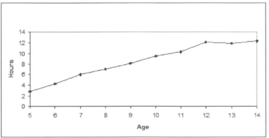
The household questionnaires are constructed to allow the linkage between household members and accomplished domestic activities. It is possible to differ-entiate age and gender patterns in the domestic activities of children, as opposed to agricultural work. There are 12 281 children aged from 5 to 14 years old in the UNHS, divided almost equally between girls and boys, who on average are doing 8.25 hours of non-economic activities per week. Figure 3 presents the evolution of domestic work with children's age.

Children, as they grow older, are more involved in household chores. This upwards trend seems to stop around the age of 12, where the average domestic work time per week is constant for children in the 12 to 14 years old bracket. This increase is quite substantial as children of 12 are doing close to 10 additional hours of domestic activities than children of 5.

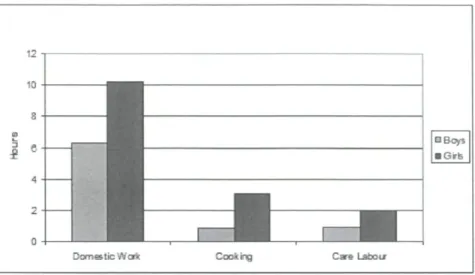
Domestic work can also be studied by gender, as presented in Figure 4, where 27

Figure 3: Age patterns in domestic work per week

girls are more active in household chores. This gender disparity is mainly driven by time spent on cooking related activities, which is three times higher for girls, and more time spent caring for household members.

6 Empirical Application

The first step in studying agricultural production is the choice between a primal approach, centered on a production function, or a dual approach based on cost or profit functions. The estimation of dual approach functions requires information on input and output prices, which are usually imprecise in a developing country. They may vary greatly from one region to another or they may simply be unknown to households. For example, in a community without any form of input or output markets, it is very plausible to encounter many agricultural households who do not trade any of their production. Subsistence farming complicates the use of prices in a formal analysis of agricultural production. Thus, it seems more appropriate to aim towards a primal approach. Cockburn (2001) uses a primal approach to esti-mate children shadow wages and our methodology is largely based on the author's

Figure 4: Gender disparities in domestic work per week

work

6.1 Functional form

The functional form of the production function chosen depends on the desired degree of restrictions. For example, the Cobb-Douglas (CD) functional form is the most commonly used production function however, it assumes a unitary elasticity of substitution between all inputs. The Cobb-Douglas production function at the household level can be expressed in linear form as :

In Yu = a + J 2 &ln Xltk + Bx In LF t + ^ bj X t j + ] T ctuitl + eit (20)

fc J L

where it stands for inputs who vary between households and seasons while i are inputs that vary between households. Y is summed value of crop production, a is the constant and input vector X includes A: productive inputs : adult labor, outside labor, productive assets, material inputs, land cultivated. LF represents child

labor, x a nd v are vectors of household characteristics.16 x contains time invariant

household characteristics : age, education, agricultural knowledge of household head and regional dummy variables. Vector v includes household characteristics that vary between seasons such as self-reported fertility and slope of cultivated plot, self-reported environmental shocks, subsistence dummy, dummy variable for the use of manure, pesticides and improved seed, and a seasonal dummy.17

A functional form like Translog offer more flexibility. Translog production function can be written in the following linear form :

\nYit = a + B1lnLFt + -<f\nLFtlnLFt + -Y/^nLFtlnXk +

k

y~] /3fcln Xitk + er ^ ^ (9ifc In Xia In Xitk + ^ bjXij +

k Ik J

/ ] CiV%a + fit (21)

In both forms, production Y and inputs Xk are expressed in logarithmic form in order to obtain linear equations (20) and (21). Furthermore, the production process differs between households and inputs vector X may have input Xk with a zero value, and this is problematic for the logarithmic transformation. Cockburn (2001) has presented an extended study on production functions and the evalua-tion of child labor, which utilizes various funcevalua-tional forms and treats zero value observations in each of them. The standard approach is to add an arbitrary con-stant to variables that may contain zero value observations. We opt for a method presented in Barrett et al. (2002), which consist of replacing zero value by a con-stant that is equal to a tenth of the smallest strictly positive value taken by input Xk in the sample. This method should be more appropriate than adding a constant

16Adult labor was not divided between male and female adults to maintain a low number of

zero hours spent on agricultural tasks.

17The within-variation comes from the changes of plot cultivated between seasons, which

cre-ates variation at the household level of soil quality and slope.

to the whole distribution of an input, as it should have a smaller effect on input distributions.

On the other hand, there is a functional form called Generalized Cobb­Douglas (GCD) that allows the simultaneous estimation of the additive constants and the input coefficients ( Bl, (3k, bj). The GCD production function for a cross­sectional

analysis can be written simply as :

.7

\nYi = a ­r Y^ PkHXik + ck) + Bx \n{LF + cc) + ^ bj X i j (22)

fc J

where ck and cc are respectively the constant for productive and child labor inputs.

As presented in Soloaga (1999), the estimates can vary quite substantially with the choice of constants. The GCD form can be interesting because the approach could reduce the bias and inconsistency associated with the arbitrary choice of an additive constant.

6.2 Labor elasticity of agricultural production

The labor elasticity of agricultural production is the percentage variation of agri­ cultural output associated with a percentage change in labor inputs. This elasticity can be estimated for every distinct labor input included in the production function. In our case, the labor elasticity corresponds to the variation of production value created by an increase in hours spent on household plots. The production func­ tion is expressed in logarithmic form and this simplify the implementation of the labor elasticity of production as the elasticity is simply the logarithmic variation of production divided by the logarithmic variation of labor : ­^y = j^jr ■

When incorporating a cross­sectional Cobb­Douglas function (20), the labor elasticities are equivalent to the estimated labor coefficients as expressed in the

following equation :

din Y

Bi (23)

d\nLF

Our interest in elasticity relies on the possibility of evaluating the variation of household production associated to child work. With (23), the estimated coefficient B\ can be multiplied with production Yi and divided by the hours worked LF to

obtain the impact of child work on household production. These calculations will estimate the average impact of an increase in child hours worked on household production, which corresponds to the agricultural shadow wage.

Generally, authors have used the marginal productiviy of labor to estimate shadow wages and this methodology was introduced in papers by Jacoby (1993) and Skoufias (1994). However, their method requires a predicted value of pro-duction (Yi) and the first-difference model adequatly captures the difference of production between two seasons but is inadequate to predict the production of each season when they are taken separately. Therefore, to compare the cross-sectional and first-difference estimations, we will be using the labor elasticity to estimate the contribution of children in household production.

The labor elasticity of agricultural production is more complex in the case of Translog production function and can be expressed with the following partial derivative :

dlnYi

l

p = B

+ - ^2 <t>k Inx

+ ip\nL

d \ n LF 2

k

In the case of GCD, the elasticity of labor is simply the coefficient B\ however the constants cc is added to the labor work variable in the estimation of child labor

impact on production, giving the following function :

°* = P-A_ (24)

In the first-difference approach, the labor elasticity of household production is estimated with the following equation :

»N*-1M -Ê, (25)

ein(LJ

-LJ„

The elasticity expressed in (25) uses the difference in production between both seasons as the output, which seems different from the cross-sectional elasticities since the cross-sectional estimates rely on the production at individual seasons. However, since the elasticity is a ratio of percentage variations, the household production from both seasons can be used and even combined for the estimation of elasticities, assuming that there are no major differences in the production process between both seasons. Thus, we will compare the contribution of children on household income regardless of the production variables included in the estimates of elasticities.

The estimate of interest is the elasticity of household production which does not vary between households since it is estimated with a production function. This method will not capture the possible inter-household variations in agricultural labor linked to household characteristics such as productive assets and inputs availability.

6.3 Cross-sectional estimation

The labor elasticities are initially estimated with a cross-sectional approach and compared to the results obtained in the first-difference model. The functional forms CD and Translog are estimated with a ordinary least squares approach whereas the GCD is estimated with nonlinear least-squares. The sample of interest contains the same observations as our first-difference mode, including households who produce during both cropping seasons and use child labor inputs at least once during both

seasons. Household producing in both seasons arc treated as different producing units (i) and the time variance is taken care of by a seasonal dummy.

In the Cobb-Douglas functional form, the impact of adults self-employed labor is higher than outside labor and child labor respectively. The ordinal rank of the three types of labor seems logical as outside laborers are in average as present as child laborer and they would normally be more productive than child workers since they are more likely to be adults. The productive inputs not related to labor have positive and significant effects on household production. As expected, self-reported good soil has a impact on agricultural production. Formal education of household's head and their test score affect production positively. Those variables reflect a certain skill associated with agriculture because households with a relative knowledge of the quality of their land and household heads with more information on agriculture both generate a bigger production. In general, the results of a simple CD production function follow expected beliefs on agricultural production. On the other hand, the interpretation of productive inputs in the Translog for-mulation is more complex as the elasticities of production in regards to productive inputs xk is not simply coefficient 3k- In both functions, households involved in

subsistence farming produce less, OLS regressions capture relatively well the vari-ation in production as R2 is relatively high in both cases. The household head and

soil characteristics follow similar patterns in both functional forms.

The interaction terms included in the TL estimation are presented in Table 3 and the importance of interaction terms can be seen through the joint signifi-cance of the coefficients presented with a F(21,5356) of 14.22. Therefore, the null hypothesis of coefficients jointly equal to zero can be rejected strongly and the Cobb-Douglas form for cross-sectional estimation could be rejected. The individ-ual significance of coefficients is of very little interest and their interpretation is

Table 2: Cross-sectional estimation CD Translog (1) (2) Log(Adult Labor) .240 .005 ( . 0 1 6 ) " * (.121) Log(Child work) .019 .093 (.004)"* (.037)" Log(Outside Labor) .054 .131 (.004)"- (.042)*" Log(Land Area) .268 .045 ( . 0 1 8 ) * " (.142) Log(Productive Assets) .062 -.199 ( . 0 1 2 ) " * ( . 0 7 8 ) " Log(Material Inputs) .009 -.078 (.002)*** (.024)"* Manure .112 .079 (.048)** (.045)* Pesticides .071 -.039 (.053) (.051) Improved Seed .223 .186 ( . 0 3 0 ) * " (.029)*** Good Soil .180 .151 ( . 0 2 9 ) " * (.028)*** Flat Ground -.117 -.105 (.030)"* (.029)*" Major Shock -.045 -.046 (.029) (.028) Subsistence -.732 -.709 (.036)*** (.036)*** Age .002 .001 (.001)* (.001) Male .052 .047 (.031)* (.030) Primary Schooling .117 .120 (.036)*** (.036)*" Secondary Schooling .345 .316 (.045)*" (.044)*** Higher Education .330 .277 ( . 0 5 5 ) " ' ( . 0 5 4 ) " " Test Score .047 .044 ( . 0 0 9 ) * " (.009)*" Seasonal Dummy2005 -.030 -.037 35 (-026) (.026) Constant 9.03 10.5 (.145)*** ( . 6 3 5 ) * " e(N) 5402 5402 e(r2) .489 .516 e(F) 174.273 111.796

Table 3: Translog interaction terms TL (1) Log(Adult Labor)2 .035 ( . 0 0 9 ) * " Log(Child work)2 .008 (.003)*" Log(Outside Labor)2 .024 (.004)*" Log(Land Area)2 -.079 (.019)*" Log(Material Inputs) 2 .024 (.003)*" Log(Productive Assets)2 .027 (.007)*"

Log(Adult Labor) x Log(Child work) -.020

(.008)"

Log(Adult Labor) x Log(Outside Labor) -.037

( . 0 1 0 ) * "

Log(Adult Labor) x Log(Land Area) .064

(.029)**

Log(Adult Labor) x Log(Material Inputs) .0002

(.005)

Log(Adult Labor) x Log(Productive Assets) .013

(.026)

Log(Child work) x Log(Outside Labor) -.006

(.003)"

Log(Child work) x Log(Land Area) .003

(.009)

Log(Child work) x Log(Material Inputs) -.0003

(.001)

Log(Child work) x Log(Productive Assets) -.003

(.007)

Log(Outside Labor) x Log(Land Area) .033

(.011)***

Log(Outside Labor) x Log(Material Inputs) -.002

(.001)

Log(Outside Labor) x Log(Productive Assets) -.004

(.008)

Log(Land Area) x Log(Material Inputs) .001

(.006)

Log(Land Area) x Log(Productive Assets) .010

* .027)

Log(Material Inputs) x Log(Productive Assets) -.002

(.004)

e(N) 5402 F(21,5356) 14.22

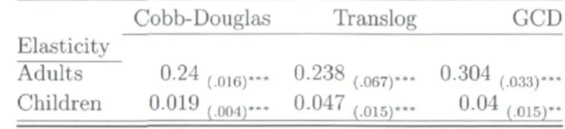
Table 4: GCD estimation

Coefficient Constants (Hours, UGX)

Log(Adult Labor) .304 ( . 0 3 3 ) " * 41.71 (26.31) Log(Child work) .040 ( . 0 1 5 ) " 1.97 (3.31) Log(Outside Labor) .157 ( . 0 3 0 ) " * 24.69 (12.87)*

Log (Land Area) .225

( . 0 1 5 ) " * -.01 (.01) Log(Material Inputs) .426 ( . 1 3 2 ) " " 64 276 (34 457)* Log(Productive Assets) .111 ( . 0 3 0 ) * " 3 228 (3 994) e(N) e(r2) 5398 .508

not especially important as the interaction terms are included to obtain a flexible Translog function in comparison to the relatively restrictive Cobb-Douglas.

In the Generalized Cobb-Douglas estimates presented in Table 4, the major difference lies in productive inputs with a relatively high proportion of zero value inputs, which have higher coefficients than in the CD formulation. This difference is created by the additive constants, which are higher for inputs with a high num-ber of zero observations. The significance of additive constants is questionnable for most of the productive inputs with the exception of outside labor and mate-rial inputs, that arc significant at the 90 percent level. The household head and soil characteristics coefficients are similar to those obtained with the CD and TL formulation and are not presented in Table 4. Cross sectional estimation does not capture significant differences between cropping seasons.

The labor elasticity of child and adult labor in the cross-sectional estimation are expressed in Table 5. A percentage increase in adult labor hours creates an increase of about one quarter of that percentage on household production with the CD