Competitive Insurance Markets and Adverse Selection in the Lab

Texte intégral

(1)2010s-34. Competitive Insurance Markets and Adverse Selection in the Lab Dorra Riahi, Louis Lévy-Garboua, Claude Montmarquette. Série Scientifique Scientific Series. Montréal Août 2010. © 2010 Dorra Riahi, Louis Lévy-Garboua, Claude Montmarquette. Tous droits réservés. All rights reserved. Reproduction partielle permise avec citation du document source, incluant la notice ©. Short sections may be quoted without explicit permission, if full credit, including © notice, is given to the source..

(2) CIRANO Le CIRANO est un organisme sans but lucratif constitué en vertu de la Loi des compagnies du Québec. Le financement de son infrastructure et de ses activités de recherche provient des cotisations de ses organisations-membres, d’une subvention d’infrastructure du Ministère du Développement économique et régional et de la Recherche, de même que des subventions et mandats obtenus par ses équipes de recherche. CIRANO is a private non-profit organization incorporated under the Québec Companies Act. Its infrastructure and research activities are funded through fees paid by member organizations, an infrastructure grant from the Ministère du Développement économique et régional et de la Recherche, and grants and research mandates obtained by its research teams. Les partenaires du CIRANO Partenaire majeur Ministère du Développement économique, de l’Innovation et de l’Exportation Partenaires corporatifs Banque de développement du Canada Banque du Canada Banque Laurentienne du Canada Banque Nationale du Canada Banque Royale du Canada Banque Scotia Bell Canada BMO Groupe financier Caisse de dépôt et placement du Québec Fédération des caisses Desjardins du Québec Gaz Métro Hydro-Québec Industrie Canada Investissements PSP Ministère des Finances du Québec Power Corporation du Canada Raymond Chabot Grant Thornton Rio Tinto State Street Global Advisors Transat A.T. Ville de Montréal Partenaires universitaires École Polytechnique de Montréal HEC Montréal McGill University Université Concordia Université de Montréal Université de Sherbrooke Université du Québec Université du Québec à Montréal Université Laval Le CIRANO collabore avec de nombreux centres et chaires de recherche universitaires dont on peut consulter la liste sur son site web. Les cahiers de la série scientifique (CS) visent à rendre accessibles des résultats de recherche effectuée au CIRANO afin de susciter échanges et commentaires. Ces cahiers sont écrits dans le style des publications scientifiques. Les idées et les opinions émises sont sous l’unique responsabilité des auteurs et ne représentent pas nécessairement les positions du CIRANO ou de ses partenaires. This paper presents research carried out at CIRANO and aims at encouraging discussion and comment. The observations and viewpoints expressed are the sole responsibility of the authors. They do not necessarily represent positions of CIRANO or its partners.. ISSN 1198-8177. Partenaire financier.

(3) Competitive Insurance Markets and Adverse Selection in the Lab* Dorra Riahi†, Louis Lévy-Garboua ‡, Claude Montmarquette§. Résumé Ce travail offre une analyse expérimentale des marchés d’assurance avec anti-sélection. Nous nous intéressons particulièrement aux modèles canoniques d’Akerlof [1970] et de Rothschild et Stiglitz [1976]. Selon Alerlof (1970) l’anti-sélection peut aboutir à une éviction complète des agents les moins risqués. Selon Rothschild et Stiglitz (1976), les contrats de franchise permettent de dépasser cette limite en organisant la sélection des risques : à l’équilibre de marché, les contrats sont spécialisés en fonction des risques individuels. La présente contribution vise à tester ces prédictions théoriques à travers deux expériences de marché d’assurance. Afin de respecter au mieux les hypothèses de base des modèles d’Akerlof et de Rothschild et Stiglitz, nous recourons, dans l’expérimentation, à la technique des loteries binaires. Cette technique génère une neutralité au risque pour les assureurs et une même aversion au risque pour les assurés. Ces expériences sont, à notre connaissance, les premières visant à tester les prédictions des modèles d’assurance avec anti-sélection avec un contrôle des préférences des participants. Les résultats démontrent une éviction partielle des bas risques dans le contexte d’Akerlof (expérience 1). Une éviction qui ne disparaît pas après l’introduction des contrats de franchise (expérience 2). Enfin, à l’opposé de l’équilibre séparateur préconisé par Rothschild et Stiglitz, c’est l’équilibre de pooling qui apparaît (expérience 2). Nous interprétons ces résultats en observant que, dans certaines périodes, certains hauts risques n’achètent pas une assurance complète à un prix inférieur au prix équitable et que certains bas risques achètent une assurance à un prix supérieur à leur volonté induite à payer. Ces résultats robustes sont incompatibles avec la maximisation de l'utilité attendue. La distorsion observée des probabilités conduit à une homogénéisation partielle des risques perçus. Mots clés : économie expérimentale, marché d’assurance, anti-sélection, loterie binaire. *. We owe special thanks to François Pannequin who carefully read the paper. However, we are responsible for all remaining errors. † Ecole Supérieure de Commerce de Tunis, E-mail address: riahi@univ-paris1.fr ‡ Corresponding Author: Centre d’économie de la Sorbonne, Pantheon-Sorbonne University and Paris School of Economics; and CIRANO E-mail address: louis.levy-garboua@univ-paris1.fr § CIRANO, Centre Interuniversitaire de Recherche en Analyse des Organisations. Université de Montréal E-mail address: montmarc@cirano.qc.ca.

(4) Abstract We provide an experimental analysis of competitive insurance markets with adverse selection. Our parameterized version of the lemons’ model (Akerlof 1970) in the insurance context predicts total crowding out of low-risks when insurers offer a single full insurance contract. The therapy proposed by Rothschild and Stiglitz (1976) to solve this major inefficiency consists of adding a partial insurance contract so as to obtain a self-selection of risks. We test the theoretical predictions of these two well-known models in two experiments. A clean test is obtained by matching the parameters of the two experiments and by controlling for the risk neutrality of insurers and the common risk aversion of their clients by means of the binary lottery procedure. The results reveal a partial crowding out of low risks in the first experiment. Crowding out is not eliminated in the second experiment and it is not even significantly reduced. Finally, instead of the predicted separating equilibrium, we find pooling equilibria. We interpret these results by observing that, in any period, some high risks do not purchase full insurance at lower than fair price and some low risks purchase insurance at a price higher than their induced willingness to pay. These robust findings are inconsistent with expected utility maximization. The observed distortion of probabilities leads to a partial homogenization of perceived risks. Keywords: experimental economics, insurance markets, adverse selection, binary lottery procedure, expected utility Codes JEL : C91, D82, G22.

(5) I. Introduction. Akerlof (1970) first identified market failures created by asymmetric information between buyers and sellers regarding the amount of product-specific quality of the goods to be exchanged or the amount of individual-specific risk to be covered. Adverse selection disrupts the market as the better-quality goods or lower-risk individuals are driven out of the market so that only ‘lemons’ are eventually exchanged. The lemons’ model gave rise to a huge literature on the economics of information in search for practical remedies against the inefficiencies generated by informational asymmetries. One of the best known papers in that literature was proposed by Rothschild and Stiglitz (1976) who provide an illuminating solution to the adverse selection problem on competitive insurance markets. If insurers cannot categorize individuals by their exposure to risk, they suggest that a second-best competitive equilibrium can be attained by supplying a menu of insurance policies such that the specific contract freely chosen by each individual reveals his true level of risk. When the proportion of high-risk individuals is relatively high, a separating equilibrium arises, providing for full coverage of high risks and partial coverage of low risks; when the proportion of highrisk individuals falls below a certain threshold, there is no equilibrium. This approach solves the problem raised by the crowding out of low-risk agents through the self-selection of risks. Moreover, it suggests a rationale for the presence of partial insurance contracts (i.e. with a deductible) on insurance markets that is valid in the absence of transaction costs: the deductible provides a risk selection mechanism. The proposals advanced by Akerlof and Rothschild and Stiglitz (RS) subsequently gave rise to a number of further developments (Miyazaki, 1977; Riley, 1979; Spence, 1978; and Wilson, 1977). These approaches, whether or not they allow for the possibility of cross-subsidization between risk classes, provide a very strong rationale for deductibles. While there is a voluminous body of theoretical work on the economics of insurance with adverse selection, empirical applications remain scarce. Furthermore, they come to contradictory conclusions. Some analyses conclude that adverse selection does not appear on the data (Beliveau 1984, Cawley and Philipson 1999, Richaudeau 1999, Chiappori and Salanié 2000, Dionne, Gouriéroux and Vanasse 2001). Others claim that adverse selection is a major problem on insurance markets (Dahlby 1983, Browne and Doerpinghaus 1993, Goodwin 1993, Puelz and Snow 1994, Goodwin and Smith 1995). Consequently, there is no 1.

(6) consensus on either the impact of adverse selection or on the nature of the resulting equilibrium on insurance markets. Furthermore, the lemons’ model has never been empirically tested in the context of insurance for the simple reason that a pure market à la Akerlof –deprived of any corrective mechanisms (deductibles, categorization, bonus-malus, etc.) to prevent the market from collapsing- cannot be observed in the real world because it would vanish as soon as it appears. These issues led us to opt for experimental methods to test the predictions of the Akerlof (1970) and Rothschild and Stiglitz (1976) models. In the controlled environment of a laboratory, we can simulate the working of spot markets repeatedly until a stationary equilibrium emerges or even until the experimental market disappears. Thus, we created an experimental insurance market bringing together three types of agents: insurers, high-risk individuals, and low-risk individuals. In order to be consistent with the simplifying assumptions of models of insurance with adverse selection, participants' preferences were experimentally controlled using the binary lottery procedure originally developed by Roth and Malouf (1979) and subsequently expanded by Berg, Dickhaut and O’Brien (1986), Prasnikar (2000) and Berg, Dickhaut and Rietz (2006). The insurers behave as risk-neutral agents, and the insured individuals behave as risk-averse agents with equal endowments and risk aversion who only differ by their risk level1. Our study focuses on four primary goals: (i) In a first experiment, test the predictions of an adaptation of the lemons’ model to insurance; (ii) In a second experiment, test the predictions of the RS model; (iii) Identify the nature of the equilibria that emerge on competitive insurance markets with adverse selection; (iv) Assess the efficiency of deductibles as a mechanism of risk selection. The related experimental studies are few. It seems that only three experiments have tested the predictions of the RS model. Shapira and Venezia (1999) conducted a separate experimental analysis of supply and demand in a context of insurance with adverse. Recent contributions to the theory have introduced heterogeneity of risk aversion in addition to the heterogeneity of exposure to risk (Landsberger and Meilijson, 1994; Smart, 2000; and Wambach, 2000). Alhough these contributions confirm the role played by deductibles as a mechanism for risk selection, the resulting equilibria are more complex: possibilities of separating, partially separating, and pooling equilibria. These theoretical contributions stress the necessity to control for the degree of heterogeneity in risk aversion. In the absence of such control, our experimental work would offer a test of these recent contributions instead of a test of RS.. 1. 2.

(7) selection. According to their point of view, the first step for a test of the RS model requires to confirm that insureds are inclined to self-selection while insurers are induced to screen their customers. Their experimental data provide partial support to the RS model. The paper of Posey and Yavas (2007) focused on the behaviour of insurers faced to simulated high risk and low risk individuals. Their aim was to test the insurers’ ability to screen their customers in a competitive setting. Depending on the proportions of high risk and low risk individuals on the market, the theoretical prediction is a separating equilibrium (if low risk individuals are relatively few) or a pooling equilibrium (if low risk individuals are relatively many). Posey and Yavas (2007) found a convergence of observed behaviour toward the equilibrium prediction. In the contribution of Asparouhova (2006), the RS model is studied in the context of competitive lending under adverse selection. This experimental analysis is the first one which considers explicitly the interactions between supply and demand. Asparouhova (2006) developed an extension of the RS equilibrium and her experimental results confirm the theory. When the proportion of high risk entrepreneurs is sufficiently high, a separating equilibrium is obtained. When the same proportion is relatively low, lending markets meet difficulties to settle down. Compared to these previous studies, our experiment is the second one involving a true interaction between insurers and insureds. Our main concern was to be in a perfect accordance with the assumptions of the RS model. So, in order to replicate the perfect homogeneity of preferences2, we have selected and gathered together our subjects according to their degree of risk aversion. Finally, an important specificity of our experiment lies in the fact that transactions are not compulsory or automatically implemented. As it is the case in the RS model, insurance contracting is not compulsory and a subject has always the opportunity to refuse it. The originality of our experiments lies primarily in the following. First, no experiment has yet represented both the supply of and demand for insurance in testing both the predictions of Akerlof (1970) or Rothschild and Stiglitz (1976) in this context. Second, no experiment with controls for preferences has been conducted before in the context of insurance. Third, by designing two successive experiments, we are able to assess the effectiveness of deductible contracts as a mechanism for risk selection and as a solution to the problem of adverse 2. In the model of Rothschild and Stiglitz (1976), all individuals are endowed with the same utility function. 3.

(8) selection. To our knowledge, these are the first experiments designed to test the predictions of models of insurance with adverse selection while controlling for the risk preferences of participants. This paper is organized as follows. First we present the theoretical predictions to be tested (Section II). Next, we introduce the experimental protocol in section III and implementation of the binary lottery procedure in section IV. Sections V and VI describe the results of the first and second experiments. We conclude in Section VII.. II. The theoretical predictions to be tested We consider the market supply of an insurance policy to a population composed of two types, H (for high risk) and L (for low risk), that only differ by their probability of loss . Thus,. . These two types are in proportions  H and L respectively,. with H  L  1. The problem of adverse selection arises when insurers know these proportions but cannot observe the risk type of each individual. Individuals are assumed to maximize the expected utility of wealth. With the exception of their risk type, individuals are homogeneous: they are endowed with the same initial wealth W 0 , are at risk of losing the same amount3 X, and share the same concave Von Neumann-. Morgenstern (VNM) utility of wealth function U(W), assumed here to be CARA (Constant Absolute Risk Aversion):. U (W )  eW ,. (1). with α > 0 indicating the degree of absolute risk aversion. Thus, individuals are supposed to be all equally risk averse. The numerical value of  in both experiments is 0.005. On the supply side, we consider a competitive market on which insurers offer insureds, against the payment of a sure premium P, the guarantee to compensate them for a random loss X by an indemnity. (. . Insurers are risk-neutral and maximize their. expected profits. Competition drives profits down to zero and the competitive market premium at which an insurance policy is sold in the absence of transaction costs (loading) is. 3. Individuals are assumed to be unable to influence the probability of a claim or the amount of loss. 4.

(9) the “fair” premium. , where q stands for the average probability of risk among. individuals who are expected to purchase this insurance policy. In the first experiment, which reproduces the lemons’ model, we assume that insurers are unable to discriminate between risk types and compete on the price of a single full insurance policy4. Individual agents only have the option of purchasing full insurance at the market price or no insurance at all. They buy insurance if their expected utility with insurance is at least as great as their expected utility without insurance:. U (W0  P)  (1  qi )U (W0 )  qiU (W0  X ). i  H , L,. The willingness to pay for a full insurance contract (WTP i) of an individual of type i is the maximum premium, that is, with the CARA utility function (1): WTPi . . ln 1  qi (eX  1). .  (2). Thus, if competing insurers supplying full insurance set the insurance premium on the basis of the average probability of loss across all individuals,. , Ls will not buy. insurance if and only if their WTP is below the average fair premium of the whole population, i.e. iff WTPL  qHL.X .. (3). When the latter condition holds, Ls stay out of the market and only Hs buy insurance. Since the average fair premium is lower than the high risk fair premium, insurers' profits are negative. The policy will be withdrawn and replaced with a new policy that targets type H individuals. Adverse selection would thus restrain the supply of insurance to a contract offering full insurance at a fair price for Hs. At this price, Ls are crowded out of the market, insurers compete exclusively for Hs, and competition drives profits down to zero. This is the prediction we wish to test with the first experiment. For this purpose, condition (3) is imposed on our data. Letting. =0.50,. , fair. premiums amount to 20 for Ls, 60 for Hs, and 40 on average; since. ,. condition (3) is respected.. 4 In this experiment, the observed price p and premium P of an insurance contract may be confounded because they remain proportional: .. 5.

(10) In the second experiment, which reproduces the RS model, we still assume that insurers are unable to discriminate between risk types but they now compete on a menu of contracts which includes a full insurance policy and a partial insurance policy. Since the VNM utility function of all individual agents is given by (1), we are able to compute the menu of profitable incentive-compatible policies that allows low risks to get the best coverage and high risks to be separated from low risks under the model’s assumptions. Each insurer proposes a policy with a deductible D appealing to Ls and a full insurance policy appealing to Hs. In this separating equilibrium, competition drives profits down to zero on both contracts. Thus, the full insurance premium is fair to its H clients:. PF  qH  X. (4). and the deductible policy premium is also fair to its L clients:. PD  qL .( X  D). (5). Ls self-select the partial insurance policy, and this policy allows them to maximize their expected utility under the constraint that high risks self-select the full insurance policy:. U (W0  PF )  (1 qH )U (W0  PD )  qHU (W0  PD  D) Thus, the last constraint is saturated, and, with CARA utility function (1), the optimal deductible D offered to Ls is the solution of:. . ln 1  q H (e D  1). . Or, using (2), (4), (5):. . (6). (D). Thus, the excess premium paid by Hs to get full insurance rather than partial insurance equals their WTP for the coverage of deductible D. With the CARA utility function (1), =0.40,. we. compute:. . However, a separating equilibrium can only obtain if partial insurance for Ls at fair price dominates pooling contracts at an average fair price, that is, if the proportion of high risks is sufficiently large. With our experimental parameters, . If there are not enough high risks, the RS model has no equilibrium. The equilibrium value of deductible is imposed on the data and the chosen proportion of Hs. 6.

(11) (60%) is well above the computed threshold value. The theoretical prediction we wish to test in the second experiment is that a separating equilibrium obtains at fair prices, with Hs purchasing the full insurance contract and Ls purchasing the partial insurance contract while insurers make no profit on both contracts.. III Experimental Design a) General features: The two experiments were conducted in Bell University Laboratories' experimental economics centre at CIRANO in Montreal, using the Ztree software (Fischbacher 2007). We ran five sessions in the first experiment and six in the second. Each session consists of an insurance market with “clients” and with “insurers” competing on prices. The allocation of the roles insurer/client is determined by a random draw at the beginning of the experiment and the roles assigned to the participants do not change throughout the session. Each insurance market is made up of sixty trading periods. This relatively long time-horizon was chosen to facilitate the emergence of a stationary equilibrium. The currency used for transacting is the experimental money unit (EMU). At the beginning of each trading period, every insurer receives an initial endowment of 5000 EMU, which makes it possible to cover all contingencies. All potential insureds receive the same initial endowment, equal to 1000 EMU, regardless of their risk profile. The supply of insurance is provided by four insurers who compete on prices5. The trading mechanism adopted in both experiments corresponds to the institution of posted prices. 6 The demand for insurance emanates from two risk types: high risk and low risk clients, who are indistinguishable to insurers. Each high risk (H) has a 30% probability of losing 200 EMU, and each low risk (L) has a 10% probability of losing the same amount. Thus, the fair premium reached under perfect competition is 60 EMU for Hs and 20 EMU for Ls. In the first experiment, the demand for insurance comes from four high-risk and four lowrisk clients who have a choice between full insurance (F) and no insurance (N). In the second 5. All experiments that previously tested the institution of posted auctions indicate that competitive prices will only be obtained systematically with three sellers at least, even though, in theory, Bertrand competition allows competitive prices to be attained with as few as two sellers. 6 Holt (1995: 375) recommends the use of posted prices for the experimental simulation of competitive insurance markets. 7.

(12) experiment, the demand for insurance comes from six high-risk and four low-risk clients7 who have the two same choices (N, F) and an additional choice of partial insurance with a deductible (D). When a loss occurs, clients get a full coverage of 200 EMU if they chose full insurance, only 60 EMU – that is, 200 EMU minus a deductible of 140 EMU- if they opted for partial insurance and nothing if they didn’t purchase insurance. The deductible was derived from a numerical version of the RS model in which all clients have a CARA utility function (1) with. .. Each session is divided in three steps. The first consists of training questions for the participants to familiarize themselves with the experimental protocol. The second corresponds to the experiment itself. Finally, during the third step, the participants are compensated. Participants' earnings depend partly on decisions made during the game and partly on luck. Compensation is distributed individually at the end of the experiment. Participants earned an average of twenty-five Canadian dollars in one-and-a-half hour. b) the trading periods: Each trading period of an experiment involves three stages. First stage: In the first stage, insurers compete for the lowest premium of each contract they may offer: a full insurance contract (F) only in the first experiment; or a full insurance (F) and a partial insurance contract with a deductible (D) in the second experiment. The insurer with the lowest insurance premium will be the only one to sell policies during the active trading period. If two insurers at least offer the same premium in a given trading period, the computer determines which one will sell insurance by a random draw. There are no transaction costs, but insurers are free to fix the premiums above or below their actuarial level. Second stage: Each client is informed of the amount of the market premium for each contract, that is, F in the first experiment, and (F, D) in the second. Then, she must choose her preferred insurance policy or no insurance (N). 7. Given the preferences induced by the binary lottery procedure, we mentioned in the previous section that the separating menu (F,D) is an equilibrium iff the proportion of high risks exceeds 12%. The selected proportion of 60% considerably exceeds this threshold.. 8.

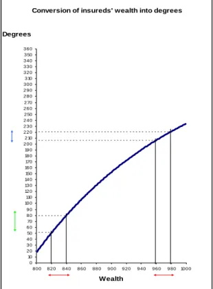
(13) Third stage: A lottery determines which clients suffer losses. The computer then computes the final endowment of each client and insurer, and displays it on screen. Each insurer is informed of how many policies of each type she sold, the claims she must pay, the profit yielded by each policy, and her endowment at the end of the trading period. Uninsured clients pay no premium and totally cover their own losses. In contrast, insured clients pay insurance premiums and receive indemnities from their insurer if they suffered a loss. From the insurers’ perspective, profits increase their endowment, while from the clients’ perspective, premiums and uncovered losses reduce their endowment. III. Implementation of the binary lottery procedure a) Compensation to participants: Participants are compensated on the basis of the earnings (in EMU) obtained at the end of one of the 60 trading periods, randomly selected by computer at the end of the experiment. All trading periods have an equal likelihood of being drawn. However, subjects do not receive their earnings as payments. The binary lottery procedure that we use to control for their risk attitude8 requires that each participant may only win one of the two following prizes: the "high prize," equal to can$30, or the "low prize," equal to can$10. The more a participant earns at the end of the selected trading period, the higher will be his likelihood of winning the high prize. Indeed, each level of final wealth corresponds with a number of degrees on a wheel which determines, by proportionality, the probability of winning. There are two different wheels for insurers and for clients. For insurers, the function that translates wealth into degrees is linear and implies risk neutrality: Degrees  360[(W  4000) 2000]. 8. Previous applications of the binary lottery procedure in experiments are Berg, Dickhaut and O’Brien (1986) on. decision-making under risk, Rietz (1993) and Walker, Smith, and Cox (1990) on auctions, Roth and Malouf (1979) on game-theoretic models of bargaining, and Dittrich, Güth and Maciejovsky (2005) on investment. Surprisingly, to our knowledge the binary lottery procedure had never been applied to insurance.. 9.

(14) where W indicates total earnings at the end of the selected trading period. For clients, the function translating earnings into degrees is CARA and implies a constant absolute risk aversion equal to 0.005: Degrees  360  360e0.005(W 790). Participants do not see these functions but either figure 1 or figure 2, indicating the conversion of their potential earnings into degrees according to their role in the experiment. They could also consult a conversion table containing precise numerical values. Conversion of insureds' wealth into degrees. Degrees Conversion of insurers' wealth into degrees. 360 350 340 330 320 310 300 290 280. Degrees 360 350 340 330 320 310 300 290 280 270 260 250 240 230 220 210 200 190 180 170 160 150 140 130 120 110 100 90 80 70 60 50 40 30 20 10 0 6900. 6600. 6300. 6000. 5700. 5400. 5100. 4800. 4500. 4200. 3900. 3600. 3300. 3000. 270 260 250 240 230 220 210 200 190 180 170 160 150 140 130 120 110 100. Wealth. Figure 1: Conversion of insurers' wealth into degrees. 90 80 70 60 50 40 30 20 10 0 800. 820. 840. 860. 880. 900. 920. 940. 960. 980. 1000. Wealth. Figure 2: Conversion of insureds' wealth into degrees. 10.

(15) Once the experimenter knows the participant’s probability of winning and has delimitated her winning zone on the appropriate wheel, the latter spins the arrow on the wheel clockwise. If the arrow comes to rest in the winning zone, she wins Can$30. If the arrow lands outside of the winning zone, the earnings are only Can$10. Figure 3 illustrates these two scenarios.. 0. Prize wheel. 0. Arrow. Boundary of the winning zone. Participant wins $30 participant gagne 30$. Boundary of the winning zone. Participant wins $10mite de la $10 $10Le participant zone gagnante gagne 10$. Figure 3 : The Prize Wheel and two scenarios. b) Does the binary lottery procedure control for risk aversion? Before showing the results, we wish to check that we effectively control for the risk attitude of clients with the binary lottery procedure9. For this purpose, we administered the Holt and Laury’s (2002) procedure to our subjects at the beginning of each experiment in order to establish their risk attitude. Every participant had to choose ten times between two options A and B, each of which corresponds to a binary lottery with payoffs. A is a safe bet with payoffs can$4 and can$3.20 and B is a risky bet with payoffs can$7.70 and can$0.20. Probabilities of the higher payoffs are equal for the two lotteries and vary by steps of 0.10 from 0.10 to 1.00. Normally, subjects switch once from A to B for one value of this probability and the number of safe choices serves as an index of risk aversion. Values between 0 and 3 indicate risk loving, an index of 4 signals risk neutrality, and values between 5 and 9 indicate risk aversion. We gave participants an incentive to reveal their true risk attitude by telling them that one of the ten choices made would be randomly selected and 9. Risk neutrality was also imposed on insurers by the same procedure. We shall test, in subsection IV (result 2) and V (result 5), that insurers effectively compete and make no profit. 11.

(16) played for money. On average, they received can$5.35 for this task. We first checked by a Kruskal-Wallis test that we could not reject the hypothesis that the four distributions of risk attitudes (number of safe choices) in ten categories across experiments (1 and 2) and risk types (H and L) were identical (  2 =0.516; Prob=0.9154). Then, we divided each of the four samples in two broader categories of roughly equal size: 1) Non risk averse (ie., risk neutral and risk loving); 2) Risk averse. In order to examine whether the binary lottery procedure has allowed us to equalize the risk preferences of clients, we compared the choice frequencies of insurance contracts between these two categories of risk attitude. In both experiments, a Wilcoxon signed-rank test reveals that the average frequency of choices of insurance does not differ significantly between the two categories of risk attitude. In the first experiment, the test results are (z = 0.566; Prob > |z| = 0.5716) for Hs and (z = -1.483; Prob > |z| = 0.1380) for Ls; and, in the second experiment, they are (z = -0.863; Prob > |z| = 0.3883) for Hs and (z = 1.054; Prob > |z| = 0.2918) for Ls. These results show that the binary lottery technique allowed us to control for the risk attitude of clients in both experiments. In the following we consider that participants' risk preferences are controlled for and that our experiments offer a clean test of the classical models of competitive insurance markets with adverse selection proposed by Akerlof (1970) and Rothschild and Stiglitz (1976). The nonparametric analyses will primarily be based on average choices made by insurers (premiums) and clients (choice of insurance) in each of the independent sessions. For each test, we require a confidence level of no less than 95%.. IV Results of the first experiment We first test on the five sessions of our first experiment (one policy) the following predictions of the lemons’ model of competitive market with adverse selection: P1.1: The market premium equals (converges toward) the fair premium of Hs. P1.2: Insurers make no profit. P1.3: No Ls and all Hs buy insurance. Result 1: In three sessions of the one-policy experiment, the market premium converges toward the average fair premium for the total population. In one session, it converges. 12.

(17) toward the fair premium of Ls. And in one session only, it converges toward the fair premium of Hs as the theory predicts. Result 1, shown on figure 4, largely contradicts the first theoretical prediction. In a majority of sessions, the market premium converges toward the average of Hs’ and Ls’ fair premiums in about 15 periods. This holds too when the five sessions are aggregated. A Wilcoxon signed-rank test then reveals that the insurance premium offered per session does not significantly differ from the mean fair premium for the total population (z = –0.674; Prob > |z| = 0.5002). Figure 4: Three scenarios of convergence of the market premium Average premiums Sessions: 1, 3 and 5 160 140. average premium. 120. average actuarial premium of total population. 100. high risks actuarial premium. 80 60. low risks actuarial premiums. 40 20 0 1. 4. 7 10 13 16 19 22 25 28 31 34 37 40 43 46 49 52 55 58 Periods. (4.a) Average fair premium of total population Naïve scenario Session 2. 160 140. average premium. 120 average actuarial premium of total population. 100 80. high risks actuarial premium. 60 low risks actuarial premiums. 40 20 0 1 4 7 10 13 16 19 22 25 28 31 34 37 40 43 46 49 52 55 58 Periods. (4.b) Fair premium of Ls. 13.

(18) Akerlof's scenario Session 4 160 140. average premium. 120 average actuarial premium of total population. 100. high risks actuarial premium. 80 60. low risks actuarial premiums. 40 20 0 1. 4 7 10 13 16 19 22 25 28 31 34 37 40 43 46 49 52 55 58 Periods. (4.c) Fair premium of Hs The first two scenarios are surprising as they seem to invalidate the theoretical prediction (see section 2) that, in the present experimental conditions, adverse selection would restrain the supply of insurance to a contract offering full insurance at a fair price for Hs. An immediate answer to this finding is that insurers might be predominantly naïve, and target the whole population if they don’t observe their clients’ risk type on an individual basis. However, by condition (3), only Hs should get insurance at this price, so that profits should be negative under these scenarios. Therefore, we would expect boundedly rational insurers to be naïve in the first trading periods and revise their strategy after experiencing repeated losses. However, such interpretation is not supported by the data. The insurance premium in the first period has a mean value of 80, well above the average fair premium of 40, and shows considerable variation across sessions10. Moreover, premiums do not converge toward the high-risk fair premium value of 60, but toward the average fair premium value of 40. Dividing the sixty-period interval in two thirty-period intervals I1 and I2, the premium remains stable and does not significantly diverge from the average fair premium of the two risk types, both on interval I1 (z = –0.674; p-value = 0.5002) and I2 (z = –0.405; p-value = 0.6858). Thus, we are confronted with a puzzle: insurers lack information on the risk type of their clients but they are not particularly naïve; yet, they offer in the long run a “low” premium that should take them into repeated losses. Result 2: The profits earned by insurers who cannot offer more than one policy are not significantly different from zero.. 10. The first-period premiums observed in the five sessions were respectively: 50, 40, 10, 150, 150. 14.

(19) Result 2 solves the puzzle that we just raised by showing that insurers effectively maximize their expected profit and, under perfect competition, earn zero profit. The latter hypothesis cannot be rejected by a Wilcoxon signed-rank test (z = –0.098; p-value = 0.9221). Moreover, mean profits per period were non-significantly different from zero in the five sessions11. Thus, markets were competitive in all the sessions and the second theoretical prediction is verified. In order to verify the third theoretical prediction in the context of the first experiment, we compare the average frequencies of insurance purchase during each of the intervals I1 and I2. Ls would be “crowded out” of the insurance market if they purchase coverage less frequently in I2 than in I1, and crowding out would be “total” if their frequency of coverage in I2 is not significantly different from zero. Result 3: When insurers cannot offer more than one policy, Ls are crowded out of the insurance market under adverse selection. However, some Ls do not leave the market and some Hs do not enter the market. An application of the Wilcoxon test to the percentage of insurance policies purchased by low risks in each interval I1 and I2 reveals that, while the latter are crowded out of the insurance market (z = 2.023; p-value = 0.0431), the mean proportion of low risks insured in each session during the final thirty periods (I2) is significantly different from zero (z = 2.023; pvalue = 0.0431). Looking now at high risks, Wilcoxon signed-rank tests show that they buy insurance as much in I2 as in I1 (z = 0.944; p-value = 0.3452) and they purchase coverage more frequently than low risks (z = 2.023; p-value = 0.0431). The last result confirms that adverse selection reduced the opportunities for insurance available to Ls compared to those available to Hs. A question remains: In four out of the five sessions, insurers charged a premium lower than the fair premium of Hs although Ls were crowded out and Hs outnumbered Ls on the market. How can insurers not suffer losses under such conditions? The answer to this question lies in a simple fact: in any period, some Hs do not purchase full insurance at lower than fair price and some Ls purchase insurance at a price higher than their WTP. Indeed, a Wilcoxon signed-rank test shows that a significant proportion of Hs did not purchase 11. The mean profits observed in the five sessions were respectively: -13, -29, -31, +3, -25. These values are to be compared with an initial endowment of +5000. 15.

(20) insurance when the market premium was lower than WTPH. (z=-2.023; p-. value=0.0431). Conversely, a significant proportion of Ls bought insurance when the market premium was higher than WTPL (z= 2.023; p-value=0.0431). These two results do not change if the 15 first periods -that is, before the stationary equilibrium is reached- are taken out of the sample. Since the use of the binary lottery procedure effectively controls for risk aversion (see subsection III b), such observation is inconsistent with the maintained assumption that our experimental clients are EU maximizers. We may further say that subjects violated EU by distorting objective probabilities of loss. It strikes us that EU theory was violated in spite of the large experience that our subjects had the opportunity to acquire on their experimental market. On average, high risks perceived less than 30% risk of loss and low risks perceived more than 10% risk of loss, which resulted in a partial homogenization of risk types. Consequently, insurers were able to reduce the price of insurance below the fair price of Hs. Figure 5 illustrates all these results in more detail by showing how the demand for insurance evolves over time for Hs and for Ls in the three types of sessions:. Figure 5: Partial crowding out of low risks and retention of high risks Main scenario Sessions: 1, 3 and 5. 100% 90% 80% 70% 60% 50% 40% 30% 20% 10% 0%. Average percentage of insured high risks. Average percentage of insured low risks. 1. 5. 9. 13 17 21 25 29 33 37 41 45 49 53 57 Periods. (5.a) Sessions in which the premium converges toward the average fair premium of total population. 16.

(21) Naive scenario Session 2. 100% 90% 80% 70% 60% 50% 40% 30% 20% 10% 0%. Average percentage of insured high risks. Average percentage of insured low risks. 1. 5. 9. 13 17 21 25 29 33 37 41 45 49 53 57 Periods. (5.b) Session in which the premium converges toward the fair premium of Ls Akerlof-type Scenario Session 4. 100% 90% 80% 70% 60% 50% 40% 30% 20% 10% 0%. Average percentage of insured high risks. Average percentage of insured low risks. 1. 5. 9 13 17 21 25 29 33 37 41 45 49 53 57 Periods. (5.c) Session in which the premium converges toward the fair premium of Hs. The picture described in the majority of sessions (figure 5.a) is a reflection of the aggregate results previously discussed. Figures 5.b and 5.c are of special interest. In session 2 (5.b), the premium converged toward the fair premium of Ls because Hs were particularly reluctant to buy full insurance in that session. Consequently, insurers were able to cut prices in order to attract Ls. Figure 5.b shows that the proportion of Ls buying insurance in that session was about as high as that of Hs. Session 4 (5.c) is the only one for which the premium converges toward the fair premium of Hs, as EU theory would predict here. Obviously, Hs were particularly prone to buy insurance in that session, which led insurers to raise prices. Figure 5.c shows then that Ls were crowded out of the market.. 17.

(22) V. Results of the second experiment Assuming that individuals only differ by their risk type, Rothschild and Stiglitz (1976) suggested that introducing a partial insurance policy in addition to the full insurance policy would circumvent the crowding out of low risks in a competitive insurance market if the proportion of high risks is large enough. Our second experiment respects the latter condition and tests the following theoretical predictions delineated in section 2: P2.1: A separating equilibrium obtains at fair prices, with Hs purchasing the full insurance contract and Ls purchasing the partial insurance contract; P2.2: Insurers make no profit; P2.3: low risks are not crowded out of the insurance market. Result 4: A pooling equilibrium can be observed in four sessions out of six on the two insurance contracts. Full insurance is offered at the average fair premium of the total population and purchased by both risk types; partial insurance is offered at a price which lies between the fair premium of Ls and the average fair premium and purchased by both risk types as well. Two partially separating equilibria are also observed in the two remaining sessions. In one session, full insurance is purchased by the two risk types and partial insurance is purchased exclusively by Ls. In another session, the full insurance policy is bought exclusively by Hs and the partial insurance policy is shared by the two risk types. Result 4 can be visualized on figure 5. It means that most of the observed equilibria are not separating but rather pooling equilibria, which contradicts the theoretical prediction. Although recent contributions to the theory predict similar possibilities of separating, partially separating, and pooling equilibria when two sources of heterogeneity coexist, both on the level of risk and on risk aversion (Landsberger and Meilijson, 1994; Smart, 2000; and Wambach, 2000), controlling for risk aversion as we did should have ruled out such possibilities. Of course, other equilibrium concepts (Miyazaki, 1977; Riley, 1979; Spence, 1978; and Wilson, 1977) have also been introduced with a single source of heterogeneity (risk level). However, the pooling equilibrium is only predicted by Wilson’s (1977) model when the proportion of high risks on the insurance market is small, so that it should not be observed here given the great proportion of high risks in our experiments. Moreover, the 18.

(23) two contracts that would have been predicted by the RS model conditional on the (controlled) risk aversion of clients and proportion of Hs were imposed on the data (as in Posey and Yavas 2007); and this also seems likely to favour the emergence of the RS equilibrium. Finally, notice that we do not observe the separating equilibria with crosssubsidization between risk types predicted by Miyazaki (1977), but not by the RS model, although insurers were free to set the premiums at their preferred level. This may be the result of coordination failure among insurers when the whole supply of each insurance policy is attributed competitively in each period to the lowest bidder.. Figure6: Three scenarios of equilibrium for partial and full insurance Pooling for complete insurance Sessions: 1, 3, 4 and 6 160. Pooling for partial insurance Sessions 1, 3, 4 and 6 Average premium. 140. 60. Average premium. 50. 120. High risk's actuarial premium. 100. High risk's actuarial premium. 40 30. 80. Low risk's actuarial premiums. 60 40. Average actuarial premium of all population. 20 0 1. 4. Low risk's actuarial premiums. 20 10. Average actuarial premium of all population. 0 1. 7 10 13 16 19 22 25 28 31 34 37 40 43 46 49 52 55 58. 4. 7 10 13 16 19 22 25 28 31 34 37 40 43 46 49 52 55 58. Periods. Periods. (a) Pooling for partial and full insurance Separation for complete insurance Session 5. Pooling for partial insurance Session 5 60. 160 140 120 100 80 60 40 20 0. Average premium High risk's actuarial premium Low risk's actuarial premiums Average actuarial premium of all population 1. 4. Average premium. 50 High risk's actuarial premium. 40 30. Low risk's actuarial premiums. 20 10. Average actuarial premium of all population. 0 1. 7 10 13 16 19 22 25 28 31 34 37 40 43 46 49 52 55 58. 4. 7 10 13 16 19 22 25 28 31 34 37 40 43 46 49 52 55 58 Periods. Periods. (b) Separation for full insurance and pooling for partial insurance Pooling for complete insurance Session 2 160. Seperation for partial insurance Session 2 Average premium. 140 120. 60. Average premium. 50 High risk's actuarial premium. 100. 40. 80 60. Low risk's actuarial premiums. 30. 40 20. Average actuarial premium of all population. 10. 0. High risk's actuarial premium Low risk's actuarial premiums. 20. Average actuarial premium of all population. 0 1. 4. 7 10 13 16 19 22 25 28 31 34 37 40 43 46 49 52 55 58 Periods. 1. 4. 7 10 13 16 19 22 25 28 31 34 37 40 43 46 49 52 55 58 Periods. (c) Pooling for full insurance and separation for partial insurance. The equilibrium obtained in the majority of sessions also emerges when all sessions are aggregated. The full insurance premium then converges toward the average fair premium of. 19.

(24) the total population (z –1.153; p-value = 0.2489). The supply of full insurance is not targeted at Hs but based on a pooling of risks. Similarly, the supply of partial insurance is not exclusively targeted at Ls: a Wilcoxon signed-rank test reveals that the average premiums of deductible-based policies offered between sessions are higher than the fair premium of Ls (z = 2.201; p-value = 0.0277) and lower than the mean fair premium of the total population (z = –2.201; p-value = 0.0277). Nonetheless, a greater proportion of Ls than Hs purchase the partial insurance policy. Convergence toward the two stationary values is fast since market premiums required for full coverage (I1 vs. I2: z = 0.314; p-value = 0.7532) and for partial coverage (I1 vs. I2: z = 0.734; p-value = 0.4631) appear to be stable over time. In conclusion, data from the second experiment refute Prediction P2.1, according to which each insurance policy is tailored to a risk type. Instead, they reflect a strategy of pooling by insurers. Result 5: The profits earned by insurers on each contract are not significantly different from zero. Application of the Wilcoxon signed-rank test reveals that we cannot reject the null hypothesis, according to which the profits earned both on the full insurance policy and on the partial insurance policy are nil (F policy: z = –1.414; p-value = 0.1574. D policy: z = –1.241; p-value = 0.2144). Thus, insurers behave as expected profit maximizers under perfect competition. Furthermore, they manage to pool risks and avoid losses. Result 6: Hs prefer full coverage and Ls are indifferent between full coverage and a deductible. Ls are still crowded out of the market when they have a choice between two insurance policies. A Wilcoxon signed-rank test on the mean number of insurance policies purchased during each session reveals that Hs acquired more F than D policies (z = 2.201; p-value = 0.0277) while Ls acquired an equal number of F and D policies (z = -1 363; p-value = 0.1730). These behaviors remained stable over time.. 20.

(25) Evolution of High risks' insurance choices. 100% 90% 80% 70% 60% 50% 40% 30% 20% 10% 0%. First thirty periods I1. 52%. 46% 25% 24%. Full Insurance. Partial Insurance. 30% 23%. Second thirty periods I2. No Insurance. Figure 7: The distribution of insurance choices of high risks over time Evolution of Low-risks insurance choices 100% 90% 80% 70%. 61%. First thirty periods I 1. 60%. 43%. 50%. 37%. 40% 30% 20%. 29% Second thirty periods I 2. 20% 10%. 10% 0% Full insurance. Partial insurance. No insurance. Figure 8: The distribution of insurance choices of low risks over time. Thus, self-selection of Hs on full insurance yields some support to the RS predictions while the weakness of self-selection of Ls on partial insurance invalidates them, as Figures 7 and 8 demonstrate. Another result shown by Figure 8 is even more striking: Ls purchase no insurance at all half of the time. More precisely, Ls are crowded out of the insurance market since they buy more insurance in I1 than in I2 (z = 2.201; p-value = 0.0277). This last result concerns both insurance policies. A higher proportion of Ls chose full insurance in I1 than in I2 (z = 1.782; p-value = 0.0747), and the same goes for the deductible policy (z = 2.201; pvalue = 0.0277). Thus, low risks learn to shun both insurance contracts, as Figure 8 reveals.. 21.

(26) In conclusion, the introduction of deductible contracts only gave rise to partial self-selection of individuals and, above all, it didn’t stop the crowding out of low risks. By offering differentiated policies, insurers allow low risks to buy insurance at fair prices. Thus, even though low risks have fewer opportunities to buy insurance than they would under symmetry, policies with a deductible should allow them to remain on the insurance market. Our experimental results refute this proposition: the (per session) average percentage of insured Hs is significantly above that of insured Ls (z = 2.201, p-value = 0.0277). Overall, 73% Hs get some kind of insurance versus 48% Ls only. Result 7: The rate at which Ls are crowded out of the insurance market has not been significantly reduced by the RS therapy. The crucial test yielding this result is based on a direct comparison of our two experiments in which all equilibrium-relevant parameters were given the same value. The rate of crowding out of Ls reaches a high of 68% in the first experiment and a low of 52% in the second. However, the difference is not significant by a Mann-Whitney U test (z = 1.464; p-value = 0.1432). This finding is illustrated by Figure 9: Crowding out of low risks 100% 90% 80% 70%. 68%. 60%. 52%. 50%. Crowding out of low risks Experience 1 Crowding out of low risks Experience 2. 40% 30% 20% 10% 0%. Crowding out of low risks Experience 1. Crowding out of low risks Experience 2. Figure 9: The crowding out of low risks in the two experiments. VI.. Conclusion. This paper has presented an experimental analysis of competitive insurance markets with adverse selection focusing on the canonical models of Akerlof (1970) and Rothschild and Stiglitz (1976). The first experiment was designed such that low-risk agents would be crowded out when a single full insurance contract can be offered but insurers cannot. 22.

(27) observe the risk type of their clients. The second experiment allowed the supply of the two levels of coverage predicted by the RS model while leaving competition set the market prices. Repeated experimental spot markets are especially suited to observe a disappearing ‘market for lemons’ and to control for exposure to risk, adverse selection, the number and type of insurance contracts, the absence of loading, and perfect competition. Our experiments offer the closest experimental description of competitive insurance markets so far in the literature. In addition, they present two unique features worth mentioning. First, the binary lottery procedure was used to (successfully) control for the risk neutrality of insurers and the common risk aversion of clients. Second, the parameters of both experiments were matched in order to provide a clean test of the RS therapy of supplying two specific contracts instead of one for stopping the crowding out of low risks. The results reveal a partial crowding out of low risks when a single full insurance contract can be offered (experiment 1). Crowding out is not eliminated and it is not even significantly reduced by the introduction of deductible contracts (experiment 2). Finally, in contrast to the predicted separating equilibrium, we find pooling equilibria (experiment 2). The maintained assumption of expected utility underlying classical models does not appear to obtain for participants in their choice of insurance. Pooling equilibria can be sustained because insureds who objectively differ in their risk level do not perceive themselves as being so much different.. References: Akerlof, G. (1970) “The Market for Lemons: Quality Uncertainty and the Market Mechanism” Quarterly Journal of Economics 84, 488-500. Asparouhova, E. (2006) “Competition in Lending: Theory and Experiments”, Review of Finance 10, 189-219. Beliveau, B. (1984) “Two Aspects of Market Signaling”, Unpublished Ph. D. thesis, Yale University, New Haven: Connecticut. Berg, J.E., L.A. Daley, J.W. Dickhaut and J.R. O'Brien (1986) "Controlling preferences for lotteries on units of experimental exchange," Quarterly Journal of Economics 101, 281-306. Berg, J. E., J. W. Dickhaut and T. A. Rietz (2006) “On the Performance of the Lottery Procedure for Controlling Risk Preferences,” in C.R. Plott and V.L. Smith (eds.), Handbook of Experimental Economics Results (New York: Elsevier Press).. 23.

(28) Browne, M. J., and H. J. Doerpinghaus (1993) “Information Asymmetries and Adverse Selection in the Market for Individual Medical Expense Insurance”, Journal of Risk and Insurance 60, 300-312. Cawley, J., and T. Philipson (1999) “An Empirical Examination of Information Barriers to Trade in Insurance”, American Economic Review 89, 827-846. Chiappori, P.A. and B. Salanié (2000) “Testing for Asymmetric Information in Insurance Markets”, Journal of Political Economy 108, 56-78. Dahlby, B.G. (1983) “Adverse Selection and Statistical Discrimination”, Journal of Public Economics 20, 121-130. Dionne, G., C. Gouriéroux, and C. Vanasse (2001) “Testing for Evidence of Adverse Selection in the Automobile Insurance Market: A Comment”, Journal of Political Economy 109, 444-453. Dittrich, G. and B. Maciejovsky (2005) “Overconfidence in Investment Decisions: an Experimental Approach,” The European Journal of Finance 11, 471-491. Fischbacher, U. (2007) “z-Tree: Zurich Toolbox for Ready-Made Economic Experiments”, Experimental Economics 10, 171-178. Goodwin, B. (1993) “An Empirical Analysis of the Demand of Multiple Peril Crop Insurance”, American Journal of Agricultural Economics 75, 425-434. Goodwin, B. and V. Smith (1995) “Economics Of Crop Insurance and Disaster Aid”, AEI Studies in Agricultural Policy. Holt, C. (1995) Handbook of Experimental Economics, Princeton, N.J.: Princeton University Press. Holt, C. and S. Laury (2002) “Risk Aversion and Incentive Effects”, American Economic Review 92, 1645-1655. Landsberger, M. and I. Meilijson (1994) “Monopoly Insurance under Adverse Selection when Agents Differ in Risk Aversion”, Journal of Economic Theory 63, 392-407. Miyazaki, H. (1977) “The Rat Race and Internal Labor Markets”, Bell Journal of Economics 8, 394-418. Posey, L. and A. Yavas (2007) “Screening Equilibria in Experimental Markets,” The Geneva Risk and Insurance Review 32, 147-167. Prasnikar, V. (2000), “Binary Lottery Payoffs: Do They Control Risk Aversion?”, Mimeo, Carnegie Mellon University. Puelz, R. and A. Snow (1994) « Evidence on Adverse Selection: Equilibrium Signaling and CrossSubsidization in the Insurance Market », Journal of Political Economy 102, 236-257. Richaudeau, D. (1999) “Automobile Insurance Contracts and Risk of Accident: An Empirical Test Using Individual Data”, Geneva Papers on Risk and Insurance Theory 24, 97-114. Riley J. G. (1979) “Informational Equilibrium”, Econometrica 47, 331-359. Rietz, T. A. (1993) “Implementing and Testing Risk-Preference Induction Mechanisms in Experimental Sealed-Bid Auctions,” Journal of Risk and Uncertainty 7, 199-213. Roth, A.E. and M.W.K. Malouf (1979) “Game-Theoretic Models and the Role of Bargaining”, Psychological Review 86, 574-594.. 24.

(29) Rothschild, M. and J. Stiglitz (1976) “Equilibrium in Competitive Insurance Markets: an Essay on the Economics of Imperfect Information”, Quarterly Journal of Economics 90, 629-649. Shapira, Z. and I. Venezia (1999) “Experimental Tests of Self-Selection and Screening in Insurance Decisions”, The Geneva Papers on Risk and Insurance Theory 24: 139-158. Smart, M. (2000) “Competitive Insurance Markets with Two Unobservables”, International Economic Review 41, 153-169. Spence, M. (1978) “Product Differentiation and Performance in Insurance Markets”, Journal of Public Economics 10, 427-447. Walker, J. M., V. L. Smith and J. C. Cox (1990) “Inducing Risk Neutral Preferences: An Examination in Controlled Market Environment”, Journal of Risk and Uncertainty 3, 5-24. Wambach, A. (2000) “Introducing Heterogeneity in the Rothschild-Stiglitz Model”, The Journal of Risk and Insurance 67, 579-591. Wilson, C. (1977) “A Model of Insurance Markets with Asymmetric Information”, Journal of Economic Theory 16, 167-207.. 25.

(30)