Accounting for the Rise of Health Spending and Longevity

Fonseca : Université du Québec à Montréal, RAND and CIRPÉE

Corresponding author : Département des sciences économiques, 315 rue Ste-Catherine Est, Montréal, QC Canada H2X 3X2

fonseca.raquel@uqam.ca

Michaud : Université du Québec à Montréal, RAND and CIRPÉE

michaud.pierre_carl@uqam.ca

Kapteyn : University of Southern California

kapteyn@usc.edu

Galama : University of Southern California

galama@usc.edu

We would like to thank Rob Alessie, Bernard Fortin, Eric French, Dana Goldman, Michael Hurd, John Jones, Peter Kooreman, Darius Lakdawalla, Florian Pelgrin, Luigi Pistaferri, Vincenzo Quadrini, Jose-Victor Rios-Rull, Ananth Seshadri, Arthur van Soest, Motohiro Yogo and seminar participants at the Marshall School of Business and the Department of Economics at USC, Tilburg University, NETSPAR, HEC Lausanne, several Canadian Economic Association meetings, the Health and Macroeconomics Conference at UCSB, and the PSID Conference at the University of Michigan for their helpful comments on previous drafts of this paper. We thank Francois Laliberté-Auger and David Boisclair for excellent research assistance. This research was supported by the National Institute on Aging, under grants P01AG008291, P01AG022481, R01AG030824, K02AG042452 and R01AG037398. This paper is a substantially revised version of “On the Rise of Health Spending and Longevity”, RAND working paper 722. Errors are our own.

Cahier de recherche/Working Paper 13-26

Accounting for the Rise of Health Spending and Longevity

Raquel Fonseca

Pierre-Carl Michaud

Arie Kapteyn

Titus Galama

Septembre/September 2013

Abstract:

We estimate a stochastic life-cycle model of endogenous health spending, asset

accumulation and retirement to investigate the causes behind the increase in health

spending and longevity in the U.S. over the period 1965-2005. We estimate that

technological change and the increase in the generosity of health insurance on their own

may explain 36% of the rise in health spending (technology 30% and insurance 6%),

while income explains only 4% and other health trends 0.5%. By simultaneously

occurring over this period, these changes may have led to complementarity effects

which we find to explain an additional 57% increase in health spending. The estimates

suggest that the elasticity of health spending with respect to changes in both income and

insurance is larger with co-occurring improvements in technology. Technological

change, taking the form of increased health care productivity at an annual rate of 1.3%,

explains almost all of the rise in life expectancy at age 25 over this period while changes

in insurance and income together explain less than 10%. Welfare gains are substantial

and most of the gain appears to be due to technological change.

Keywords: Demand for health, life cycle, health spending, technology, insurance,

longevity

1

Introduction

The growth of health spending is a constant preoccupation of policy makers around the world. In the United States, real per capita personal health care spending in 2005 was 10 times what it was in 1965 (in constant dollars $5,738 vs. $570). As a fraction of per capita GDP, health spending in the U.S. has grown from 4% to 16%.

What accounts for this rise? The usual suspects are income growth, the spread of health insurance and its generosity and, finally, technological progress in health care (Newhouse, 1992). A simple accounting exercise using back-of-the-envelope calculations shows that income and insurance fall short of explaining the rise and thus that technology must play a role. Evidence on the long-run income elasticity of health spending suggests that it is close to 1 (Gerdtham and Jonsson, 2000), and per capita GDP in 2005 was 4 times that of 1965. Hence, income growth would account for at most 40% of the 10-fold increase in health spending. Similarly, insurance coverage and generosity both expanded over the period. In 1965, consumers paid for 53% of personal health care expenditures, compared to less than 20% in 2005, according to aggregate National Health Expenditure Accounts. The RAND Health Insurance Experiment suggest a price elasticity of -0.2 to -0.3 for medical spending (Manning et al., 1987). Hence, insurance growth would explain roughly 12-18% of the growth in spending. Taken together, income and insurance generated approximately half of the growth. According to Newhouse (1992), the other half must be due to technology.1

Indeed, technology may also have significantly improved longevity. In 2005, a new-born male could expect to live 7.3 additional years, according to figures from the Human Mortality Database (77.7 in 2005, compared to 70.4 in 1965). Most of that rise is due to lower mortality rates at older ages. There is plenty of evidence that technological innovation has saved lives. Cutler at al. (2006a) suggest that 70% of the decline in mortality rates can be attributed to declining mortality from cardio-vascular risk, an area where technological innovation has drastically changed the way patients are treated. Skinner and Staiger (2009)

1

Newhouse (1992) also reviews other explanations such as aging, factor productivity (price) and supply induced-demand.

investigate the evolution of survival across hospitals with different levels of technology for treating heart attacks and show that the largest gains were observed in hospitals where diffusion of technology, measured by the use of new and more efficient treatments, was the fastest. Cutler et al. (2006b) argue that technological change is the leading explanation for the increase in longevity witnessed after 1950. On the other hand, there is skepticism about the role of income, fueled by empirical evidence that income variation in adult life at the micro-level does not appear to lead to differences in health outcomes (Adams et al., 2003; Smith, 2007). The RAND Health Insurance Experiment in the 1970s also showed that, for the most part, increased insurance coverage did not improve health outcomes in the non-Medicare population (Manning et al., 1987).

Technological progress may therefore bring about both higher spending and longevity. But preferences must be consistent with higher spending when technology improves (Hall and Jones, 2007). New treatments can be more costly than older ones but yield better health outcomes, in which case health spending will increase if individuals accept to pay the additional cost. This will depend on preferences. Newer technologies can also be less costly and more productive than older ones, leading to both cost savings and improved health outcomes. Still, even less costly technologies might increase spending as a result of two important effects. First, they may allow new subgroups of patients to be treated effectively, perhaps as a result of the inability of older treatments to do so, leading to more people being treated. Cutler and McClellan (2001) argue that treatment expansion is an important channel through which technological change may have led to more spending. Second, new treatments for one disease may raise the value of health investments for the population that does not have the disease due to the complementarity in health investments. For example, finding a cure for cancer increases the value of health investments for individuals currently without cancer because it increases their life expectancy, and thus the length of time over which they can reap benefits from their investments. Murphy and Topel (2006) argue that this type of complementarity may be important for understanding the social value of technological progress in health care.

Hall and Jones (2007) build a model of the U.S. economy where agents optimally allocate resources between health and consumption. They show that preferences alone can generate a rise of the income share devoted to health if the marginal utility of consumption declines faster than the marginal product of health spending as income rises. But for income alone to explain the same rise without help from technology, the income elasticity of health spending must be above 3, which is at odds with empirical evidence. For example, using oil price shocks to induce variation in income, Acemoglu et al. (forthcoming) find a value of 0.7 in their preferred specification. Gerdtham and Jonsson (2000) review the literature on international comparisons of health expenditures. Early studies using a cross-section of countries find income elasticities in the range [1.0, 1.5]. Panel data studies with fixed effects and dynamic specifications generally report lower elasticies and do not reject a unit elasticity. Micro studies tend to report much lower income elasticities in the range [0.2, 0.4]. Hence, other factors such as the expansion of insurance and technological change are needed to explain the rise without using very large income elasticities.

In this paper, we estimate a life-cycle model where agents make consumption, health investment, saving and labor-supply decisions in a rich environment that includes uncertainty and many of the institutions faced by agents over the life-cycle, such as Social Security, taxation and health insurance. This framework allows us to integrate in a single model the determinants of both health spending and health/longevity, and to perform counterfactual simulations that allow for welfare comparisons. We use longitudinal micro data from the Panel Study of Income Dynamics (PSID) and the Medical Expenditure Panel Study (MEPS) to estimate parameters of the model. Preference and technology parameter estimates are then used to perform counterfactual simulations. The estimates imply that health spending is relatively inelastic to income and price (coinsurance rates), with elasticities of 0.6 and -0.5, respectively, prior to age 50. We calibrate productivity growth and mortality trends due to other factors such that we match the 1965 to 2005 experience in terms of health spending and longevity. The counterfactual simulations show that income, insurance and technology are complements in explaining the rise of health spending and longevity. The important

implication of this result is that technology per se is not responsible for the rise in health spending. Holding constant the economic resources available in 1965, agents would not have increased by much the share of resources spent on health as a result of new technology becoming available. Only as resources grew, health insurance coverage expanded, and new productive treatments were becoming available, did the demand for health care grow as much as it did. We also investigate the welfare implications of these changes using compensating variation in expected utility and find that the 2005 economic, health and technological environment, when compared to the environment in 1965, is worth to agents as much as 76% of their 2005 consumption. Although this estimate may appear to be large, we show that it is consistent with common estimates of the value of life extension.

A number of recent papers also feature endogeneous health investments. These models differ in important respects from ours, in particular in formulation, methods employed, and research questions investigated. Both Halliday, He and Zhang (2009) and DeNardi, French and Jones (2010) assume survival is exogeneous to health investments. In order to simultaneously model health spending and survival, our explicitly model endogenizes the effect of health spending on survival. On the other hand, macro models such as Suen (2005) are calibrated and focus on representative agents. Instead, we estimate preferences and technology which allows us to quantify the sources of growth in spending and longevity. Furthermore, we allow for a rich environment which features detailed Social Security rules along with a retirement decision. Allowing for retirement may be important as it is another margin of adjustments for agents (Galama et al., 2013). 2

The rest of the paper is structured as follows. In section 2, we illustrate how income growth and technology improvements can be complements when it comes to explaining the rise of health spending. In section 3, we present the richer model, which we estimate in

2

Other papers are more distantly related to ours. Blau and Gilleskie (2008) consider a model of retirement choices where health investments are modeled using doctor visits. They focus on understanding the role of changes in health insurance on employment of older males. Their model does not include savings nor endogenous longevity. Yogo (2009) and Hugonnier et al. (forthcoming) consider the problem of portfolio choice and health spending after retirement. Khwaja (2010) estimates the willingness to pay, or the value to the individual, of Medicare, developing a model for the demand for health insurance over the life-cycle. Scholz and Seshadri (2010) estimate a model of retirement and health expenditures and focus on the age 50+ population. They examine the effect of Medicare on patterns of wealth and mortality.

section 4 on micro-data. In section 5, we perform counterfactual simulations. Section 6 concludes.

2

Stylized Model

To illustrate how different sources of growth interact, we revisit the stylized model in Hall and Jones (2007). The agent receives a constant annual income y over his life-cycle and chooses how to allocate his income between consumption and medical expenditures. His life expectancy, L, depends on how much he spends annually on health, m. The function relating medical expenditures to the length of life is concave and given by Lz(m), where z

is a technology parameter. The agent derives utility from consumption c, where the utility function u(c) is concave in c. He faces the budget constraint y = c + m. His lifetime utility is simply the product of length of life and the utility he gets each year.3 _{The agent’s problem}

is represented by

V (z, y) = max

m Lz(m)u(y − m)

where V (z, y) represents the maximum lifetime utility that can be attained for a given z and y. The solution to this problem is a demand for health function, m∗(z, y). The first order condition is given by

L0_z(m∗)u(y − m∗) − Lz(m∗)u0(y − m∗) = 0.

Define ηL(m) = mL0z(m)/Lz(m) to be the elasticity of the life expectancy function with

respect to health care spending, and η_u(c) = cu0(c)/u(c) to be the elasticity of utility with

3

This simple result emerges in a life cycle model with constant income and a rate of return equal to the subjective time preference rate. Since productivity of medical expenditures does not depend on age and declines with spending, the consumer will also spend a constant amount on health each year. Hence, the dynamic formulation simplifies to a static two-goods model with the objective function being the product of per-period utility times longevity (Hall and Jones, 2007).

respect to consumption. The first-order condition can be re-written as m∗= ηL(m∗) ηu(m∗) 1 +ηL(m∗) ηu(m∗) y.

Note that m_y∗ is monotonically increasing in ηL(m∗)

ηu(m∗) . If the longevity and utility functions

are both of the constant elasticity form, a constant share of income is spent on health. Hence, medical expenditures do not grow faster than income as income rises.

Hall and Jones (2007) note that if utility is given by u(c) = b + c_1−σ1−σ where b is positive, then the elasticity of utility will not be constant. In fact, assuming a risk aversion parameter σ > 1 yields a declining elasticity of utility when consumption rises. For a constant elasticity of the longevity function, this implies a rising share of income is spent on health as income rises.

Technology can also induce a rising share of income devoted to medical expenditures. Consider a simple functional semi-log specification for the production function. This provides a good approximation since life expectancy has increased linearly by roughly 2 years every 10 years and the rate of growth of health spending has been relatively constant, Lz(m) =

Lmin+ z log(m), where m ≥ 1, and Lmin is the minimal longevity one can achieve without

spending on health (defined as m_min = 1, for convenience of exposition). The elasticity of the longevity function is given by η_L(m) = z/Lz(m), which increases with z but decreases

with m. Because the longevity function L_z(m) is bounded from below (Lz(mmin) = Lmin),

technology as captured by z, increases the elasticity of health spending. If technological progress z increases sufficiently fast so that it outweighs the competing effect of increasing health spending m, an increasing share of resources is spent on health.4

The simple model illustrates that the optimal solution for the allocation of resources is not separable in terms of income and productivity. But it is not immediately obvious that the model suggests a role for complementarity. Hence, we resort to a simple numerical exercice. According to the Human Mortality Database (HMD), period life expectancy at

4

birth has risen from 70.4 to 77.7 years from 1965 to 2005. Using National Health Expenditure Accounts (NHEA) data, average personal health spending was $570 in 1965 (in 2005 dollars, inflated using CPI) while it was $5,738 in 2005. We calibrate parameter values to match the rise in longevity and health spending.5

With 1965 technology we can solve for optimal medical expenditures given income in 2005. This tells us by how much medical expenditures would have risen keeping technology constant. Medical expenditures would have increased by $3,108, or about two thirds of the observed increase. The income elasticity of medical expenditures is therefore 1.69 using the 1965 technology. In a second counterfactual, we keep income constant at its 1965 level and bring the technology to its 2005 level. Optimal medical expenditures increase by a mere $354: technology does not appear to play a role in increasing health spending. More importantly, the sum of those two independent effects is $3,461, which falls short of the observed (and predicted) $5,168 increase in medical expenditures over the period. The unexplained portion is a complementarity effect. An additional $1,860 increase in health spending, representing 36% of the total, arises from both technology and income improving concurrently. Optimal medical spending is more sensitive to income with a more productive technology. Improved technology alone is not enough to explain the growth in health spending; preferences must also yield an increased demand for health.

This illustrative and simplified example shows that complementarity effects between technology and income may be important. But the static model may not be sufficiently realistic. For example medical expenditures are not constant over the life-cycle. They increase rapidly toward the end of life. The static model may also not be best suited to study other factors, such as the expansion of health insurance, which has changed the marginal cost of spending on health. The marginal cost also varies over the life-cycle (for example

5

We use somewhat arbitrary numbers to calibrate Lmin. We take the 1950 life expectancy, 68 years, as

an estimate of Lminin 1965. We assume that 50% of the rise in longevity is due to factors other than health

spending (Hall and Jones assume 40%) which yields Lmin in 2005 of 71.7 years. Using these numbers we

can solve for z in 1965 and 2005, which yields 0.38 in 1965 and 0.70 in 2005. The annual rate of growth in the technology parameter z is thus 1.5%. Using the two instances of the first-order condition above (1965 and 2005), income per capita in each period, we can solve for the preference parameters consistent with the observed growth in medical expenditures. Per capita income in 1965 is $11,704 while it is $42,482 in 2005 (all 2005 dollars) according to Penn World Tables. We obtain b = 0.228 and σ = 1.424.

due to Medicare), as do mortality risks and income. There might also be other benefits to investing in health, such as the ability to enjoy leisure (which may not be the case when one is sick). Income may depend on health through labor supply, which is not modeled in the stylized model. Finally, since the strength of complementarity effects will depend on both technology and preference parameters, we may want to estimate these parameters from micro-data. Hence, we construct - and subsequently estimate on micro-data - a more sophisticated model that includes many realistic features of the decision environment faced by agents. This more sophisticated model allows one to assess simultaneously the effect of each factor on health spending and longevity, and examine welfare effects.

3

Model

3.1 Environment

Consider a household head who starts his life-cycle at age t = 25. He has wealth, wt, and

health status, ht, the latter taking three possible values corresponding to the self-reported

health status scale we will use {1 = poor or fair, 2 = good, 3 = very good or excellent}. Initial wealth and health status are given by w25 and h25. He has a main job, with health

insurance, f_t, taking three possible values {1 = no coverage, 2 = employer-tied coverage, 3 = retiree coverage} and earnings, ye₁.

The agent chooses consumption, c_t, and medical expenditures, m_t, at each age. His earnings, y_te, are stochastic. Starting at age 50, the agent can choose to quit work (p_t = 1 if working, pt = 0 if not). But this decision is not irreversible. He can elect to return to

work. At age 62, he becomes eligible for Social Security benefits, y_tss, which he may claim or not, sst (sst = 1 if benefits are claimed, zero if not). At age 65, he becomes eligible for

Medicare. After age 70, there is no work nor claiming decision.

Health follows a persistent stochastic process, which depends on age, current health, and medical expenditures. Medical expenditures are incurred voluntarily and improve health. This improvement process has two benefits. First, it increases the amount of time available

for leisure and work (by reducing time being sick) and thereby increases the quality of life in future periods. Second, it lengthens life. Longevity is endogenous in the model. But there is a practical limit on human life, set at age 110.6 If the agent has insurance, medical expenditures are partially paid for by an insurer, either non-governmental (employer-tied or retiree) or governmental (Medicaid or Medicare). Agents with employer-tied coverage loose coverage if they quit before the age of Medicare eligibility. We follow French and Jones (2011) who assume that the employer does not offer insurance if the agent returns to work at a later date. This is not the case for jobs with retiree insurance coverage. Those workers retain coverage even if they quit their job. Finally, if resources are sufficiently low, the agent may qualify for Medicaid.

3.2 Preferences

The agent derives utility from consumption and leisure. The amount of leisure time available depends on whether the agent works and on his health status. We specify the following utility function

u(ct, ht, pt) = αh+

(cγ_t(L − ςppt− φh)(1−γ))(1−σ)

(1 − σ)

where L is the maximum annual amount of leisure available (set to 4000 hours), and ςp =

2000 is the number of hours worked when working full-time. The parameter αh is the

baseline utility level in health state h_t which governs the utility benefit of living longer. We set α₁ = 0. Leisure time depends on health through a leisure penalty, φh, with φ3 = 0

imposed as a normalization (L thus represents the maximum amount of leisure available in very good / excellent health). The agent’s discount factor is β, the coefficient of risk aversion is σ, and γ governs how much consumption is valued relative to leisure. Denote the preference parameters to be estimated by the vector θ = (α2, α3, γ, φ1, φ2, σ, β).

6_{The maximum age is set at 110 for computational reasons. Solutions to the model are insensitive to this}

3.3 Resources

The agent has four potential sources of income. First, the agent has earnings if he works, ye

t. Second, the agent has other income which includes spousal earnings as well as private

pension income (annuities, etc), y_to. Third, the agent can collect social security benefits, y_tss, if eligible. Finally, he earns interest income on his non-pension wealth, rw_t, where r is the real rate of return and w_tis current wealth. Total net income is given by

yt= τn(yte, yot, ytss, rwt)

The net income function, τ_n, takes account of Federal taxes as well as Social Security and Medicare contributions (see Appendix A for details). The real rate of return is set at 4%.

Resources available for spending (on either consumption or medical expenditures) are given by

xt= wt+ yt

If those resources fall below a floor, x_min, government transfers are provided. The formula for transfers is given by

trt= max(0, xmin− xt)

Out-of-pocket medical expenditures are given by

oopt= ψ(ft, t, trt)mt

where the co-insurance rate, ψ, depends on insurance coverage, age and transfer receipt. Prior to age 65, the agent who does not have insurance and receives transfers is assumed to be on Medicaid. He faces a lower co-insurance rate than without insurance.

The resource constraint is completed with the equation for wealth accumulation. Agents cannot end the period with negative private wealth. Hence, there is a borrowing constraint.

Wealth at the end of the period is given by

wt+1= xt+ trt− ct− oopt

The earnings process is quadratic in age and features an AR(1) error structure:

log ye_t = π0+ π1t + π2t2+ ηt

where the earnings shock is given by η_t= ρηt−1+ εt, εt∼ N (0, σ2ε).7

Other income, y_to, which includes spousal earnings and private pension income, is also quadratic in age and depends on the sum of earnings and Social Security income of the agent head. This is done to preserve the correlation between own and other income at the household level. Because cohort effects will be present in the data and institutions differ across cohorts, the model will be constructed for an agent born in 1940. That agent was 25 in 1965. We do not model changes in the tax, insurance and Social Security systems over time. Instead, we assume the 1990 environment prevails. In the model, this corresponds to the agent being age 50, when he starts making labor supply decisions. The Social Security system he faces was shaped almost entirely by the 1983 Social Security reform.8

The earnings base for computing Social Security income is the average indexed monthly earnings (AME), amet, which takes the average of the highest 35 years of earnings. Details

on the modeling of Social Security and the application process is found in Appendix A.

7_{In principle, earnings could depend on health status. However that effect likely occurs through hours}

worked rather than wages (Currie and Madrian, 1997). Since workers choose labor supply beyond age 50, (lifetime and current) earnings will effectively depend on health.

8

An alternative would be to build on changes over time in tax and pension rules. Assuming these were anticipated by our agents would not create a drastically different world than what is assumed here since the important decisions agents make occur after age 50 and thus agents would anticipate the same Social Security and tax system we use. Of course, changes to taxes are likely unanticipated but this is harder to build into the model as it would require to model expectations. Our approach of a fixed tax and Social Security system is similar to that followed by a number of authors (e.g., French, 2005 or DeNardi, French and Jones, 2010).

3.4 Health Process

Health follows a dynamic process that depends on current health, ht = k (k = 1, 2, 3), age,

t, and medical expenditures, mt . We specify the following dynamic multinomial model

Pr(ht+1= j|ht= k, t, mt) = eδ0jk+δ1jt+δ2jlog mt+δ3jlog m2t P j0eδ0j0k+δ1j0t+δ2j0log mt+δ3j0log m 2 t .

where j = 1 is the base category (fair or poor health). The productivity of medical expen-ditures will thus depend on the parameters {δ_2,j, δ3,j}_j=2,3. Health is persistent, which is

captured by the parameters, δ_0,jk, and it depreciates with age, δ_1,j. This health production function is consistent with the view that health is a stock which depreciates over time and can be replenished by investments (Grossman, 1972). The dependence on medical expen-ditures is flexible and in particular allows for a concave relationship between health and medical expenditures.

The likelihood of death depends on age and health and follows a Gompertz hazard function such that

Pdh,t = Pr(dt+1 = 1|ht+1= k, t) = 1 − e

−eδ6teδ7,k_.

Thus mortality depends indirectly on medical expenditures through their effect on health status.

3.5 Maximization Problem

Denote the state space at age t as st= (ht, ηt, sst, ft, amet, wt). The agent’s maximization

problem can be written as a Bellman equation

Vt(st) = max ct,mt,pt,sst+1 u(ct, ht, pt) + β X h (1 − pdh,t)ph,tEηt+1Vt+1(st+1)

where p_dh,t is the mortality probability given health and age, and p_h,t is the probability of transition to state ht given age, current health and medical expenditures. The term Eηt+1

is the expectation operator with respect to the distribution of earnings shocks given current earnings. This optimization problem is subject to the law of motion for wt, amet, constraints

on the transitions of other state variables, and constraints on the choice set. We proceed by recursion to solve for optimal decision rules. Details on the solution method are given in Appendix E.

4

Data and Estimation

We focus on males as their labor supply behavior is more likely to be consistent with the model (i.e., working full-time prior to age 50 with no interruptions). We use two main longitudinal datasets to estimate auxiliary processes and parameters of the model. First, we use the Panel Study of Income Dynamics (PSID) for data on income, wealth and work. We use the 1984 to 1997 waves as well as the wealth surveys of 1984 to 2005 (7 waves). Details on sample selection and the construction of the variables used in the PSID are given in Appendix B.

The PSID has data on health but not on total medical expenditures of the agent. Fur-thermore, mortality follow-up in the public version of the data is incomplete and leads to low mortality rates (French, 2005). Instead, we use the Medical Expenditure Panel Survey (MEPS) to estimate the health process. Members of the panel are initially drawn from Na-tional Health Interview Survey (NHIS) respondents and remain in the panel for two years. Self-reported health is measured on a 5-point scale (poor, fair, good, very good, excellent); we group these in 3 categories to save on the dimension of the state-space {poor or fair, good, very good or excellent}. The MEPS dataset is also used to estimate the co-insurance function, ψ(). Details on sample selection and the construction of variables used in MEPS are given in Appendix B.9

Following recent papers estimating life-cycle models similar to the one presented here

9

Both PSID and MEPS (public version), despite having information on insurance, lack information on retiree health insurance coverage. The model assumes this coverage is constant prior to retirement. We use the Health and Retirement Study (HRS) to compute retiree health insurance coverage rates for those born between 1935 and 1945 when they were age 50 to 55.

(e.g. French, 2005), we use a two-step estimation strategy to estimate the parameters of the model. We first estimate auxiliary processes (earnings, health, etc.) and then estimate preferences using the method of simulated moments.

4.1 Auxiliary Processes

4.1.1 Resources

The earnings and “other income” processes are estimated using PSID data. Parameters of the earnings process are estimated by fixed effects regression. The AR(1) term is estimated from the residuals of the process using minimum distance techniques. Earnings are hump-shaped and peak around age 49 years old. The estimate of the autocorrelation coefficient ρ is 0.978 and the variance of the innovation is σ_ε2 = 0.008 (see Appendix C for details on the estimation). The “other income” process is estimated by instrumental variables using education as an instrument (French, 2005). “Other income” is also hump-shaped, with a peak at age 51. The coefficient of earnings and Social Security benefits of the agent head π4

is 0.306. We report more details in Appendix C.

4.1.2 Health and Mortality

We need to address the potential endogeneity of medical expenditures when estimating the health process. Indeed, medical expenditures may depend on the incidence of a health shock between waves. On the other hand, unobserved heterogeneity is unlikely to be a large source of bias as the health process controls for current health. To minimize this risk, we also add controls for risk factors when estimating the production function (smoking and obesity). In this context, a valid instrument is one that 1) predicts medical spending 2) but is uncorrelated with the incidence of a health shock given current health and risk factors. We choose current (log) income. Due to the persistence of income, it predicts future income and thus future medical spending as found in studies looking at the effect of income on spending. However, it is unlikely to be correlated with the incidence of a health shock given current health and risk factors. As detailed in Appendix D, we use a control function

approach (Peltrin and Train, 2010). We first estimate an equation for the log of medical expenditures given current health, risk factors and the log of current income. The estimated income elasticity is 0.124 and is highly statistically significant (partial F=26.7). A measure of the unobservables that may be correlated with future health is the residual from that regression, which we then plug into the health process. We estimate the multinomial logit by maximum likelihood. We account for first-step estimation noise by bootstrapping the entire procedure to compute standard errors. The estimated effects reveal moderate positive effects of medical expenditures on health and the relationship is concave. A 50% increase in medical expenditures increases the probability of being in excellent health in the next period by 6.5 percentage points at $5,000 of spending (22% are in excellent health in the estimation sample). Estimation results are reported in Appendix D.

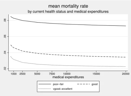
Not surprisingly, the maximum likelihood estimates of the mortality process reveal that better health is associated with lower mortality risk. Combining the mortality and health process estimates, we estimate the effect of medical expenditures on mortality risk. Figure 1 shows the resulting mortality rates by medical spending level and current health status for individuals age 65+. Mortality falls with increased spending, but the effect diminishes as the level of spending increases. The first dollars of medical expenditures are more productive in almost all states, in particular in good health.

4.1.3 Other Institutional Parameters

The resource floor is set at $10, 000. The real rate of return is set at 0.04. We construct co-insurance rates, ψ(), using MEPS data. We take the ratio of out-of-pocket medical expenditures to total medical expenditures as our estimate of the co-insurance rate (see French and Jones, 2011, for a similar methodology). This yields a median co-insurance rate of 25% for individuals with tied-employer insurance, 7% for those receiving government transfers (i.e. those on Medicaid), 100% for those without insurance and ineligible for Medicaid and 20% for those on Medicare. Appendix A provides details on the construction of these shares and the rationale behind other numbers.

4.2 Preference Parameters

The remaining parameters to estimate are θ = (α2, α3, γ, φ1, φ2, σ, β). We estimate these

parameters by the method of simulated moments (MSM) (Gourinchas and Parker, 2002; French, 2005). This is done by matching moments from the data with moments obtained from simulations of the model. The moments chosen are: average wealth over 5-year intervals between ages 35 and 70; average medical expenditures over 5-year intervals between ages 35 and 85; proportion of individuals working, by health status, at 2-year intervals between ages 56 and 68; and finally, mortality rates over 5-year intervals between ages 50 and 95. These profiles are constructed using the methodology outlined in French (2005) and accounting for cohort and family composition effects. Appendix E gives details on the construction of each profile.

The wealth profile primarily provides information on σ and β following the usual iden-tification arguments. The labor force participation moments by health status provide in-formation on γ, φ₁ and φ₂, keeping σ and β constant. Assuming (σ, β) are determined by previous information, the medical expenditures profile helps determining (α₂, α3) given that

the health process is estimated in the first step. We have 50 moments for 7 parameters. The overidentification test statistic therefore has a χ2₅₀₋₇ distribution. More details on the properties of the estimator are found in Appendix E. 10

4.2.1 Estimation Results

Table 1 reports parameter estimates along with standard errors. We obtain an estimate for the general curvature of the utility function, σ = 3.365 (se = 0.958). Given our estimate_b of the consumption share in the utility function, γ = 0.436 (se = 0.005), we obtain the_b coefficient of risk aversion, keeping labor supply fixed, as −(γ(1 −_b bσ) − 1) = 2.03 (French,

10_{Since the baseline utility levels are quite sensitive to the choice of other parameters, we rescale as}

α∗h= −αh

(xγminL 1−γ

)(1−σ)

(1 − σ) , h = 2, 3

Hence, the estimates of α2 and α3 should be interpreted in units of baseline utility measured at xmin and

2005). Hence, our estimate of the coefficient of relative risk aversion is close to estimates reported in the literature, and very close to the estimate of 2 used by Hall and Jones (2007). We estimate that agents are patient, with a discount factor estimate of bβ = 0.984 (se = 0.036). This estimate is slightly lower than the parameter estimate of 0.992 used in Hall and Jones (2007). These parameters are statistically significant at the 1% level. The estimates of the amount of leisure time lost when in poorer health are bφ2 = 371.6

(se = 442.3) and bφ1= 696.1 (se = 708.3), representing 9.2% and 17.4% of maximum leisure

time available. However, these parameter estimates are imprecise and we cannot reject a value of zero. Part of the reason for the imprecision may have to do with the fact that we only model labor force participation and not hours worked. Finally, estimates of α₁ and α2 are respectively 0.190 (se = 0.149) and 0.229 (se = 0.047), with only the latter being

statistically different from zero. Overall, utility increases with health, which has an impact on the desire of agents to invest in health.

4.2.2 Model Fit

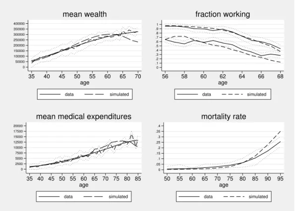
The model fits the data well given that we only have 7 preference parameters and none of these parameters depend on age. The overidentifying restriction test statistic takes a value of 164.8. Formally, the restrictions are rejected (p-value < 0.01). However, inspection of the simulated profiles in Figure 2 shows a relatively close fit. The simulated moments are for the most part within the confidence intervals of the moments estimated from the data. There are three exceptions. First, we predict a decline in wealth after age 65 which we could not detect in the data. One possible explanation is that we did not incorporate bequests in the model (French, 2005). The second exception is labor force participation of individuals in poor health at ages 56 and 58. We over-predict labor force participation at those ages for this group. Two explanations appear plausible. The first is that we did not model disability insurance, which provides another exit route to retirement for individuals in poor health. The other is that we did not model private defined-benefit pensions, which may provide an incentive to stop work early. Despite the fact that we did not allow any of the

preference parameters to depend on health, the model is able to capture the overall patterns of declining labor force participation without any direct dependence of utility on age. The third exception is that we over-predict mortality at advanced ages while under-predicting it at younger ages. However, as we show below the life expectancy estimates implied by the model are roughly consistent with what we observe from mortality data (78.1 years old compared to 77.7). These minor deviations are unlikely to lead to very different simulation results for the scenarios we investigate below.

4.2.3 Income and Insurance Elasticities

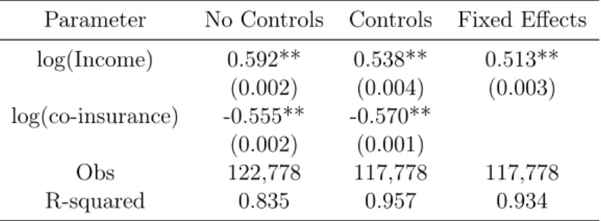
Since the response of medical spending to income and co-insurance rate variation is central to the questions we asked, it is worth investigating the elasticities that the model generates. To do this, we use simulated data generated by the model. We focus on individuals younger than 50 since their labor supply is fixed and, thus, income and co-insurance variation is exogenous, conditional on initial conditions. We perform regression analysis of log spending on the log of the co-insurance rate. The coefficient on log income can be interpreted as an elasticity. We control for age fixed effects. In some specifications, we control for current health and assets. Finally, we also estimate a fixed effects regression. Estimates of the income and co-payment elasticities obtained by regression are reported in Table 2.

The income elasticities range from 0.513 to 0.592. These elasticities fall between macro (closer to 1) and micro (0.2-0.4) estimates of the income elasticity of health spending. Esti-mates are closer to those obtained by Acemoglu et al. (forthcoming). They report a central estimate of 0.7. Hall and Jones (2007) obtain much higher elasticies (higher than 2) as they are able to explain the rise in the fraction of income devoted to health only as a result of income growth. Our model estimates will not lead to a rising share of income devoted to health as income rises.

As for the co-pay elasticity, we obtain regression estimates of -0.555 without controls and -0.570 with controls. This is larger in magnitude than estimates from the RAND Health Insurance Experiment, which are closer to -0.2 (Manning et al., 1987). There are a number

of reasons why we obtain larger elasticities. First, we do not impose a stop-loss on health spending. The RAND Health Insurance Experiment varied co-insurance rates exogeneously in an environment where out-of-pocket expenditures were subject to a limit (Manning et al., 1987). Second, our “random” assignment of insurance status is permanent until age 65 (or until retirement). The assignment of co-insurance rates was limited to a few years in the RAND Health Insurance Experiment. This could explain why our elasticity estimate is larger.

We can also investigate how health spending varies by insurance status near age 65. In Figure 3, we report average simulated total medical expenditures by age and initial insurance status (hence insurance status does not vary for each individual over the period). We see that for those with retiree coverage, there is little jump in medical expenditures at age 65. There is a small increase in spending for those with employer-tied coverage, from $7,253.8 to $8,028.8. This is due to the fact that a fraction of those with employer-tied coverage quit work and hence lose health insurance coverage. The greatest change in medical expenditures at age 65 is found for the uninsured, who spend $3,548.9 on average at age 64 compared to $8,529.6 at age 65. This jump represents an increase of 140% in health spending or a co-pay elasticity (using the effective change in co-pay) of 1.83. Interestingly, there is evidence of intertemporal substitution as medical spending at age 65 is actually higher for the previously uninsured than for those with continued coverage ($8,529.6 vs. $7,488.6). This is consistent with evidence from Card et al. (2008) who find that health care use appears to increase discontinuously at age 65 for those more likely to lack health insurance coverage prior to age 65.

5

Counterfactual Simulations

With the estimates of preferences and technology obtained in section 4, we simulate the ex-perience of a particular cohort under various counterfactual scenarios. We ask the question: how would the 1940 cohort, which was 25 years old in 1965, have fared had changes

affect-ing financial resources, insurance coverage, technology and risk factors not taken place? To answer this question, we look back at some of the important factors that may have changed over the period up to 2005 and that may have affected both health spending and longevity. We roll those factors back to 1965 levels, which we call the 1965 environment. We then successively introduce those changes and evaluate their effect.

5.1 The 1965 compared to the 2005 environment

Changes between 1965 and 2005 can broadly be grouped into four areas of change: financial resources, the generosity of health insurance, technology, and “other” factors.

Financial resources: The income available for consumption and health spending has increased over the years. As in Hall and Jones (2007) we use growth in real per capita GNP, which averaged 2% annually over this period. Affecting after-tax income, taxes were higher in 1965. Gouveia and Strauss (2000) compute average tax rates by income from 1966 to 1989. We use the 1966 tax function instead of the 1989 tax function in our 1965 environment. Finally, the generosity of Social Security benefits has increased over time, primarily due to two effects. First, generosity has increased due to changes in the computation of the primary insurance amount (PIA), which went from replacing 30% to 40% of the ame. Second, the 1983 Social Security reform expanded the delayed retirement credit to 7% for those born in 1940. We eliminate this credit in the 1965 environment.

The generosity of health insurance: After the introduction of Medicare, three key changes have increased the generosity of health insurance in the United States. First, there has been a decline in the uninsured among the non-Medicare population, from 26% in 1962 to 20% in 2005. Second, there has been an expansion of the generosity of employer provided health insurance. We calculate that co-payments decreased from an average of 60% in 1965 to 20% in 2005. Third, changes in Medicare coverage have increased the generosity of benefits. A few years after Medicare’s 1965 introduction, out-of-pocket expenditures were

equal to 30% of the program’s total spending. In 2005, they represented 20% of total outlays according to our calculations.

There are two other sets of factors that may have affected both health and spending: tech-nology and “other factors”. Both are hard to measure from outside sources. Hence, we review the relevant evidence and resort to a calibration exercice.

Technology: Cutler and McClellan (2001) give various examples of important changes in productivity that may have improved survival with overall positive benefits. They point to a 1.5% annual decline in the quality-adjusted price of treating heart attacks as a mea-sure of technological progress. Similarly, Skinner and Staiger (2009) show that in treating heart attacks there is roughly a 3 percentage point difference in survival between hospitals with rapid diffusion of new treatments and those with low diffusion. Improvements in risk adjusted survival average 0.5% year over the period 1985-2004. 11

Other factors: At the same time, other factors have likely affected the health of this cohort. The first obvious candidate is smoking, which has large impacts on mortality. The relevant measure for understanding its effect on life expectancy is the lifetime exposure of a given cohort rather than point-in-time prevalence of smoking (Preston, Glei and Wilmoth, 2011). The former increased until the mid 1980s while the latter declined over the period. Estimates of mortality that can be attributed to smoking range from 10% in 1965 to 24% at peak lifetime exposure in 1985. Preston, Glei and Wilmoth (2011) estimate that life expectancy among men at age 50 would have been 0.9 years higher in 2002 if the increase in lifetime smoking had not taken place. Another key factor is the increased prevalence of obesity, starting in the mid 1970s. Ruhm (2007) uses NHANES data from 1961-62 to 2004 to estimate comparable obesity rates for males and females, using measured rather than self-reported weight and height. For males, obesity rose from 13.4% to 31.5%, or roughly

11_{Medical prices, as measured by the medical CPI, have increased at a rate close to 2% per year. However,}

as discussed in Berndt et al. (2001), this increase in prices likely reflects changes in type and quality of procedures. In this paper, we make the assumption that medical prices, relative to consumption goods, remain constant between 1965 and 2005.

2.1% per year. Both these factors tend to support the view that factors other than financial resources, health insurance and technology may have had an effect on survival rates over the period 1965-2005 - in this case, a negative one. On the positive side, improvements in air pollution may have lead to an independent reduction in mortality rates. One study argues that as much as 15% of the increase in life expectancy in 51 major U.S. cities during the 80s and 90s may be attributed to improvements in air quality (Pope et al., 2009). Hence, it is unclear whether these “other factors” in aggregate had a net positive or negative effect on mortality rates over the period.

We model technology and “other” factors in terms of changes in two parameters of the model. Technological change is modeled as a change in the productivity parameters of the production function δ2,j(see section 3.4). Let κ1be the rate of growth in productivity. Thus,

δ_2,j1965 = e−κ140_δ

2,j. We define the annual rate of growth of mortality due to “other factors”

as κ2. Hence, we have two unknown parameters (κ1, κ2). We use a calibration procedure

to find the value of these parameters. We consider an environment with financial resources and insurance as they were in 1965. Let the simulated average medical expenditures in that scenario with values κ₁ and κ₂ be defined as m_e1965(κ1, κ2). Similarly, simulated life

expectancy is given by _ee1965(κ1, κ2). The actual 1965 values are obtained from National

Health Expenditure Accounts and period life-tables for 1965, m₁₉₆₅ = 569.8 and e1965 =

70.01. We solve for the values of κ1 and κ2 such that we match these values. Relative to

2005, an increase in κ1 tends to lower both health spending and longevity in 1965 while

an increase in κ2 increases longevity while decreasing health spending. The values which

solve this system of two equations are _bκ1 = 0.013 andbκ2= −0.009. Hence, these estimates suggest that negative factors such as the increase in lifetime prevalence of smoking in the first part of the period and the prevalence of obesity outweighed positive factors such as improvements in air quality, and that productivity in health care improved at a pace of 1.3% per year.

5.2 Contributions to Historical Growth in Spending and Longevity We now perform the following counterfactual experiment. Imagine that starting from 1965, we introduce each of the changes separately and look at health spending and longevity. We can then compute the contribution of each factor to the growth of health spending and longevity observed over the period. As we show in section 2, there is the potential for complementarity effects. Hence, the residual growth unexplained by the sum of each contributing factor reflects such effects.

In Table 3, we report the results of the simulations in terms of total medical expenditures, out-of-pocket medical expenditures and life expectancy. We also report as the last outcome a welfare measure based on the comparison of average expected utility at age 25 in each scenario. For scenarios where expected utility is larger than in the 1965 environment, we estimate the fraction of annual consumption in the 2005 environment which would have to be taken away for this average individual to be as well off as in the 1965 environment. Hence, it is a measure of compensating variation (CV).

When letting income grow at 2% per year from the 1965 baseline and implementing tax and Social Security changes, health expenditures increase to $771.7 from $569.1 at the baseline, a 34% increase. The income elasticity is thus 0.29 in the 1965 environment. This suggests that the income elasticity has increased over time since our estimate in the 2005 environment was closer to 0.55 (Table 2). Life expectancy only increases by half a year due to income growth alone. Because the share of income devoted to health care does not rise (it decreases), consumption expenditures increase. This leads to a substantial welfare gain, representing 26.7% of average consumption expenditures in the 2005 environment.

Improvements in insurance from the 1965 baseline do not increase medical expenditures by a much larger amount. With 2005 insurance parameters, average medical expenditures increase to $929.2, a 63% increase. Longevity increases by 0.3 years due to the expansion of insurance. The welfare gains from the expansion of insurance are modest. They represent 3.3% of annual consumption expenditures in the 2005 environment.

in health spending and longevity. Technological change has much larger effects. Allowing for productivity growth in the 1965 environment increases health spending from $569 to $1,972, a 247% increase. The increase in longevity is large, at 9.6 years. Welfare gains, as a result of technology represent close to two thirds of annual consumption in the 2005 environment. We can compare this result to the value of life. Aldy and Viscusi (2004) suggest that $200k is a reasonable estimate for the value of a life year. This suggests that the additional 9.6 years are worth roughly $1.9m. Lifetime consumption (without discounting) is $2.8m in the 2005 environment. Thus $1.9m represent roughly two thirds of life-time utility. Hence, technological change accounts for a large share of the overall welfare gains over the period 1965 to 2005 and our estimates are consistent with a value of a life year close to $200k.

The negative mortality effect of other factors on longevity in 1965 is large (5 years). However, the relevant effect to consider is the comparison between the technology scenario and the 2005 scenario which imposes the trend in these other factors. Longevity is 1.3 years lower in the “other factors” scenario, compared to the technology scenario. This is close to the estimate of Preston, Glei and Wilmoth (2011) who report that male life expectancy would be 0.9 years higher without the trend in smoking.

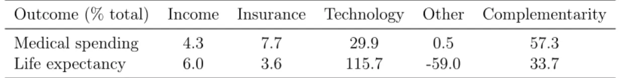
In Table 4, we compute the contribution of each factor to the change in medical spending and life expectancy over the period 1965-2005. Income and insurance together account for less than 12% of the overall increase in medical expenditures. Technology accounts for 30%, while the deterioration of health - probably due to smoking and obesity - accounts for less than 1%. This leaves 57.3% for complementarity effects since by construction allowing for all factors yields 2005 spending level. In other words, the estimates suggest that the observed growth in health care spending would not have occured if these factors had not changed together. A similar story emerges with life expectancy, where most of the observed increase appears to be due to technological change. Other health trends (obesity and smoking) have considerably slowed down the growth of longevity. Interaction effects account for one third of the observed increase in life expectancy.

estimates suggest that the benefits in terms of better health and longevity far outweigh the costs in terms of higher health spending.

5.3 Insurance Coverage and Intertemporal Substitution Effects

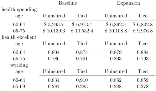
In recent years, proposals to reform health insurance in the U.S. have focused on expanding coverage prior to age 65 and on reforming Medicare to make it sustainable in the future. Expansion of coverage may increase health care spending, health and perhaps even reduce Medicare spending, if uninsured workers currently delay treatment until after they become eligible for Medicare. Our model is well-suited to study such effects as it allows for a response to changes in the price of investing in health along various margins: health care spending, retirement and saving. To gauge the potential for intertemporal substitution, we construct a scenario where we give uninsured workers access to the same insurance plan that workers have. This effectively also provides retiree health coverage to those with tied coverage in the model. We then simulate average health care spending and health status prior to and after Medicare eligibility in that scenario, and compare them to the baseline.

The results, in Table 5, show that medical spending prior to age 65 increases for those without insurance coverage in the baseline (Uninsured). But there is no significant decrease in health spending post age 65 for this group. There is some evidence of intertemporal substitution for those with employer-tied coverage (Tied), but the effects are small. As expected, the fraction working decreases substantially prior to Medicare eligibility for those with tied coverage who do not have a reason to delay retirement anymore (Madrian, 1994). Between ages 60 to 64 the fraction that works decreases from 91% to 86% among those with tied coverage in the baseline. There is evidence of improved health for the uninsured, as the fraction in “very good or excellent health” increases from 80.4% to 87.9% between the ages of 60 and 64. Furthermore, their labor supply increases slightly. However, little of that health gain remains beyond age 65 and health spending is only slightly lower after age 65 for this group. Hence, this simulation suggests that it is unlikely that health spending at older ages will reduce as a result of the provision of insurance coverage to the uninsured prior to

age 65. The changes occur at ages prior to age 65 but little change is observed afterwards.

6

Conclusion

In this paper, we present a life-cycle model of health care spending, savings and retirement in an environment with uncertainty regarding health, earnings and mortality. The model is built on the idea that health is a stock that agents invest in because it provides utility benefits (e.g. it increases the amount of leisure available each year) and because it prolongs life. The model parameters are estimated on data for a representative cohort that lives through a period of rapid health care spending growth. Estimates of preference parameters such as risk aversion and time preference are consistent with existing evidence from savings and retirement models. Other parameter estimates yield very sensible estimates of price and income elasticities of health spending and value of a life year estimates consistent with evidence from the literature. The estimated model enables counterfactual exercises to re-construct the changes experienced over the period 1965 to 2005 and to analyze the effect of potential reforms.

We first considered a set of scenarios aimed at computing the contribution of various factors to growth in health care spending and longevity. We implemented a calibration procedure to estimate the changes in technology and other factors affecting mortality which could rationalize the observed growth. We found, in the parameterization of the health-production function, that improvements in productivity of 1.3% per year, along with an independent deterioration of mortality rates from smoking and obesity at a rate of 0.9% per year, could rationalize the growth observed in income and health insurance generosity over the period.

Starting from 1965, we estimated that each factor independently could not explain the observed growth in health care spending. But, when introduced simultaneously, their mu-tual reinforcement led to rapid growth in health spending. Put simply, growth in income and insurance is not worth much without access to a productive health-production

technol-ogy. According to our estimates, complementarity effects accounted for more than half of the increase observed in medical expenditures over the period. On the longevity side, the estimates suggest that technological progress is the main driver of growth over the period. Together they have produced important welfare benefits that may be worth as much as 76% of 2005 consumption expenditures. As for health-care spending, complementarity effects are also important for explaining the growth in longevity, with an estimated one third coming from that source.

The presence of complementarity effects is perhaps important to understand how rela-tively small differences in income and insurance growth across countries may lead to large aggregate differences in health-spending growth when technological progress is growing at the same pace across countries. Complementarity may strenghten these differences. The U.S. has had both a larger income growth and expansion of health insurance coverage than other developed countries after the Second World War. Even if technological progress has occurred at the same pace across countries, complementarity effects may explain why U.S. health spending growth has outpaced that of other countries, despite health spending being relatively inelastic to income and insurance. If one does not account for complementarities it is difficult to reconcile the observed growth with low income and co-pay elasticities. Fur-thermore, there is much insight to be gained from analyzing within a structural framework whether the growth in medical spending observed over the recent period was “worth it”. Our estimates suggest that the rise of health care spending increased welfare by a great deal, with the largest contribution coming from technological progress.

References

Acemoglu, D., A. Finkelstein, and M. Notowidigdo (forthcoming). “Income and Health Spending: Evidence from Oil Price Shocks” Review of Economics and Statistics MIT Press. Adams, P., M. D. Hurd, D. McFadden, et al. (2003). "Healthy, wealthy, and wise? Tests for direct causal paths between health and socioeconomic status." Journal of Econometrics

112:1, 3-56.

Aldy, J.E. and W. K. Viscusi (2004). "Age Variations in Workers’ Value of Statistical Life," NBER Working Papers 10199, National Bureau of Economic Research, Inc.

Berndt, E., D. Cutler, R. Frank, Z. Griliches, J. Newhouse, J. Triplett (2001). “Price Indexes for Medical Care Goods and Services – An Overview of Measurement Issues”, in Medical Care Output and Productivity, University of Chicago Press

Blau, D.M. and D. Gilleskie, (2008), "The Role of Retiree Health Insurance in the Employ-ment Behavior of Older Men" International Economic Review, 49:2, 475-514.

Card, D., C. Dobkin, and N. Maestas (2008). "The Impact of Nearly Universal Insurance Coverage on Health Care Utilization: Evidence from Medicare." American Economic Review, 98(5): 2242-58.

Currie, J. and B. Madrian (1997). “Health, Health Insurance and the Labor Market”, in Handbook of Labor Economics, eds. O. Ashenfelter and D. Card, Vol 3, Chapter 50, 3309-3416.

Cutler, D. and M. McClellan (2001). “Is Technological Change in Medicine Worth It?” Health Affairs 20:5, 11-29

Cutler, D., A.B. Rosen et S. Vijan (2006a). “The Value of Medical Spending in the United States, 1960–2000”. The New England Journal of Medicine, 355.

Cutler, D., A. Deaton and A. Lleras-Muney (2006b). "The Determinants of Mortality," Journal of Economic Perspectives, 20:3, 97-120.

De Nardi, M., E. French and J. Jones (2010). "Why Do the Elderly Save? The Role of Medical Expenses," Journal of Political Economy, 118:1, 39-75.

French, E. (2005). “The Effects of Health, Wealth, and Wages on Labor Supply and Retire-ment Behavior.” Review of Economic Studies. 72:2, 395-427.

French, E. , J. Jones (2011). "The Effects of Health Insurance and Self-Insurance on Retire-ment Behavior," Econometrica 79:3, 693-732.

Galama, T., A. Kapteyn, R. Fonseca, and P.-C. Michaud (2013). “A Health Production Model with Endogenous Retirement.” Health Economics 22:8, 883-902.

Gerdtham, U.-G. et B. Jonsson (2000). “International Comparisons of Health Expenditures”, Handbook of Health Economics, eds. A. Cuyler et J.-P. Newhouse. 1:1, North-Holland Pub-lishing.

Gourinchas, P.-O. and J.A. Parker (2002). "Consumption Over the Life Cycle," Economet-rica 70:1, 47-89

Gouveia, M. and R. Strauss (2000). “Effective Tax Functions for the U.S. Individual In-come Tax: 1966– 89.” in Proceedings of the 92nd Annual Conference on Taxation, Atlanta, October 24–26. Washington, DC: Nat. Tax Assoc.

Grossman, M. (1972). "On the concept of health capital and the demand for health" Journal of Political Economy 80, 223-255.

Hall, R., and C. Jones (2007). “The Value of Life and the Rise in Health Spending.” The Quarterly Journal of Economics 122:1, 39–72.

Halliday, T.J., He, Hui and Zhang, H. (2009). “Health Investment over the Life Cycle”, IZA DP No. 4482

Hugonnier, J., P. St-Amour and F. Pelgrin (forthcoming): “Health and (other) Asset Hold-ings”, Review of Economic Studies.

Khwaja, A. (2010). "Estimating Willingness to Pay for Medicare Using a Dynamic Life-Cycle Model of Demand for Health Insurance" Journal of Econometrics, 156:1, 130-147.

Madrian, B. (1994), “The Effect of Health Insurance on Retirement”, Brookings Papers on Economic Activity, 25:1, 181-152.

Manning W.G., Newhouse, J. P., Duan, N., Keeler, E., Benjamin, B., Leibowitz, A., Mar-quis, M.S. and Zwanziger, J. (1987), Health Insurance and the Demand for Medical Care: Evidence from a Randomized Experiment. American Economic Review, 77, 251-277. Meara, E. , C. White and D.M. Cutler (2004). "Trends in Medical Spending by Age, 1963-2000," Health Affairs, 176-183.

Murphy, K.M. et R.H. Topel (2006). “The Value of Health and Longevity”. Journal of Po-litical Economy, 114:5, 871-904.

Newhouse, J. (1992). “Medical Care Costs: How Much Welfare Loss?” The Journal of Eco-nomic Perspectives, 6:3, 3-21.

Peltrin, A. and K. Train (2010). "A Control Function Approach to Endogeneity in Consumer Choice Models," Journal of Marketing Research, 47:1, 3-13.

Preston, S. D. Glei, and J. Wilmoth (2011). "Contribution of Smoking to International Differences in Life Expectancy" in International Differences in Mortality at Older Ages: Dimensions and Sources. Washington, DC: The National Academies Press.

Pope, C., M. Ezzati, and D. Dockery (2009). “Fine-Particulate Air Pollution and Life Ex-pectancy in the United States.” New England Journal of Medicine 360:4, 376–386.

Ruhm, C. (2007). “Current and Future Prevalence of Obesity and Severe Obesity in the United States.” Forum for Health Economics & Policy 10:2, 1–28.

Scholz, J.K. and A. Seshadri (2010). Health and Wealth in a Life

Cy-cle Model. Working Paper 224. Michigan Retirement Research Center.

http://ideas.repec.org/p/mrr/papers/wp224.html.

Skinner, J. and D. Staiger (2009). “Technology Diffusion and Productivity Growth in Health Care”, NBER working paper 14865.

Smith, J. (2007). “The Impact of Socioeconomic Status on Health over the Life-Course,” Journal of Human Resources, 42:4, 739-764.

Suen, R. (2005). “Technological Advance and the Growth in Health Care Spending”, Economie d’Avant Garde Research Reports 13.

Tauchen, G. (1986). “Finite State Markov-Chain Approximations to Univariate and Vector Autoregressions.” Economic Letters 20, 177–181.

Yogo, M. (2009). “Portfolio Choice in Retirement: Health Risk and the Demand for Annu-ities, Housing, and Risky Assets” mimeo

Appendix A Institutional Details

Taxes

Taxes are the sum of federal tax, τf(y), the employee portion of the Social Security earnings

tax and the Medicare tax. The federal tax is modeled using the following formula from Gouveia and Strauss (2000):

τf(y) = a0[y − (y−a1 + a2)−1/a1],

where y is the sum of all income sources. We use the 1989 parameters, a₀ = 0.258, a1 = 0.768 and a2 = 0.031. The Social Security earnings tax is 6.2% up to a maximum of

$97,500 in earnings. The Medicare tax is 1.5% of earnings and there is no maximum.

Social Security

The formula for updating the average indexed monthly earnings (AME) prior to age 60 is given by

amet+1= amet+ min(yet, ssmax)/(35 × 12)

where ssmax = 97, 500. After age 60, the formula is given by

amet+1= amet+ (min(yte, ssmax) − χtamet)/(35 × 12)

where χt is the probability that the AME will not be updated (French, 2005). This

proba-bility is computed by simulating earnings histories from the earnings process in the model and counting the frequency of updating using the true ame formula (i.e. the highest 35 years of earnings). This probability is 9.1% at age 60, and it reaches 59% by age 69.

The primary benefit is a piece-wise linear function of ame_t. The bendpoints for someone born in 1940 are $477 and $2,875: each dollar counts for 0.9 below the first bendpoint, for 0.32 in the second segment, and for 0.15 above the second bendpoint.

The full retirement age (FRA) for someone born in 1940 is 65 and 6 months which we round as 65. If the agent claims prior to the FRA, he is penalized with a 6.7% reduction per year. Someone claiming at age 62 will receive 82% of his primary insurance amount (PIA). But if the agent claims after the FRA, he is granted a delayed retirement credit which for someone born in 1940 is 7% per additional year, compounded. Hence, someone claiming at age 70 will receive 40% more. We denote this age adjustment ζ(t). The actuarially fair rate will vary across agents depending on their survival prospects.

At the time of claiming benefits, we adjust the ame_t+1 such that

amet+1 = P IA−1(ζ(t)P IA(amet))

This will permanently set ame_t+1 to a value such that P IA(ame_t+1) = ζ(t)P IA(amet).

Hence, we do not need to keep track of the age when someone claimed, t, in the state space. The agent is allowed to work while collecting benefits. But he will suffer a benefit reduction if his earnings are above a limit, which we set at $10,000 for this cohort. The penalty will depend on age. Prior to the FRA, the penalty is 50%. Hence, each dollar above the earnings limit cuts back current benefits by 50 cents. After the FRA, the penalty is 33%.

Government Transfers

The resource floor is set at $10,000. This figure is derived from the Office of the Assis-tant Secretary for Planning and Evaluation (ASPE, 2008), which states that the maximum monthly benefit payable to a couple with one child under the Temporary Assistance for Needy Families (TANF) program was $495 in 2006. That year, the average monthly benefit of recipients on food stamps (for a 3-person agent) was $283. Hence, prior to age 65, the sum of TANF and food stamp benefits totaled $778/month for a 3-person agent, or $9,336/year (ignoring the lifetime TANF receipt limit). The Social Security Administration reports that the 2004 maximum monthly federal payment for SSI was $552 for a single and $829 for