Bootstrapping Autoregressions with Conditional Heteroskedasticity of Unknown Form

Texte intégral

(1)2003s-17. Bootstrapping Autoregressions with Conditional Heteroskedasticity of Unknown Form Sílvia Gonçalves, Lutz Kilian. Série Scientifique Scientific Series. Montréal Avril 2003. © 2003 Sílvia Gonçalves, Lutz Kilian. Tous droits réservés. All rights reserved. Reproduction partielle permise avec citation du document source, incluant la notice ©. Short sections may be quoted without explicit permission, if full credit, including © notice, is given to the source..

(2) CIRANO Le CIRANO est un organisme sans but lucratif constitué en vertu de la Loi des compagnies du Québec. Le financement de son infrastructure et de ses activités de recherche provient des cotisations de ses organisationsmembres, d’une subvention d’infrastructure du ministère de la Recherche, de la Science et de la Technologie, de même que des subventions et mandats obtenus par ses équipes de recherche. CIRANO is a private non-profit organization incorporated under the Québec Companies Act. Its infrastructure and research activities are funded through fees paid by member organizations, an infrastructure grant from the Ministère de la Recherche, de la Science et de la Technologie, and grants and research mandates obtained by its research teams. Les organisations-partenaires / The Partner Organizations PARTENAIRE MAJEUR . Ministère des Finances, de l’Économie et de la Recherche [MFER] PARTENAIRES . Alcan inc. . Axa Canada . Banque du Canada . Banque Laurentienne du Canada . Banque Nationale du Canada . Banque Royale du Canada . Bell Canada . Bombardier . Bourse de Montréal . Développement des ressources humaines Canada [DRHC] . Fédération des caisses Desjardins du Québec . Gaz Métropolitain . Hydro-Québec . Industrie Canada . Pratt & Whitney Canada Inc. . Raymond Chabot Grant Thornton . Ville de Montréal . École Polytechnique de Montréal . HEC Montréal . Université Concordia . Université de Montréal . Université du Québec à Montréal . Université Laval . Université McGill ASSOCIÉ AU : . Institut de Finance Mathématique de Montréal (IFM2) . Laboratoires universitaires Bell Canada . Réseau de calcul et de modélisation mathématique [RCM2] . Réseau de centres d’excellence MITACS (Les mathématiques des technologies de l’information et des systèmes complexes). Les cahiers de la série scientifique (CS) visent à rendre accessibles des résultats de recherche effectuée au CIRANO afin de susciter échanges et commentaires. Ces cahiers sont écrits dans le style des publications scientifiques. Les idées et les opinions émises sont sous l’unique responsabilité des auteurs et ne représentent pas nécessairement les positions du CIRANO ou de ses partenaires. This paper presents research carried out at CIRANO and aims at encouraging discussion and comment. The observations and viewpoints expressed are the sole responsibility of the authors. They do not necessarily represent positions of CIRANO or its partners.. ISSN 1198-8177.

(3) Bootstrapping Autoregressions with Conditional Heteroskedasticity of Unknown Form* Sílvia Gonçalves†, Lutz Kilian‡ Résumé / Abstract La présence d'hétéroscédasticité conditionnelle est une caractéristique importante de beaucoup de séries temporelles en macroéconomie et en finance. Les méthodes de bootstrap usuelles pour des modèles de régression dynamiques rééchantillonnent les erreurs de façon i.i.d. et ne sont pas valables sous la présence d'hétéroscédasticité conditionnelle. Dans ce papier, nous montrons la validité asymptotique de trois méthodes de bootstrap pour des processus stationnaires autorégressifs dont le terme d'erreur est une différence de martingale. Les méthodes de bootstrap que nous étudions sont le "wild" bootstrap fixé, le "wild" bootstrap récursif et le bootstrap par couples. Une étude de Monte Carlo montre que la performance d'intervalles de confiance basées sur ces méthodes est supérieure à celle des intervalles de confiance basées sur la théorie asymptotique robuste à la présence d'hétéroscédasticité. Par contre, la performance de la méthode de bootstrap usuelle basée sur l'hypothèse i.i.d. des erreurs peut être très mauvaise si les erreurs sont hétéroscédastiques. Nous concluons que les méthodes de bootstrap robustes étudiées dans ce papier doivent remplacer la méthode de bootstrap usuelle dans des applications de bootstrap pour des modèles autorégressifs stationnaires. Mots clés: hétéroscédasticité conditionnelle, wild bootstrap, bootstrap par couples. Conditional heteroskedasticity is an important feature of many macroeconomic and financial time series. Standard residual-based bootstrap procedures for dynamic regression models treat the regression error as i.i.d. These procedures are invalid in the presence of conditional heteroskedasticity. We establish the asymptotic validity of three easy-to-implement alternative bootstrap proposals for stationary autoregressive processes with m.d.s. errors subject to possible conditional heteroskedasticity of unknown form. These proposals are the fixed-design wild bootstrap, the recursive-design wild bootstrap and the pairwise bootstrap. In a simulation study all three procedures tend to be more accurate in small samples than the conventional large-sample approximation based on robust standard errors. In contrast, standard residual-based bootstrap methods for models with i.i.d. errors may be very inaccurate if the i.i.d. assumption is violated. We conclude that in many empirical applications the proposed robust bootstrap procedures should routinely replace conventional bootstrap procedures for autoregressions based on the i.i.d. error assumption. Keywords: Conditional Heteroskedasticity, Wild Bootstrap, Pairwise Bootstrap.. * We thank Javier Hidalgo, Atsushi Inoue, Simone Manganelli, Nour Meddahi, Benoit Perron, Michael Wolf, Jonathan Wright, the associate editor and two anonymous referees for helpful comments. The views expressed in this paper do not necessarily reflect the opinion of the ECB or its staff. † CIREQ, CIRANO and Département de sciences économiques, Université de Montréal. ‡ University of Michigan, European Central Bank and CEPR..

(4) 1. Introduction There is evidence of conditional heteroskedasticity in the residuals of many estimated dynamic regression models in finance and in macroeconomics (see, e.g., Engle 1982; Bollerslev 1986; Weiss 1988). This evidence is particularly strong for regressions involving monthly, weekly and daily data. Standard residual-based bootstrap methods of inference for autoregressions treat the error term as independent and identically distributed (i.i.d.) and are invalidated by conditional heteroskedasticity. In this paper, we analyze two main proposals for dealing with conditional heteroskedasticity of unknown form in autoregressions. The first proposal is very easy to implement and involves an application of the wild bootstrap (WB) to the residuals of the dynamic regression model. The WB method allows for regression errors that follow martingale difference sequences (m.d.s.) with possible conditional heteroskedasticity. We investigate both the fixed-design and the recursive-design implementation of the WB for autoregressions. We prove their first-order asymptotic validity for the autoregressive parameters (and smooth functions thereof) under fairly general conditions including, for example, stationary ARCH, GARCH and stochastic volatility error processes (see, e.g., Bollerslev 1986, Shephard 1996). There are several fundamental differences between this paper and earlier work on the WB in regression models. First, existing theoretical work has largely focused on providing first and second-order theoretical justification for the wild bootstrap in the classical linear regression model (see, e.g., Wu 1986, Liu 1988, Mammen 1993, Davidson and Flachaire 2000). Second, the previous literature has mainly focused on the problem of unconditional heteroskedasticity in cross-sections, whereas we focus on the problem of conditional heteroskedasticity in time series. Third, much of the earlier work has dealt with models restricted under the null hypothesis of a test, whereas we focus on the construction of bootstrap confidence intervals from unrestricted regression models (see Davidson and Flachaire 2000, Godfrey and Orme 2001). The work most closely related to ours is Kreiss (1997). Kreiss established the asymptotic validity of a fixed-design WB for stationary autoregressions with known finite lag order when the error term exhibits a specific form of conditional heteroskedasticity. We provide a generalization of this result to m.d.s. 1.

(5) errors with possible conditional heteroskedasticity of unknown form. Our results cover as special cases the N-GARCH, t-GARCH and asymmetric GARCH models, as well as stochastic volatility models. Kreiss (1997) also proposed a recursive-design WB, under the name of “modified wild bootstrap”, but he did not establish the consistency of this bootstrap proposal for autoregressive processes with conditional heteroskedasticity. We prove the first-order asymptotic validity of the recursive-design WB for finite-order autoregressions with m.d.s. errors subject to possible conditional heteroskedasticity of unknown form. The proof holds under slightly stronger assumptions than the proof for the fixed-design WB. Tentative simulation evidence shows that the recursive-design WB scheme works well in practice for a wide range of models of conditional heteroskedasticity. In contrast, conventional residual-based resampling schemes for autoregressions based on the i.i.d. error assumption may be very inaccurate in the presence of conditional heteroskedasticity. Moreover, the accuracy of the recursive-design WB method is comparable to that of the recursive-design i.i.d. bootstrap when the true errors are i.i.d. The recursive-design WB method is typically more accurate in small samples than the fixed-design WB method. It also tends to be more accurate than the Gaussian large-sample approximation based on robust standard errors. The second proposal for dealing with conditional heteroskedasticity of unknown form involves the pairwise resampling of the observations. This method was originally suggested by Freedman (1981) for cross-sectional models. We establish the asymptotic validity of this method in the autoregressive context and compare its performance to that of the fixed-design and of the recursive-design WB. The pairwise bootstrap is less efficient than the residual-based WB, but - like the fixed-design WB - it remains valid for a broader range of GARCH processes than the recursive-design WB, including EGARCH, AGARCH and GJR-GARCH processes, which have been proposed specifically to capture asymmetric responses to shocks in asset returns (see, e.g., Engle and Ng (1993) for a review). We find in Monte Carlo simulations that the pairwise bootstrap is typically more accurate than the fixed-design WB method, but in small samples tends to be somewhat less accurate than the recursive-design WB when the data are persistent. For large samples these differences vanish, and the pairwise bootstrap is as accurate as. 2.

(6) the recursive-design WB. A third proposal for dealing with conditional heteroskedasticity of unknown form is the resampling of blocks of autoregressive residuals (see, e.g., Berkowitz, Birgean and Kilian 2000). No formal theoretical results exist that would justify such a bootstrap proposal. We do not consider this proposal for two reasons. First, in the context of a well-specified parametric model this proposal involves a loss of efficiency relative to the WB because it allows for serial correlation in the error term in addition to conditional heteroskedasticity. Second, the residual-based block bootstrap requires the choice of an additional tuning parameter in the form of the block size. In practice, results may be sensitive to the choice of block size. Although there are data-dependent rules for block size selection, these procedures are very computationally intensive and little is known about their accuracy in small samples. In contrast, the methods we propose are no more computationally burdensome than the standard residual-based algorithm and very easy to implement. The paper is organized as follows. In section 2 we provide empirical evidence that casts doubt on the use of the i.i.d. error assumption for autoregressions, and we highlight the limitations of existing bootstrap and asymptotic methods of inference when the autoregressive errors are conditionally heteroskedastic. In section 3 we describe the bootstrap algorithms and state our main theoretical results. Details of the proofs are relegated to the appendix. In section 4, we provide some tentative simulation evidence for the small-sample performance of alternative bootstrap proposals. We conclude in section 5.. 2. Evidence Against the Assumption of i.i.d. Errors Standard residual-based bootstrap methods of inference for dynamic regression models treat the error term as i.i.d. The i.i.d. assumption does not follow naturally from economic models. Nevertheless, in many cases it has proved convenient for theoretical purposes to treat the error term of dynamic regression models as i.i.d. This would be of little concern if actual data were well represented by models with i.i.d. errors. Unfortunately, this is not the case in many empirical studies. One approach in applied work has been simply to ignore the problem and to treat the error term as i.i.d. (see, e.g., Goetzmann and Jorion 1993, 1995). An alternative approach has been to impose a parametric model of conditional 3.

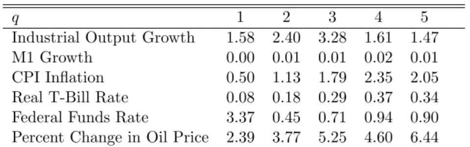
(7) heteroskedasticity. For example, Bollerslev (1986) models inflation as an autoregressive process with GARCH(1,1) errors. Similarly, Hodrick (1992) and Bekaert and Hodrick (2001) postulate a VAR model with conditionally Gaussian GARCH(1,1) errors. This approach is not without risks. First, it is not clear whether the class of GARCH models adequately captures the conditional heteroskedasticity in the data. Second, even when the class of GARCH models is appropriate, in practice, the precise form of the GARCH model will be unknown and different specifications may yield different results (see Wolf 2000). Further difficulties arise in the multivariate case. For multivariate GARCH models it is often difficult to obtain reliable numerical estimates of the GARCH parameters. In response, researchers typically impose ad hoc restrictions on the covariance structure of the model (see, e.g., Bollerslev, Engle and Wooldridge 1988, Bollerslev 1990, Bekaert et. al. 1997) that call into question the theoretical validity of the estimates (see Ledoit, Santa-Clara and Wolf 2001). For these reasons, we argue for a nonparametric treatment of conditional heteroskedasticity in dynamic regression models. Whereas the failure of the i.i.d. assumption is well-documented in empirical finance, it is less well known that many monthly macroeconomic variables also exhibit evidence of conditional heteroskedasticity. In fact, both the ARCH and the GARCH model were originally motivated by macroeconometric applications (see Engle 1982; Bollerslev 1986). The workhorse model of empirical macroeconomics is the linear autoregression. Table 1 illustrates that the errors of monthly autoregressions typically cannot be treated as i.i.d. It shows the results of LM tests of the null of no ARCH in the errors of six univariate monthly autoregressive models (see Engle 1982). The data are the growth rate of U.S. industrial output, M1 growth, CPI inflation, the real 3-month T-Bill rate, the nominal Federal Funds rate and the percent change in the price of oil. The data source is FRED, the sample period 1959.1-2001.8, and the autoregressive lag orders have been selected by the AIC. The LM tests strongly reject the assumption of conditional homoskedasticity for the errors of the AR models. Similar results are obtained for a fixed number of 12 lags or of 24 lags. The evidence of non-i.i.d. errors in Table 1 is important because many methods of inference developed for smooth functions of autoregressive parameters (such as impulse responses) do not allow for conditional heteroskedasticity. For example, standard residual-based bootstrap methods for autoregres-. 4.

(8) sions rely on the i.i.d. error assumption and are invalid in the presence of conditional heteroskedasticity, as we will show in the next section. Similarly, the grid bootstrap of Hansen (1999) is based on the assumption of an autoregression with i.i.d. errors. Likewise, standard asymptotic methods for inference in autoregressions rely if not on the i.i.d. assumption, then on the assumption of conditional homoskedasticity. For example, the closed-form solutions for the asymptotic normal approximation of impulse response distributions proposed by L¨ utkepohl (1990) are based on the assumption of conditional homoskedasticity and hence will be inconsistent in the presence of conditional heteroskedasticity. In this paper we study several easy-to-implement bootstrap methods that allow inference in autoregressions with possible conditional heteroskedasticity of unknown form. Unlike the standard residualbased bootstrap for models with i.i.d. innovations these bootstrap methods remain valid under the much weaker assumption of m.d.s. innovations, and they do not require the researcher to take a stand on the existence or specific form of conditional heteroskedasticity. For expository purposes we focus on univariate autoregressive models. Analogous results for the multivariate case are possible at the cost of additional notation.. 3. Theory Let (Ω, F, P ) be a probability space and {Ft } a sequence of increasing σ-fields of F. The sequence of martingale differences {εt , t ∈ Z} is defined on (Ω, F, P ), where each εt is assumed to be measurable with respect to Ft . We observe a sample of data {y−p+1 , . . . , y0 , y1 , . . . , yn } from the following data generating process (DGP) for the time series yt , φ (L) yt = εt ,. (3.1). where φ (L) = 1 − φ1 L − φ2 L2 − . . . − φp Lp , φp 6= 0, is assumed to have all roots outside the unit ¡ ¢0 circle and the lag order p is finite and known. φ = φ1 , . . . , φp is the parameter of interest, which we estimate by ordinary least squares (OLS) using observations 1 through n: Ã !−1 n n X X −1 0 −1 ˆ φ= n Yt−1 Y n Yt−1 yt , t−1. t=1. t=1. 5.

(9) where Yt−1 = (yt−1 , . . . , yt−p )0 . In this paper we focus on bootstrap confidence intervals for φ that are robust to the presence of conditional heteroskedasticity of unknown form in the innovations {εt }. More specifically, we assume the following condition: Assumption A (i) E (εt |Ft−1 ) = 0, almost surely, where Ft−1 = σ (εt−1 , εt−2 , . . .) is the σ-field generated by {εt−1 , εt−2 , . . .} . ¡ ¢ (ii) E ε2t = σ 2 < ∞. (iii) limn→∞ n−1. Pn. t=1 E. ¡ 2 ¢ εt |Ft−1 = σ 2 > 0 in probability.. ¡ ¢ (iv) τ r,s ≡ σ −4 E ε2t εt−r εt−s is uniformly bounded for all t, r ≥ 1, s ≥ 1; τ r,r > 0 for all r. (v) limn→∞ n−1. Pn. t=1 εt−r εt−s E. ¡ 2 ¢ εt |Ft−1 = σ 4 τ r,s in probability for any r ≥ 1, s ≥ 1.. (vi) E |εt |4r is uniformly bounded, for some r > 1. Assumption A replaces the usual i.i.d. assumption on the errors {εt } by the less restrictive martingale difference sequence assumption. In particular, Assumption A does not impose conditional homoskedasticity on the sequence {εt }, although it requires {εt } to be covariance stationary. Assumption A covers a variety of conditionally heteroskedastic models such as ARCH, GARCH, EGARCH and stochastic volatility models (see, e.g. Deo (2000), who shows that a stronger version of Assumption A is satisfied for stochastic volatility and GARCH models). Assumptions (iv) and (v) restrict the fourth order cumulants of εt . Recently, Kuersteiner (2001) derived the asymptotic distribution of efficient instrumental variables estimators in the context of ARMA models with martingale difference errors that are strictly stationary and ergodic, and that satisfy a summability condition on the fourth order cumulants. His result also applies to the OLS estimator in the AR model as a special case. In Theorem 3.1, we provide an alternative derivation of the asymptotic distribution of the OLS estimator of the AR model under the slightly less restrictive Assumption A. We use Kuersteiner’s (2001) notation to characterize the ¡ ¢0 ˆ Using φ−1 (L) = P∞ ψ Lj , we let bj = ψ , . . . , ψ asymptotic covariance matrix of φ. with j−1 j−p j=0 j 6.

(10) ψ 0 = 1 and ψ j = 0 for j < 0. The coefficients ψ j satisfy the recursion ψ s − φ1 ψ s−1 − . . . − φp ψ s−p = 0 for all s > 0 and ψ 0 = 1. We let ⇒ denote convergence in distribution throughout. Theorem 3.1. Under Assumption A,. ´ √ ³ˆ n φ − φ ⇒ N (0, C), where. C = A−1 BA−1 , A = σ2. ∞ X. bj b0j and B = σ 4. j=1. ∞ X ∞ X. bi b0j τ i,j .. i=1 j=1. ˆ is of the traditional “sandwich” form, where The asymptotic covariance matrix of φ ¡ ¢ ¡ ¢ P P 0 A = E n−1 nt=1 Yt−1 Yt−1 and B = V ar n−1/2 nt=1 Yt−1 εt . Under conditional homoskedasticity, B = σ 2 A. In particular, by application of the law of iterated expectations, we have that τ i,i ≡ ¡ ¢ ¡ ¡ ¢¢ ¡ ¢ σ −4 E ε2t ε2t−i = σ −4 E ε2t−i E ε2t |Ft−1 = σ −4 E ε2t−i σ 2 = 1 for all i = 1, 2, . . . . Similarly, we can ˆ=φ ˆ show that τ i,j = 0 for all i 6= j. Thus, for instance in the AR(1) case, the asymptotic variance of φ 1 ¡ 2 P∞ 2 ¢−2 ¡ 4 P∞ 2 ¢ 2 σ simplifies to C = σ i=0 ψ i = 1 − φ1 . i=0 ψ i The validity of any bootstrap method in the context of autoregressions with conditional heteroskedasticity depends crucially on the ability of the bootstrap to allow consistent estimation of the asymptotic covariance matrix C. The standard residual-based bootstrap method fails to do so by not correctly mimicking the behavior of the fourth order cumulants of εt in the conditionally heteroskedastic case, as we now show. Let ˆε∗t be resampled with replacement from the centered residuals. The standard residual-based bootstrap builds yt∗ recursively from ˆε∗t according to ∗0 ˆ yt∗ = Yt−1 φ + ˆε∗t , t = 1, . . . , n,. ¡ ¢0 ∗ = y∗ , . . . , y∗ where Yt−1 t−p , given appropriate initial conditions. The recursive-design i.i.d. boott−1 ¡ ¢ ¡ ∗ ¢ P P ∗ ˆ ∗0 ∗ ε∗t , = V ar∗ n−1/2 nt=1 Yt−1 Yt−1 and Briid strap analogues of A and B are A∗riid = n−1 nt=1 E ∗ Yt−1 ¡ ¢ ¢2 P ¡ ∗ are (conditionally) respectively. Because ˆε∗t is i.i.d. 0, σ ˆ 2 , where σ ˆ 2 = n−1 nt=1 ˆεt − ˆε , ˆε∗t and Yt−1 independent, and ∗ Briid = n−1. n X. n X ¡ ∗ ¡ ∗ ¢ ¢ ∗ ¡ ∗2 ¢ ∗0 ∗2 ∗0 E ∗ Yt−1 Yt−1 ˆεt = n−1 E ∗ Yt−1 Yt−1 E ˆεt = σ ˆ 2 A∗riid .. t=1. t=1. 7.

(11) ∗−1 ∗ ∗ 2 −1 Thus, the bootstrap analogue of C, Criid ≡ A∗−1 ˆ 2 A∗−1 riid Briid Ariid = σ riid , converges in probability to σ A , ¡ ¢ implying that the limiting distribution of the recursive i.i.d. bootstrap is N 0, σ 2 A−1 . As Theorem 3.1. ˆ without imposing further shows, σ 2 A−1 , however, is not the correct asymptotic covariance matrix of φ conditions, e.g., that εt is conditionally homoskedastic. In the general, conditionally heteroskedastic ¡ ¢ case, B depends on σ 4 τ i,j . The recursive-design i.i.d. bootstrap implies E ∗ ˆε∗t−iˆε∗t−j ˆε∗2 =σ ˆ 4 when t i = j and zero otherwise, and thus implicitly sets τ i,j = 1 for i = j and 0 for i 6= j. Given the failure of the standard-residual based bootstrap, we are interested in establishing the first-order asymptotic validity of three alternative bootstrap methods in this environment. Two of the bootstrap methods we study rely on an application of the wild bootstrap (WB). The WB has been originally developed by Wu (1986), Liu (1988) and Mammen (1993) in the context of static linear regression models with (unconditionally) heteroskedastic errors. We consider both a recursive-design and a fixed-design version of the WB. The third method is a natural generalization of the pairwise bootstrap for linear regression first suggested by Freedman (1981) for cross-sectional data. Recursive-design wild bootstrap The recursive-design WB is a simple modification of the usual recursive-design bootstrap method for autoregressions (see e.g. Bose, 1988) which consists of replacing Efron’s i.i.d. bootstrap by the wild bootstrap when bootstrapping the errors of the AR model. More specifically, the recursive-design WB bootstrap generates a pseudo time series {yt∗ } according to the autoregressive process: ∗0 ˆ yt∗ = Yt−1 φ + ˆε∗t , t = 1, . . . , n,. ˆ (L) yt , and where η is an i.i.d. sequence with mean zero and variance one where ˆε∗t = ˆεt η t , with ˆεt = φ t such that E ∗ |η t |4 ≤ ∆ < ∞. We let yt∗ = 0 for all t ≤ 0. Kreiss (1997) suggested this method in the context of autoregressive models with i.i.d. errors, but did not investigate its theoretical justification in more general models. Here, we will provide conditions for the asymptotic validity of the recursive-design WB proposal for finite-order autoregressive processes with possibly conditionally heteroskedastic errors. Establishing the validity of the recursive-design WB requires a strengthening of Assumption A. Specifically, we need Assumption A0 below in order to ensure convergence of the bootstrap estimator. 8.

(12) of the asymptotic covariance matrix C to its correct limit. In contrast, the fixed-design WB and the pairwise bootstrap to be discussed later are valid under the less restrictive Assumption A. Assumption A0 ¡ ¢ (iv0 ) E ε2t εt−r εt−s = 0 for all r 6= s, for all t, r ≥ 1, s ≥ 1. (vi0 ) E |εt |4r is uniformly bounded for some r ≥ 2 and for all t. Assumption A0 restricts the class of conditionally heteroskedastic autoregressive models in two dimensions. First, Assumption A0 (iv0 ) requires τ r,s = 0 for all r 6= s. Milhøj (1985) shows that this assumption is satisfied for the ARCH(p) model with innovations having a symmetric distribution. Bollerslev(1986) and He and Ter¨asvirta (1999) extend the argument to the GARCH(p, q) case. In addition, Deo (2000) shows that this assumption is satisfied by certain stochastic volatility models. Assumption A0 (iv0 ) excludes some non-symmetric parametric models such as asymmetric EGARCH. Second, we now require the existence of at least eight moments for the martingale difference sequence {εt } as opposed to only 4r moments, for some r > 1, as in Assumption A. A similar moment condition was used by Kreiss (1997) in his Theorem 4.3, which shows the validity of the recursive-design WB for possibly infinite-order AR processes with i.i.d. innovations. The strengthening of Assumption A is crucial to showing the asymptotic validity of the recursivedesign WB in the martingale difference context. In particular, conditional on the data, and given the © ∗ ∗ ∗ª ¡ ¢ independence of {η t }, Yt−1 ˆεt , Ft can be shown to be a vector m.d.s., where Ft∗ = σ η t , η t−1 , . . . , η 1 . P ∗2 ∗ Y ∗0 ˆ ∗ We use Assumption A0 (vi0 ) to ensure convergence of n−1 nt=1 Yt−1 to Brwb ≡ t−1 εt ¢ ¡ P ∗ ˆ V ar∗ n−1/2 nt=1 Yt−1 ε∗t , thus verifying one of the conditions of the CLT for m.d.s. Assumption ∗ to the correct limiting variance A0 (iv0 ) ensures convergence of the recursive-design WB variance Brwb ³ ´0 P Pt−1 ˆ ∗ ∗ ≡ ˆ ˆ ˆ ˆ b ˆ ε with b ≡ ψ , . . . , ψ of n−1/2 nt=1 Yt−1 εt . More specifically, letting Yt−1 j j−1 j−p , ψ 0 = 1 j=1 j t−j. ˆ = 0 for j < 0, it follows by direct evaluation that and ψ j ∗ Brwb = n−1. t−1 t−1 X n X X t=1 j=1 i=1. 9. ¡ ¢ ˆbj ˆb0 E ∗ ˆε∗ ˆε∗ ˆε∗2 , i t−j t−i t.

(13) ¡ ¢ Pn−1 ˆ ˆ0 −1 ∗ where E ∗ ˆε∗t−j ˆε∗t−iˆε∗2 = ˆε2t−iˆε2t for i = j and zero otherwise. We can rewrite Brwb as j=1 bj bj n t Pn ˜ ≡ P∞ bj b0 σ 4 τ jj under Assumption A. Without ε2t ˆε2t−j , which converges in probability to B j t=1+j ˆ j=1 P P∞ 0 Assumption A0 (iv0 ) an asymptotic bias term appears in the estimation of B ≡ σ 4 ∞ i=1 j=1 bi bj τ i,j , P which is equal to −σ 4 i6=j bi b0j τ i,j . Assumption A0 (iv0 ) sets τ i,j equal to zero for i 6= j, and thus ensures that the recursive-design WB consistently estimates B. Theorem 3.2 formally establishes the asymptotic validity of the recursive-design WB for finite-order ˆ ∗ denote the recursive-design WB autoregressions with conditionally heteroskedastic errors. Let φ rwb ¡ −1 Pn ¢ P ∗ n ∗ ∗0 −1 n−1 ∗ ∗ ˆ OLS estimator, i.e., φ rwb = n t=1 Yt−1 Yt−1 t=1 Yt−1 yt . Theorem 3.2. Under Assumption A strengthened by Assumption A0 (iv0 ) and (vi0 ), it follows that ¯ ³√ ³ ∗ ´ ´ ³√ ³ ´ ´¯ P ¯ ˆ ˆ ˆ − φ ≤ x ¯¯ → sup ¯P ∗ n φ n φ 0, rwb − φ ≤ x − P. x∈Rp. where P ∗ denotes the probability measure induced by the recursive-design WB. Fixed-design wild bootstrap The fixed-design WB generates {yt∗ }nt=1 according to the equation 0 ˆ yt∗ = Yt−1 φ + ˆε∗t , t = 1, . . . , n,. (3.2). ˆ (L) yt , and where η is an i.i.d. sequence with mean zero and variance one such where ˆε∗t = ˆεt η t , ˆεt = φ t ¡ ¢ ˆ ∗ = n−1 Pn Yt−1 Y 0 −1 n−1 Pn Yt−1 y ∗ . that E ∗ |η t |2r ≤ ∆ < ∞. The fixed-design WB estimator is φ f wb t t−1 t=1 t=1 The fixed-design WB corresponds to a regression-type bootstrap method in that (3.2) is a fixed-design regression model, conditional on the original sample. The fixed-design WB was suggested by Kreiss (1997). Kreiss’ (1997) Theorem 4.2 proves the first-order asymptotic validity of the fixed-design WB for finite-order autoregressions with conditional heteroskedasticity of a specific form. More specifically, P he postulates a DGP of the form yt = pi=1 φi yt−i + σ (yt−1 ) vt , where vt is i.i.d.(0, 1) with finite fourth moment. The i.i.d. assumption on the rescaled innovations vt is violated if for instance the conditional moments of vt depend on past observations. We prove the first-order asymptotic validity of the fixed-design WB of Kreiss (1997) under a broader set of regularity conditions, namely Assumption A.. 10.

(14) Theorem 3.3. Under Assumption A, ¯ ³√ ³ ∗ ´ ´¯ ´ ´ ³√ ³ P ¯ ˆ ˆ ˆ − φ ≤ x ¯¯ → sup ¯P ∗ n φ n φ 0, f wb − φ ≤ x − P. x∈Rp. where P ∗ denotes the probability measure induced by the fixed-design WB. In contrast to the recursive-design WB, the ability of the fixed-design WB to estimate consisˆ does not require a strengthening of Astently the variance, and hence the limiting distribution, of φ ˆ∗ sumption A. Specifically, the variance of the limiting conditional bootstrap distribution of φ f wb is ¡ −1/2 Pn ¢ Pn ∗−1 ∗ ∗ −1 0 ∗ ∗ given by A∗−1 ε∗t = t=1 Yt−1 Yt−1 and Bf wb ≡ V ar n t=1 Yt−1 ˆ f wb Bf wb Af wb , where Af wb = n P P P 0 ˆ n−1 nt=1 Yt−1 Yt−1 ε2t . Under Assumption A one can show that A∗f wb → A and Bf∗wb → B, thus ensuring P. ∗−1 ∗ −1 −1 ≡ C. that A∗−1 f wb Bf wb Af wb → A BA. Pairwise bootstrap Another bootstrap method that captures the presence of conditional heteroskedasticity in autoregressive models consists of bootstrapping “pairs”, or tuples, of the dependent and the explanatory variables in the autoregression. This method is an extension of Freedman’s (1981) bootstrap method for the correlation model to the autoregressive context. In the AR(p) model, it amounts to resam¡ ¢ 0 pling with replacement from the set of tuples yt , Yt−1 = (yt , yt−1 , . . . , yt−p ), t = 1, . . . , n. Let ©¡ ∗ ∗0 ¢ ¡ ∗ ∗ ¢ ª ∗ yt , Yt−1 = yt , yt−1 , . . . , yt−p , t = 1, . . . , n be an i.i.d. resample from this set. Then the pair¡ ¢ ˆ ∗ = n−1 Pn Y ∗ Y ∗0 −1 n−1 Pn Y ∗ y ∗ . The bootstrap wise bootstrap estimator is defined by φ pb t=1 t−1 t−1 t=1 t−1 t h¡ ¢ i ˆ since φ ˆ is the parameter value that minimizes E ∗ y ∗ − Y ∗0 φ 2 . The following analogue of φ is φ, t t−1 theorem establishes the asymptotic validity of the pairwise bootstrap for the AR(p) process with m.d.s. errors satisfying Assumption A. Theorem 3.4. Under Assumption A, it follows that ¯ ³√ ³ ∗ ´ ´ ³√ ³ ´ ´¯ P ¯ ˆ −φ ˆ ≤x −P ˆ − φ ≤ x ¯¯ → 0, sup ¯P ∗ n φ n φ pb. x∈Rp. where P ∗ denotes the probability measure induced by the pairwise bootstrap.. 11.

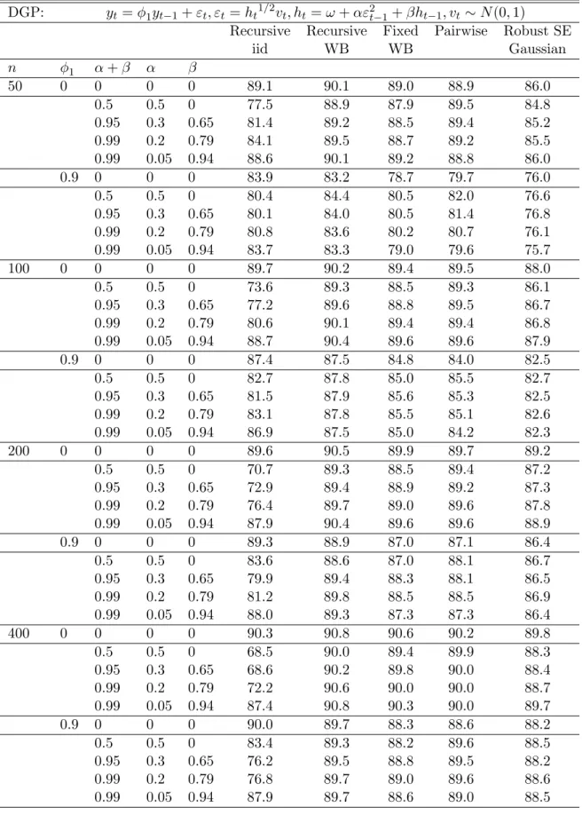
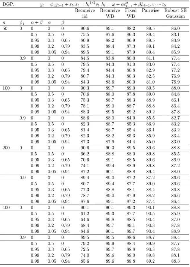
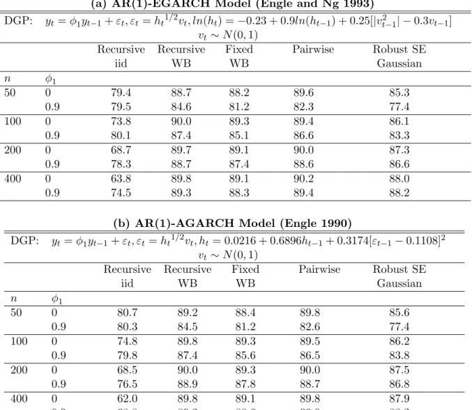
(15) Asymptotic validity of bootstrapping the studentized slope parameter Corollary 3.1 below establishes the asymptotic validity of bootstrapping the t-statistic for the ele∗. ˆ denote the OLS estimator of φ obtained under any of the three ments of φ. To conserve space, we let φ ∗0 ) to denote bootstrap robust bootstrap resampling schemes studied above. Similarly, we use (yt∗ , Yt−1 ∗ =Y data in general. In particular, we implicitly set Yt−1 t−1 for the fixed-design WB. √. For a typical element φj a bootstrap percentile-t confidence interval is based on tφˆ ∗ = j. bootstrap analogue of the t-statistic tφˆ = j. √ ˆ n(φj −φj ) √ . ˆjj C. ∗. ˆ −φ ˆ ) n(φ j qj , ∗ ˆ C. the. jj. In the context of (conditional) heteroskedasticity,. ∗ are the heteroskedasticity-consistent variance estimators evaluated on the original and on Cˆjj and Cˆjj. the bootstrap data, respectively. Specifically, for the bootstrap t-statistic let ˆ ∗ Aˆ∗−1 , with Cˆ ∗ = Aˆ∗−1 B Aˆ∗ = n−1. n X. ∗ ∗0 ˆ ∗ = n−1 Yt−1 Yt−1 and B. t=1. n X. ∗ ∗0 ∗2 Yt−1 Yt−1 e εt ,. t=1. ˆ ∗0 Y ∗ are the bootstrap residuals. where e ε∗t = yt∗ − φ t−1 Corollary 3.1. Assume Assumption A holds. Then, for the fixed-design WB and the pairwise bootstrap, it follows that ¯ ³ ´ ³ ´¯ ¯ ¯ P sup ¯P ∗ tφˆ ∗ ≤ x − P tφˆ ≤ x ¯ → 0, j = 1, . . . , p. x∈R. j. j. If Assumption A is strengthened by Assumption A0 (iv0 ) and (vi0 ), then the above result also holds for the recursive-design WB.. 4. Simulation Evidence In this section, we study the accuracy of the bootstrap approximation proposed in section 3 for sample sizes of interest in applied work. We focus on the AR(1) model as the leading example of an autoregressive process. The DGP is yt = φ1 yt−1 + εt with φ1 ∈ {0, 0.9}. In our simulation study we allow √ for GARCH(1,1) errors of the form εt = ht vt , where vt is i.i.d. N (0, 1) and ht = ω + αε2t−1 + βht−1 , t = 1, . . . , n. We normalize the unconditional variance of εt to one. In addition to conditional N(0,1) innovations we also consider GARCH models with conditional t5 -errors (suitably normalized to have 12.

(16) unit variance). For β = 0 this model reduces to an ARCH(1) model. For α = 0 and β = 0 the error sequence reduces to a sequence of (possibly non-Gaussian) i.i.d errors. We allow for varying degrees of volatility persistence modeled as GARCH processes with α + β ∈ {0, 0.5, 0.95, 0.99}. The parameter settings for α and β are similar to settings found in applied work. In addition, we consider AR(1) models with exponential GARCH errors (EGARCH), asymmetric GARCH errors (AGARCH) and with the GJR-GARCH errors proposed by Glosten, Jaganathan and Runkle (1993). Our parameter settings are based on Engle and Ng (1993). Finally, we also consider the stochastic volatility model εt = vt exp(ht ) with ht = λht−1 + 0.5ut , where |λ| < 1 and (ut , vt ) is a sequence of independent bivariate normal random variables with zero mean and covariance matrix diag(σ 2u , 1). This model is a m.d.s. model and satisfies Assumption A. We follow Deo (2000) in postulating the values (0.936, 0.424) and (0.951, 0.314) for (λ, σ u ). These are values obtained by Shephard (1996) by fitting this stochastic volatility model to real exchange rate data. We generate repeated trials of length n ∈ {50, 100, 200, 400} from these processes and conduct bootstrap inference based on the fitted AR(1) model for each trial. All fitted models include an intercept. For the recursive-design bootstrap methods, we generate the start-up values by randomly drawing observations with replacement from the original data set (see, e.g. Berkowitz and Kilian 2000). The number of Monte Carlo trials is 10,000 with 999 bootstrap replications each. The fixed-design and recursive-design WB involve applying the WB to the residuals of the fitted model. Recall that the WB ˆ −φ ˆ yt−1 , where η is an i.i.d. sequence with mean zero and innovation is ˆε∗t = ˆεt η t , with ˆεt = yt − φ 0 1 t variance one such that E ∗ |η t |4 ≤ ∆ < ∞. In practice, there are several choices for η t that satisfy these conditions. In the baseline simulations we use η t ∼ N (0, 1). Our results are robust to alternative choices, as will be shown at the end of this section. We are interested in studying the coverage accuracy of nominal 90% symmetric percentile-t bootstrap confidence intervals for the slope parameter φ1 . We also considered equal-tailed percentile-t intervals, but found that symmetric percentile-t intervals of the form µ ¶ q q ∗ −1/2 ∗ −1/2 ˆ −t n ˆ +t n φ Cˆ11 , φ Cˆ11 , 1 1 0.9 0.9. 13.

(17) where Pr(|tφˆ ∗ | ≤ t∗0.9 ) = 0.9, virtually always were slightly more accurate. Unlike the percentile interval, 1. the construction of the bootstrap-t interval requires the use of an estimate of the standard error of √ ˆ∗ ˆ n(φ1 − φ1 ). We use the heteroskedasticity-robust estimator of the covariance proposed by Nicholls and Pagan (1983) based on work by Eicker (1963) and White (1980): (X 0 X)−1 X 0 diag(ˆε2t )X(X 0 X)−1 , where X denotes the regressor matrix of the AR model. We also experimented with several modified robust covariance estimators (see MacKinnon and White 1985, Chesher and Jewitt 1987, Davidson and Flachaire 2000). For our sample sizes, none of these estimators performed better than the basic estimator proposed by Nicholls and Pagan (1983). Finally, virtually identical results were obtained based on WB bootstrap standard error estimates. The latter approach involves a nested bootstrap loop and is not recommended for computational reasons. As a benchmark we also include the coverage rates of the Gaussian large-sample approximation based on Nicholls-Pagan robust standard errors. The simulation results are in Tables 2-5. Starting with the results for N-GARCH errors in Table 2, several broad tendencies emerge. First, the accuracy of the standard recursive-design bootstrap procedure based on i.i.d. resampling of the residuals is high when the model errors are truly i.i.d., but can be very poor in the presence of N-GARCH. In the latter case, accuracy tends to deteriorate for large n. Second, for sample sizes of 100 or larger, conventional large-sample approximations based on robust standard errors tend to be more accurate than the recursive-design i.i.d. bootstrap in the presence of N-GARCH, but less accurate for models with i.i.d. errors. In either case, the coverage rates may be substantially below the nominal level. Third, all three robust bootstrap methods tend to be more accurate than the i.i.d. bootstrap or the conventional Gaussian approximation, when the errors are conditionally heteroskedastic. Fourth, for persistent processes, the accuracy of the recursivedesign WB is typically higher than that of the pairwise bootstrap. For large n these differences vanish and both methods are about equally accurate. The accuracy of the recursive-design wild bootstrap is comparable to that of the recursive-design i.i.d. bootstrap for models with i.i.d. errors. The fixed-design WB is typically less accurate than the recursive-design WB and the pairwise bootstrap, although the. 14.

(18) discrepancies diminish for large n. The results for the AR(1) model with t5 -GARCH errors in Table 3 are qualitatively similar, except that the accuracy of the recursive-design i.i.d. bootstrap tends to be even lower than for N-GARCH processes. In Table 4 we explore a number of additional models of conditional heteroskedasticity that have been used primarily to model returns in empirical finance. The results for the stochastic volatility model are qualitatively the same as for N-GARCH and t-GARCH. For the other three models, we find that there is little to choose between the recursive-design WB and the pairwise bootstrap. Their accuracy for small samples and highly persistent data tends to be too low, but consistently higher than that of any alternative method. In all other cases, both methods are highly accurate. Neither the recursive-design i.i.d. bootstrap nor the conventional Gaussian approximation perform well. The high accuracy of the recursive-design WB even for EGARCH, AGARCH and GJR-GARCH error processes is surprising, given its lack of theoretical support for these DGPs. Apparently, the failure of the sufficient conditions for the asymptotic validity of the recursive-design WB method has little effect on its performance in small samples. Fortunately, applications in finance, for which such asymmetric volatility models have been developed, invariably involve large sample sizes, conditions under which pairwise resampling is just as accurate as the recursive-design WB and theoretically justified. We conclude this section with a sensitivity analysis of the effect that the choice of η t has on the performance of the wild bootstrap. To conserve space, we focus on the recursive-design WB only. In the baseline simulations we used η t ∼ N (0, 1). Table 5 shows additional results based on the two- point √ √ √ √ distribution η t = −( 5−1)/2 with probability p = ( 5+1)/(2 5) and η t = ( 5+1)/2 with probability 1 − p, as proposed by Mammen (1993), and the two-point distribution η t = 1 with probability 0.5 and η t = −1 with probability 0.5, as proposed by Liu (1988). The DGPs involve N-GARCH errors as in Table 2. The baseline results for η t ∼ N (0, 1) are also included for comparison. Table 5 shows that the coverage results are remarkably robust to the choice of η t . Moreover, none of the three WB resampling schemes clearly dominates the others. Given the computational costs of the simulation study, we have chosen to focus on a stylized autoregressive model, but have explored a wide range of conditionally heteroskedastic errors. Although. 15.

(19) our simulation results are necessarily tentative, they suggest that the recursive-design WB for autoregressions should replace conventional recursive design i.i.d. bootstrap methods in many applications. The pairwise bootstrap provides a suitable alternative when sample sizes are at least moderately large and the possibility of asymmetric forms of GARCH is a practical concern. Even for moderate sample sizes the accuracy of the pairwise bootstrap is slightly higher than that of the fixed-design bootstrap.. 5. Concluding Remarks The aim of the paper has been to extend the range of applications of autoregressive bootstrap methods in empirical finance and macroeconometrics. We analyzed the theoretical properties of three bootstrap procedures for stationary autoregressions that are robust to conditional heteroskedasticity of unknown form: the fixed-design WB, the recursive-design WB and the pairwise bootstrap. Throughout the paper, we established conditions for the first-order asymptotic validity of these bootstrap procedures. We did not attempt to address the issue of the existence of higher-order asymptotic refinements provided by the bootstrap approximation. Arguments aimed at proving asymptotic refinements require the existence of an Edgeworth expansion for the distribution of the estimator of interest. Establishing the existence of such an Edgeworth expansion is beyond the scope of this paper. Moreover, the quality of the finite-sample approximation provided by analytic Edgeworth expansions often is poor and less accurate than bootstrap approximations. Thus, Edgeworth expansions in general are imperfect guides to the relative accuracy of alternative bootstrap methods (see H¨ardle, Horowitz and Kreiss 2001). Indeed, preliminary simulation evidence indicates that wild bootstrap methods based on two-point distributions that may be expected to yield asymptotic refinements in our context do not perform systematically better than the first-order accurate methods studied in this paper. Nevertheless, we found that the robust bootstrap approximation is typically more accurate in small samples than the usual first-order asymptotic approximation based on robust standard errors. Our simulation results also highlighted the dangers of incorrectly modelling the error term in dynamic regression models as i.i.d. We found that conventional residual-based bootstrap methods may be very inaccurate in the presence of conditional heteroskedasticity. The theoretical and simulation results in this paper suggested that no single bootstrap method for 16.

(20) dealing with conditional heteroskedasticity of unknown form will be optimal in all cases. We concluded that the recursive-design WB is well-suited for applications in empirical macroeconomics. This method performs well, whether the error term of the autoregression is i.i.d. or conditionally heteroskedastic, but it lacks theoretical justification for some forms of asymmetric GARCH that have figured prominently in the literature on high-frequency returns. When the sample size is at least moderately large and asymmetric forms of GARCH are a practical concern, the pairwise bootstrap method provides a suitable alternative. The fixed-design WB has the same theoretical justification as the pairwise bootstrap for parametric models, but appears to be less accurate in practice. There are several interesting extensions of the approach taken in this paper. One possible extension is the development of bootstrap methods for conditionally heteroskedastic stationary autoregressions of possibly infinite order. This extension is the subject of ongoing research. Another useful extension would be to establish the validity of the recursive-design WB for regression parameters in I(1) autoregressions that can be written in terms of zero mean stationary regressors, generalizing recent work by Inoue and Kilian (2002) on I(1) autoregressive models with i.i.d. errors. Yet another useful extension would be to establish the asymptotic validity of robust versions of the grid bootstrap of Hansen (1999). These extensions are nontrivial and left for future research.. 17.

(21) Table 1. Approximate Finite-Sample P-Values of the Engle (1982) LM Test of the No-ARCH(q) Hypothesis (in Percent) for Monthly Autoregressions q Industrial Output Growth M1 Growth CPI Inflation Real T-Bill Rate Federal Funds Rate Percent Change in Oil Price. 1 1.58 0.00 0.50 0.08 3.37 2.39. 2 2.40 0.01 1.13 0.18 0.45 3.77. 3 3.28 0.01 1.79 0.29 0.71 5.25. 4 1.61 0.02 2.35 0.37 0.94 4.60. 5 1.47 0.01 2.05 0.34 0.90 6.44. SOURCE: Based on 20000 bootstrap replications under i.i.d. error null hypothesis. All data have been filtered by a univariate AR model, the lag order of which has been selected by the AIC subject to an upper bound of 12 lags.. 18.

(22) Table 2. Coverage Rates of Nominal 90% Symmetric Percentile-t Intervals for φ1 AR(1)-N-GARCH Model DGP:. n 50. φ1 0. 0.9. 100. 0. 0.9. 200. 0. 0.9. 400. 0. 0.9. yt = φ1 yt−1 + εt , εt = ht 1/2 vt , ht = ω + αε2t−1 + βht−1 , vt ∼ N (0, 1) Recursive Recursive Fixed Pairwise Robust SE iid WB WB Gaussian α+β α β 0 0 0 89.1 90.1 89.0 88.9 86.0 0.5 0.5 0 77.5 88.9 87.9 89.5 84.8 0.95 0.3 0.65 81.4 89.2 88.5 89.4 85.2 0.99 0.2 0.79 84.1 89.5 88.7 89.2 85.5 0.99 0.05 0.94 88.6 90.1 89.2 88.8 86.0 0 0 0 83.9 83.2 78.7 79.7 76.0 0.5 0.5 0 80.4 84.4 80.5 82.0 76.6 0.95 0.3 0.65 80.1 84.0 80.5 81.4 76.8 0.99 0.2 0.79 80.8 83.6 80.2 80.7 76.1 0.99 0.05 0.94 83.7 83.3 79.0 79.6 75.7 0 0 0 89.7 90.2 89.4 89.5 88.0 0.5 0.5 0 73.6 89.3 88.5 89.3 86.1 0.95 0.3 0.65 77.2 89.6 88.8 89.5 86.7 0.99 0.2 0.79 80.6 90.1 89.4 89.4 86.8 0.99 0.05 0.94 88.7 90.4 89.6 89.6 87.9 0 0 0 87.4 87.5 84.8 84.0 82.5 0.5 0.5 0 82.7 87.8 85.0 85.5 82.7 0.95 0.3 0.65 81.5 87.9 85.6 85.3 82.5 0.99 0.2 0.79 83.1 87.8 85.5 85.1 82.6 0.99 0.05 0.94 86.9 87.5 85.0 84.2 82.3 0 0 0 89.6 90.5 89.9 89.7 89.2 0.5 0.5 0 70.7 89.3 88.5 89.4 87.2 0.95 0.3 0.65 72.9 89.4 88.9 89.2 87.3 0.99 0.2 0.79 76.4 89.7 89.0 89.6 87.8 0.99 0.05 0.94 87.9 90.4 89.6 89.6 88.9 0 0 0 89.3 88.9 87.0 87.1 86.4 0.5 0.5 0 83.6 88.6 87.0 88.1 86.7 0.95 0.3 0.65 79.9 89.4 88.3 88.1 86.5 0.99 0.2 0.79 81.2 89.8 88.5 88.5 86.9 0.99 0.05 0.94 88.0 89.3 87.3 87.3 86.4 0 0 0 90.3 90.8 90.6 90.2 89.8 0.5 0.5 0 68.5 90.0 89.4 89.9 88.3 0.95 0.3 0.65 68.6 90.2 89.8 90.0 88.4 0.99 0.2 0.79 72.2 90.6 90.0 90.0 88.7 0.99 0.05 0.94 87.4 90.8 90.3 90.0 89.7 0 0 0 90.0 89.7 88.3 88.6 88.2 0.5 0.5 0 83.4 89.3 88.2 89.6 88.5 0.95 0.3 0.65 76.2 89.5 88.8 89.5 88.2 0.99 0.2 0.79 76.8 89.7 89.0 89.6 88.6 0.99 0.05 0.94 87.9 89.7 88.6 89.0 88.5 19.

(23) Table 3. Coverage Rates of Nominal 90% Symmetric Percentile-t Intervals for φ1 AR(1)-t5 -GARCH Model DGP:. n 50. φ1 0. 0.9. 100. 0. 0.9. 200. 0. 0.9. 400. 0. 0.9. yt = φ1 yt−1 + εt , εt = ht 1/2 vt , ht = ω + αε2t−1 + βht−1 , vt ∼ t5 Recursive Recursive Fixed Pairwise Robust SE iid WB WB Gaussian α+β α β 0 0 0 90.6 89.1 88.2 89.5 86.0 0.5 0.5 0 75.5 87.6 86.3 89.4 83.1 0.95 0.3 0.65 80.9 88.2 86.9 89.5 83.9 0.99 0.2 0.79 83.5 88.4 87.3 89.1 84.2 0.99 0.05 0.94 89.5 89.1 87.9 89.4 85.9 0 0 0 84.5 83.8 80.0 81.1 77.4 0.5 0.5 0 79.5 84.3 81.0 83.0 77.4 0.95 0.3 0.65 79.4 84.4 80.8 82.9 77.2 0.99 0.2 0.79 80.7 84.3 80.3 82.5 76.9 0.99 0.05 0.94 84.3 83.6 80.0 81.0 76.9 0 0 0 90.3 89.7 89.0 89.5 88.0 0.5 0.5 0 70.6 88.0 87.8 89.0 84.8 0.95 0.3 0.65 75.3 88.7 88.3 88.9 86.1 0.99 0.2 0.79 78.1 89.0 88.7 88.8 86.4 0.99 0.05 0.94 88.3 89.5 89.2 89.2 87.8 0 0 0 88.6 88.0 84.0 85.5 82.7 0.5 0.5 0 82.3 88.7 85.3 86.9 83.2 0.95 0.3 0.65 81.4 88.7 85.4 86.1 83.2 0.99 0.2 0.79 82.3 88.2 85.3 85.9 83.4 0.99 0.05 0.94 87.3 87.9 84.4 85.0 83.0 0 0 0 90.6 90.3 89.5 89.6 88.8 0.5 0.5 0 66.2 88.8 88.0 89.8 85.5 0.95 0.3 0.65 70.6 89.1 88.5 89.6 86.9 0.99 0.2 0.79 74.1 89.4 88.9 89.8 87.2 0.99 0.05 0.94 87.2 90.1 88.8 89.4 88.0 0 0 0 89.4 89.0 87.2 87.2 86.6 0.5 0.5 0 80.7 89.4 87.7 89.0 86.6 0.95 0.3 0.65 77.3 88.8 88.1 88.4 86.8 0.99 0.2 0.79 78.7 89.0 87.9 88.2 86.6 0.99 0.05 0.94 87.6 89.1 87.2 87.4 86.4 0 0 0 90.1 90.1 89.3 90.1 88.8 0.5 0.5 0 61.2 89.3 87.7 90.5 85.9 0.95 0.3 0.65 64.6 89.8 88.5 90.4 87.0 0.99 0.2 0.79 68.4 89.7 89.1 90.3 87.8 0.99 0.05 0.94 84.6 90.1 89.7 90.4 88.9 0 0 0 89.5 89.5 88.6 88.7 88.4 0.5 0.5 0 79.2 89.9 88.4 89.9 87.7 0.95 0.3 0.65 72.5 89.7 88.8 90.3 87.8 0.99 0.2 0.79 74.0 89.6 89.0 89.8 88.1 0.99 0.05 0.94 85.6 89.6 88.8 89.2 88.3 20.

(24) Table 4. Coverage Rates of Nominal 90% Symmetric Percentile-t Intervals for φ1 (a) AR(1)-EGARCH Model (Engle and Ng 1993) DGP:. n 50 100 200 400. 2 | − 0.3v yt = φ1 yt−1 + εt , εt = ht 1/2 vt , ln(ht ) = −0.23 + 0.9ln(ht−1 ) + 0.25[|vt−1 t−1 ] vt ∼ N (0, 1) Recursive Recursive Fixed Pairwise Robust SE iid WB WB Gaussian φ1 0 79.4 88.7 88.2 89.6 85.3 0.9 79.5 84.6 81.2 82.3 77.4 0 73.8 90.0 89.3 89.4 86.1 0.9 80.1 87.4 85.1 86.6 83.3 0 68.7 89.7 89.1 90.0 87.3 0.9 78.3 88.7 87.4 88.6 86.6 0 63.8 89.8 89.1 90.2 88.0 0.9 74.5 89.3 88.3 89.4 88.2. (b) AR(1)-AGARCH Model (Engle 1990) DGP:. n 50 100 200 400. yt = φ1 yt−1 + εt , εt = ht 1/2 vt , ht = 0.0216 + 0.6896ht−1 + 0.3174[εt−1 − 0.1108]2 vt ∼ N (0, 1) Recursive Recursive Fixed Pairwise Robust SE iid WB WB Gaussian φ1 0 80.7 89.2 88.4 89.8 85.6 0.9 80.3 84.5 81.2 82.6 77.4 0 74.8 89.8 89.3 89.5 86.2 0.9 79.8 87.4 85.6 86.5 83.8 0 68.5 90.0 89.3 90.0 87.5 0.9 76.5 88.9 87.8 88.7 86.8 0 62.0 89.8 89.1 89.8 87.9 0.9 68.8 89.3 88.6 90.0 88.2. (c) AR(1)-GJR GARCH Model (Glosten, Jaganathan and Runkle 1993) DGP:. n 50 100 200 400. yt = φ1 yt−1 + εt , εt = ht 1/2 vt , ht = 0.005 + 0.7ht−1 + 0.28[|εt−1 | − 0.23εt−1 ]2 vt ∼ N (0, 1) Recursive Recursive Fixed Pairwise Robust SE iid WB WB Gaussian φ1 0 81.8 89.3 88.5 90.0 85.8 0.9 80.0 84.4 81.4 82.3 77.4 0 75.8 90.2 89.6 89.3 86.2 0.9 79.7 87.7 85.4 86.3 83.6 0 70.1 90.2 89.5 89.9 87.8 0.9 77.2 89.0 87.8 89.0 87.0 0 64.1 90.1 89.5 90.2 88.5 0.9 70.5 89.6 88.9 90.2 88.8. 21.

(25) Table 4 (contd.). DGP:. n 50. 100. 200. 400. (d) AR(1)-Stochastic Volatility Model (Shephard 1996) yt = φ1 yt−1 + εt , εt = vt exp(ht ), ht = λht−1 + 0.5ut , (ut , vt ) ∼ N [0, diag(σ 2u , 1)] Recursive Recursive Fixed Pairwise Robust SE iid WB WB Gaussian φ1 λ σu 0 0.936 0.424 82.3 88.0 87.2 89.3 85.8 0.951 0.314 84.9 89.9 87.8 89.4 85.8 0.9 0.936 0.424 80.5 84.4 80.7 83.0 77.4 0.951 0.314 82.0 83.9 80.2 81.8 77.4 0 0.936 0.424 78.2 89.5 88.8 89.7 86.2 0.951 0.314 81.5 89.8 88.9 89.6 86.2 0.9 0.936 0.424 82.0 87.7 85.7 86.3 83.6 0.951 0.314 83.5 87.6 85.1 85.8 83.6 0 0.936 0.424 73.0 89.7 89.0 89.4 87.8 0.951 0.314 78.1 89.7 89.2 89.6 87.4 0.9 0.936 0.424 79.6 89.2 87.5 88.4 87.0 0.951 0.314 82.2 89.0 87.5 88.0 87.0 0 0.936 0.424 69.3 89.8 89.2 90.0 88.5 0.951 0.314 74.7 90.0 89.5 89.6 88.5 0.9 0.936 0.424 76.4 89.7 89.0 89.4 88.8 0.951 0.314 79.9 89.5 88.7 89.2 88.8. 22.

(26) Table 5. Coverage Rates of Nominal 90% Symmetric Percentile-t Intervals for φ1 AR(1)-N-GARCH Model DGP:. n 50. 100. 200. 400. yt = φ1 yt−1 + εt , εt = ht 1/2 vt , ht = ω + αε2t−1 + βht−1 , vt ∼ N (0, 1) Alternative recursive-design WB schemes N(0,1) Mammen Liu φ1 α + β α β 0 0 0 0 90.1 89.2 88.9 0.5 0.5 0 88.9 88.9 88.6 0.95 0.3 0.65 89.2 88.9 88.7 0.99 0.2 0.79 89.5 89.1 88.8 0.99 0.05 0.94 90.1 89.1 88.7 0.9 0 0 0 83.2 83.8 84.3 0.5 0.5 0 84.4 85.2 85.4 0.95 0.3 0.65 84.0 84.0 84.6 0.99 0.2 0.79 83.6 83.7 84.3 0.99 0.05 0.94 83.3 83.7 84.3 0 0 0 0 90.2 90.0 89.4 0.5 0.5 0 89.3 89.3 88.7 0.95 0.3 0.65 89.6 89.4 89.2 0.99 0.2 0.79 90.1 89.4 89.1 0.99 0.05 0.94 90.4 89.8 89.4 0.9 0 0 0 87.5 87.0 87.3 0.5 0.5 0 87.8 87.9 88.1 0.95 0.3 0.65 87.9 87.2 87.6 0.99 0.2 0.79 87.8 87.4 87.9 0.99 0.05 0.94 87.5 87.1 87.4 0 0 0 0 90.5 90.3 89.9 0.5 0.5 0 89.3 89.3 89.0 0.95 0.3 0.65 89.4 89.6 89.2 0.99 0.2 0.79 89.7 89.8 89.4 0.99 0.05 0.94 90.4 90.0 89.6 0.9 0 0 0 88.9 88.9 89.0 0.5 0.5 0 88.6 89.5 89.7 0.95 0.3 0.65 89.4 89.5 89.5 0.99 0.2 0.79 89.8 89.5 89.7 0.99 0.05 0.94 89.3 89.4 89.4 0 0 0 0 90.8 90.4 90.1 0.5 0.5 0 90.0 89.9 89.6 0.95 0.3 0.65 90.2 90.0 89.7 0.99 0.2 0.79 90.6 90.2 89.8 0.99 0.05 0.94 90.8 90.3 90.2 0.9 0 0 0 89.7 90.0 89.7 0.5 0.5 0 89.3 90.2 90.2 0.95 0.3 0.65 89.5 90.0 90.2 0.99 0.2 0.79 89.7 90.1 90.1 0.99 0.05 0.94 89.7 90.0 90.0 23.

(27) A. Appendix Throughout this Appendix, K denotes a generic constant independent of n. We use u.i. to mean P Pn uniformly integrable. Given an m × n matrix A, let kAk = m i=1 j=1 |aij |; for a m × 1 vector a, Pm let |a| = i=1 |ai |. For any n × n matrix A, diag (a11 , . . . , ann ) denotes a diagonal matrix with aii , i = 1, . . . , n in the main diagonal. Similarly, let [aij ]i,j=1,...,n denote a matrix A with typical element aij . P∗. For any bootstrap statistic Tn∗ we write Tn∗ → 0 in probability when limn→∞ P [P ∗ (|Tn∗ | > δ) > δ] = 0 for any δ > 0, i.e. P ∗ (|Tn∗ | > δ) = oP (1). We write Tn∗ ⇒dP ∗ D, in probability, for any distribution D, when weak convergence under the bootstrap probability measure occurs in a set with probability converging to one. The following CLT will be useful in proving results for the bootstrap (cf. White, 1999, p. 133; the Lindeberg condition there has been replaced by the stronger Lyapunov condition here): Theorem A.1 (Martingale Difference Arrays CLT). Let {Znt , Fnt } be a martingale difference ¢ ¡ 2¢ 2 ¡√ P array such that σ 2nt = E Znt , σ nt 6= 0, and define Z¯n ≡ n−1 nt=1 Znt and σ ¯ 2n ≡ V ar nZ¯n = P n−1 nt=1 σ 2nt . If 1. n−1. Pn. 2 σ2 n t=1 Znt /¯. P. − 1 → 0, and. −2(1+δ) −(1+δ) Pn n t=1 E. ¯n 2. limn→∞ σ then. |Znt |2(1+δ) = 0 for some δ > 0,. √ ¯ nZn /¯ σ n ⇒ N (0, 1).. The following Lemma generalizes Kuersteiner’s (2001) Lemma A.1. Kuersteiner’s Assumption A.1 is stronger than our Assumption A in that it assumes that {εt } is strictly stationary and ergodic, and in that it imposes a summability condition on the fourth order cumulants. Lemma A.1. Under Assumption A, for each m ∈ N, m fixed, the vector n−1/2. n X. (εt εt−1 , . . . , εt εt−m )0 ⇒ N (0, Ωm ) ,. t=1. where Ωm = σ 4 [τ r,s ]r,s=1,...,m . Lemmas A.2-A.5 are used to prove the asymptotic validity of the recursive-design WB (cf. Theorem 0. ˆ Yt−1 , and η is i.i.d. (0, 1) such that 3.2). In these lemmas, ˆε∗t = ˆεt η t , t = 1, . . . , n, where ˆεt = yt − φ t E ∗ |η t |4 ≤ ∆ < ∞. Lemma A.2. Under Assumption A, for fixed j ∈ N, 24.

(28) (i) n−1. Pn. (ii) n−1. P∗ ε∗2 t−j → t=j+1 ˆ. σ 2 , in probability;. Pn. P∗ ε∗t−j ˆε∗t → t=j+1 ˆ. 0, in probability.. If we strengthen Assumption A by A0 (vi0 ), then for fixed i, j ∈ N, (iii) n−1. Pn. P∗ ε∗t−j ˆε∗t−iˆε∗2 t → t=max(i,j)+1 ˆ. σ 4 τ i,j 1 (i = j), in probability, where 1 (i = j) is 1 if i = j, and 0. otherwise. The following lemma is the WB analogue of Lemma A.1. Lemma A.3. Under Assumption A strengthened by A(vi0 ), for all fixed m ∈ N, n−1/2. n ³ ´ X ¡ ∗ ∗ ¢0 ˜m , ˆεt ˆεt−1 , . . . , ˆε∗t ˆε∗t−m ⇒dP ∗ N 0, Ω t=m+1. ˜ m ≡ σ 4 diag (τ 1,1 , . . . , τ m,m ) and ⇒dP ∗ denotes weak convergence under the in probability, where Ω bootstrap probability measure. Lemma A.4. Suppose Assumption A holds. Then, n−1 P 0 A ≡ σ2 ∞ j=1 bj bj .. Pn. ∗ ∗ ∗0 P t=1 Yt−1 Yt−1 →. A, in probability, where. Lemma A.5. Suppose Assumption A strengthened by A(vi0 ) holds. Then, n. −1/2. n X. ³ ´ ∗ ˜ , Yt−1 ˆε∗t ⇒dP ∗ N 0, B. t=1. ˜= in probability, where B. P∞. 0 4 j=1 bj bj σ τ j,j .. P A; and (ii) A2n ≡ n−1/2 nt=1 Yt−1 εt © ª P ⇒ N (0, B). First, notice that for any stationary AR(p) process we have yt = ∞ j=0 ψ j εt−j , where ψ j. Proof of Theorem 3.1. We show that (i) A1n ≡ n−1. Pn. P 0 t=1 Yt−1 Yt−1 →. satisfies the recursion ψ s − φ1 ψ s−1 − . . . − φp ψ s−p = 0 with ψ 0 = 1 and ψ j = 0 for j < 0, implying ´0 ³ ¯ ¯ P ¯ψ j ¯ < ∞. We can write Yt−1 = P∞ ψ j εt−1−j , . . . , P∞ ψ j εt−p−j = P∞ bj εt−j with j that ∞ j=0 j=0 j=0 j=1 ¡ ¢0 bj = ψ j−1 , . . . , ψ j−p , where ψ −j = 0 for all j > 0. Hence, by direct evaluation,     ∞ ∞ ∞ ∞ X X X X ¡ ¢ 0 A ≡ E Yt−1 Yt−1 bj b0i εt−j εt−i  = σ 2 bj b0j = σ 2 ψ j ψ j+|k−l|  = E  , j=1 i=1. j=1. j=0. k,l=1,...,p. ¯ ¯ P ¯ ¯ since E (εt−i εt−j ) = 0 for i 6= j under the m.d.s. assumption, and ∞ ψ ψ ¯ j j+|k−l| ¯ ≤ j=0 ¯ Pn P∞ ¯¯ ¯¯ P∞ ¯¯ ¯ 0 m −1 ψ ψ ¯ j+|k−l| ¯ < ∞ for all k, l. To show (i), for fixed m ∈ N, define A1n ≡ n j t=1 Yt−1,m Yt−1,m , j=0 j=0 Pm Pm 0 m P m 2 where Yt−1,m = j=1 bj bj as n → ∞, for j=1 bj εt−j . It suffices to show: (a) A1n → A1 ≡ σ 25.

(29) m each fixed m; (b) Am 1 → A as m → ∞, and (c) limm→∞ lim supn→∞ P [kA1n − A1n k ≥ δ] = 0 for. all δ > 0 (cf. Proposition 6.3.9 of Brockwell and Davis (BD) (1991), p. 207). For (a), we have Pm Pm Pn Pn P 0 −1 −1 Am 1n = j=1 i=1 bj bi n t=1 εt−j εt−i . For fixed i 6= j it follows that n t=1 εt−j εt−i → 0 by Andrews’ (1988) LLN for u.i. L1 -mixingales, since {εt−j εt−i } is a m.d.s. with E |εt−j εt−i |r ≤ kεt−j kr2r kεt−i kr2r < ∆2r < ∞ by Cauchy-Schwartz and Assumption A(vi). For fixed i = j, we can write ³ ´ ³ ´ P P P n−1 nt=1 ε2t−j − σ 2 = n−1 nt=1 zt + n−1 nt=1 E ε2t−j |Ft−j−1 − σ 2 , with zt = ε2t−j − E ε2t−j |Ft−j−1 . Since zt can be shown to be an u.i. m.d.s, the first term goes to zero in probability by Andrews’ LLN. P P The second term also vanishes in probability by Assumption A(iii). Thus, n−1 nt=1 ε2t−j − σ 2 → 0 for Pm P 2 0 m fixed j. It follows that Am 1n → σ j=1 bj bj ≡ A1 , which completes the proof of (a). Part (b) follows °P ° P∞ ° 2 0° ≤ from the dominated convergence theorem, given that ° ∞ b b j=1 j j ° j=1 |bj | < ∞. To prove (c), note that for any δ > 0, P [kA1n − Am 1n k ≥ δ] ≤ ≤. 1 E kA1n − Am 1n k δ     ∞ ∞ n ∞ X X X 2 X |bj |  |bj | n−1 E |εt−i εt−j | ≤  |bj | K → 0 as m → ∞, δ j>m. t=1. j=1. j>m. P since E |εt−i εt−j | ≤ ∆ for some ∆ < ∞, and since ∞ j=1 |bj | < ∞. Next, we prove (ii). We apply P∞ m Proposition 6.3.9 of BD. Let Zt = Yt−1 εt ≡ j=1 bj εt−j εt . For fixed m, define Zt = Yt−1,m εt = Pn Pm m −1/2 t=1 Zt ⇒ N (0, Bm ), with j=1 bj εt−j εt , where Yt−1,m is defined as above. We first show n P Pm 0 4 Bm = m j=1 i=1 bj bi σ τ j,i . We have n. −1/2. n X. Ztm. t=1. =n. −1/2. n X m X. bj εt−j εt =. t=1 j=1. m X j=1. bj n. −1/2. n X t=1. εt−j εt ≡. m X. bj Xnj .. j=1. Pm By Lemma A.1 we have that (Xn1 , . . . , Xnm )0 ⇒ N (0, Ωm ) . Thus, j=1 bj Xnj ⇒ N (0, Bm ), with °P ° P P P∞ ° ° ∞ ∞ ∞ 4 Bm = b0 Ωm b, b0 = (b1 , . . . , bm ) . Since ° j=1 i=1 bj b0i σ 4 τ j,i ° ≤ j=1 i=1 |bj | |bi | σ |τ j,i | < ∞, it P∞ P∞ follows that Bm → B ≡ j=1 i=1 bj b0i σ 4 τ j,i as m → ∞. Finally, for any λ ∈ Rp such that λ0 λ = 1 and for any δ > 0, we have ¯  ¯ ¯ # "¯ ¯ ¯ n X n n ¯ ¯ X X X ¯ ¯ ¯ ¯ λ0 bj εt−j εt ¯¯ ≥ δ  λ0 Zt − n−1/2 λ0 Ztm ¯ ≥ δ = lim lim sup P ¯¯n−1/2 lim lim sup P ¯n−1/2 m→∞ m→∞ ¯ ¯ n→∞ n→∞ ¯ ¯ t=1 j>m t=1 t=1 ¯2  ¯   ¯ ¯X XX ¯ ¯ n X 0 1 ¯  = lim 1  ¯  ≤ lim lim sup λ b ε ε E λ0 bj b0i λσ 4 τ j,i  = 0, j t−j t ¯ ¯ 2 m→∞ m→∞ δ 2 n→∞ nδ ¯ ¯ t=1 j>m j>m i>m where the inequality holds by Chebyshev’s inequality, the second-to-last equality holds by the fact that © ª E (εt−j εt εs−i εs ) = 0 for s 6= t, and all i, j, and the last equality holds by the summability of ψ j and. 26.

(30) the fact that τ j,i are uniformly bounded.¥. P P ∗ ∗ Y ∗0 → Proof of Theorem 3.2. By Lemma A.4, n−1 nt=1 Yt−1 A, in probability, whereas Lemma t−1 ³ ´ P ∗ ˆ ˜ , in probability. Since under Assumption A(iv0 ), B = B, ˜ A.5 implies n−1/2 nt=1 Yt−1 ε∗t ⇒dP ∗ N 0, B the result follows by Polya’s Theorem, given that the normal distribution is everywhere continuous. ¥ P P P 0 Proof of Theorem 3.3. We need to show that (a) n−1 nt=1 Yt−1 Yt−1 → A, and (b) n−1/2 nt=1 Yt−1ˆε∗t ⇒dP ∗ N (0, B) in probability. Part (a) was proved in Theorem 3.1. To show part (b) note that n−1/2. n X. Yt−1ˆε∗t = n−1/2. t=1. = n−1/2. n X t=1 n X. Yt−1 εt η t − n−1/2 Yt−1 εt η t − n−1. t=1. n X. Yt−1 (εt − ˆεt ) η t. t=1 n X. ´ √ ³ 0 ˆ − φ ≡ A∗ − A∗ . Yt−1 Yt−1 ηt n φ 1 2. t=1. ´ P √ ³ˆ P∗ 0 η → n φ − φ = OP (1) and n−1 nt=1 Yt−1 Yt−1 0, in t ¡ ¢ P n 0 η showing that E ∗ n−1 t=1 Yt−1 Yt−1 = 0 and t. P∗. First, note that A∗2 → 0, in probability, since. probability. This follows from ¡ ¢ P Pn P n 0 η −2 0 0 V ar∗ n−1 t=1 Yt−1 Yt−1 t = n t=1 Yt−1 Yt−1 Yt−1 Yt−1 → 0, under Assumption A. We next show ¡ ¢ ¢ ¡ P P 0 ε2 . A∗1 ⇒dP ∗ N (0, B) in probability, where B = V ar n−1/2 nt=1 Yt−1 εt = n−1 nt=1 E Yt−1 Yt−1 t For any λ ∈ Rp , λ0 λ = 1, let Zt∗ = λ0 Yt−1 εt η t . {Zt∗ } is (conditionally) independent such that ¡ ¢ ¡ ¢ P P P 0 ε2 λ. We now apply LyaE ∗ n−1/2 nt=1 Zt∗ = 0 and V ar∗ n−1/2 nt=1 Zt∗ = λ0 n−1 nt=1 Yt−1 Yt−1 t P n 0 0 2 punov’s Theorem (e.g. Durrett, 1995, p.121). Let α∗2 n =λ t=1 Yt−1 Yt−1 εt λ. By arguments similar to P. Theorem 3.1, n−1 α∗2 n → B. If for some r > 1 α∗−2r n. n X. P. E ∗ |Zt∗ |2r → 0. (A.1). t=1. Pn Pn ∗ dP ∗ ∗ dP ∗ N (0, 1) in probability. By Slutsky’s Theorem, it follows that n−1/2 then α∗−1 n t=1 Zt ⇒ t=1 Zt ⇒ ¡ ¢ N 0, λ0 Bλ . To show (A.1), note that the LHS can be written as µ. α∗2 n n. ¶−r n−r. n X ¯ 0 ¯ ¯λ Yt−1 εt ¯2r E ∗ |η t |2r . t=1. ¯ ¯ ¯2r P ¯ ¯ ¯ Thus, it suffices to show that E ¯n−r nt=1 ¯λ0 Yt−1 εt ¯ E ∗ |η t |2r ¯ → 0. Since E ∗ |η t |2r ≤ ∆ < ∞, this ¯ ¯2r holds provided E ¯λ0 Yt−1 εt ¯ ≤ ∆ < ∞, which follows under Assumption A. ¥ ˆ 0 Y ∗ , and ε∗ = y ∗ − φ0 Y ∗ . We show that ˆ 0 Yt−1 , ˆε∗ = y ∗ − φ Proof of Theorem 3.4 Let ˆεt = yt − φ t t t t t−1 t−1 ∗ P P P n n ∗ ∗ d ∗ ∗0 −1/2 −1 ∗ P N (0, B) in probability. We εt ⇒ (i) n t=1 Yt−1 ˆ t=1 Yt−1 Yt−1 → A in probability, and (ii) n can write, n−1. n X t=1. ( ∗ ∗0 Yt−1 Yt−1 −A =. n−1. n X t=1. ∗ ∗0 Yt−1 Yt−1 − n−1. n X t=1. 27. ) 0 Yt−1 Yt−1. ( + n−1. n X t=1. ) 0 Yt−1 Yt−1 −A. ≡ A∗1 + A2 ..