Contents lists available atScienceDirect
Electric Power Systems Research
journal homepage:www.elsevier.com/locate/epsrThe role of power-to-gas and carbon capture technologies in cross-sector
decarbonisation strategies
Mathias Berger
a,*
, David Radu
a, Raphaël Fonteneau
a, Thierry Deschuyteneer
b,
Ghislain Detienne
b, Damien Ernst
aaDepartment of Electrical Engineering and Computer Science, University of Liège, Allée de la Découverte 10, 4000 Liège, Belgium bFluxys, Brussels, Belgium
A R T I C L E I N F O Keywords:
Power-to-gas Gas storage
Integrated energy systems Optimal system planning Hydrogen integration Carbon capture
A B S T R A C T
This paper proposes an optimisation-based framework to tackle long-term centralised planning problems of multi-sector, integrated energy systems including electricity, hydrogen, natural gas, synthetic methane and carbon dioxide. The model selects and sizes the set of power generation, energy conversion and storage as well as carbon capture technologies minimising the cost of supplying energy demand in the form of electricity, hy-drogen, natural gas or synthetic methane across the power, heating, transportation and industry sectors whilst accounting for policy drivers, such as energy independence, carbon dioxide emissions reduction targets, or support schemes. The usefulness of the model is illustrated by a case study evaluating the potential of sector coupling via power-to-gas and carbon capture technologies to achieve deep decarbonisation targets in the Belgian context. Results, on the one hand, indicate that power-to-gas can only play a minor supporting role in cross-sector decarbonisation strategies in Belgium, as electrolysis plants are deployed in moderate quantities whilst methanation plants do not appear in any studied scenario. On the other hand, given the limited renewable potential, post-combustion and direct air carbon capture technologies clearly play an enabling role in any decarbonisation strategy, but may also exacerbate the dependence on fossil fuels.
1. Introduction
The effective integration of energy systems relying on different vectors is envisioned to hold great promise for better integrating re-newable energy sources into energy systems and achieving deep dec-arbonisation objectives[1].
On the one hand, the very large-scale deployment of technologies harnessing renewable energy sources for electricity generation has often lead to large amounts of curtailed electricity[2]and an accrued need for short and long-term storage capacities in the power system to balance volatile as well as seasonal renewable production patterns. As no electrical, electrochemical, thermal or mechanical storage options (besides perhaps hydroelectric reservoirs, including pumped-storage hydroelectricity) currently offer cheap, grid-scale, long-term storage, and given the fact that in some regions, very large-scale gas storage facilities are available for low-cost, long-term storage, power-to-gas technologies have been proposed as a complement to standard power generation and storage technologies[3,4]. On the other hand, in order to significantly reduce carbon dioxide emissions, sectors such as heating, transportation and industry should also be supplied with
low-carbon energy. In this respect, synthetic fuels produced through an integrated power-to-gas chain including electrolysis and methanation processes are also envisioned to play a role[5,6].
Against this backdrop, this paper proposes a framework to tackle long-term centralised planning problems of integrated energy systems coupling four carriers and a commodity, namely electricity, hydrogen, natural gas, methane and carbon dioxide. The capacities of power generation, energy conversion as well as short and long-term storage technologies are sized to minimise the cost of supplying energy de-mands in the form of electricity, hydrogen, and natural gas across the power, heating, transportation and industry sectors. Policy drivers such as energy security and independence, carbon dioxide emission quotas and support schemes for selected technologies are also accounted for. Moreover, a wide range of technological options is considered, in-cluding solar photovoltaic panels, on/offshore wind turbines, open and combined-cycle gas turbines, combined heat and power, waste, biomass and nuclear power plants, electrolysis, methanation, steam methane reforming, direct air and post-combustion carbon capture units, as well as battery, pumped-hydro, carbon dioxide, hydrogen and natural gas storage.
https://doi.org/10.1016/j.epsr.2019.106039
Received 1 May 2019; Received in revised form 3 August 2019; Accepted 18 September 2019 ⁎Corresponding author.
E-mail address:mathias.berger@uliege.be(M. Berger).
Electric Power Systems Research 180 (2020) 106039
Available online 09 January 2020
0378-7796/ © 2019 Elsevier B.V. All rights reserved.
Nomenclature
Abbreviations
B battery storage BM biomass power plant CAPEX capital expenditure CCGT combined-cycle gas turbine
CH4 methane
CHP combined heat and power plant CNG compressed natural gas CO2 carbon dioxide CO2eq CO2-equivalent
DAC direct air (carbon) capture E electricity
EL electrolysis plant ENS energy not served EV electric vehicle
FOM fixed operation and maintenance GW(h) gigawatt(hour)
H2 hydrogen
H2O water
kt kilotonne
kt/h kilotonne/hour LNG liquified natural gas LP linear program M€ million € MT methanation plant NG natural gas NK nuclear power plant OCGT open-cycle gas turbine
O2 oxygen
PCCC post-combustion carbon capture PH pumped-hydro storage
RES renewable energy sources PV photovoltaic (panels) SMR steam methane reformer TSO transmission system operator VOM variable operation and maintenance VRE variable renewable energy
Won onshore wind (turbines) Woff offshore wind (turbines) WS waste power plant Sets and indices
E set of technologies consuming electricity NG set of technologies consuming natural gas H2 set of technologies consuming hydrogen CO2 set of technologies consuming carbon dioxide d index of days in optimisation horizon e energy carrier index
set of energy carriers with balance equation, i.e., = {E, NG, H }2
p power generation or energy conversion technology (or plant) index
set of power generation and energy conversion technolo-gies
D set of dispatchable power generation technologies running
on exogenous fuels
E set of technologies producing carbon-free electricity E
N set of technologies producing electricity and emitting
carbon dioxide
CO2 set of technologies emitting carbon dioxide that may be equipped with a post-combustion capture unit
H2 set of technologies producing hydrogen
R set of renewable-based power generation technologies
s storage technology (or plant) index set of energy storage technologies
E set of electricity storage technologies
NG set of natural gas storage technologies H2 set of hydrogen storage technologies CO2 set of carbon dioxide storage technologies
t time index
set of time periods
D set of first time periods of every day in optimisation
hor-izon Parameters
βp maximum capture rate of post-combustion carbon capture process for technology p CO2[–]
χs duration ratio of storage technologys [–]
p decremental ramp rate of technology p
D[GW/h] +p incremental ramp rate of technology p D[GW/h]
δt discretisation time step [h]
ηp conversion efficiency of technology p \{PCCC, DAC} ηs self-discharge rate of storage technologys [–] ηs,C charge efficiency of storage technologys [–] ηs,D discharge efficiency of storage technologys [–]
p
0 pre-installed (power) capacity of technology
p R D [GWh/h]
e tIE, maximum exchange capacity for any carrier e {CO }2 [GWh/h] or [kt/h]
p
max maximum capacity of technology p Rthat may be
in-stalled [GWh/h]
λe,t exogenous demand for carriere at t [GWh/h]
E dTR, daily electricity demand from electric vehicles [GWh] μp minimum output power level of technologyp [–] νp specific CO2 emissions of fuel on which technology
p CO2runs [kt/GWh]
νNG specific CO2emissions of natural gas [kt/GWh]
tp normalised production profile value for technology p R
at time t [–]
ϕp,CC electrical energy required per unit mass of CO2captured via PCCC for technology p CO2[GWh/kt]
EDAC electrical energy required per unit mass of CO2captured via DAC [GWh/kt]
NGDAC natural gas energy required per unit mass of CO2captured via DAC [GWh/kt]
ϕSMR electrical energy required per unit energy of H2produced via SMR [–]
Πc molar mass of carrier/commodity c ∈ {CH4, CO2, H2, H2O, O2, CO2} [g/mol]
CO2 CO2emissions quota [kt]
Ψe import budget for carriere [GWh]
CO /CH2 4 ratio of stoichiometric coefficients of CO2and CH4in the methanation reaction [–]
H O/H2 2 ratio of stoichiometric coefficients of H2O and H2in the water electrolysis reaction [–]
O /H2 2 ratio of stoichiometric coefficients of O2 and H2 in the water electrolysis reaction [–]
σs minimum state of charge of storage technologys [–]
s
0 pre-installed energy capacity of storage technologys [GWh]
s
max maximum energy capacity of storage technology s [GWh]
τ number of time periods in a day CO2 specific cost of CO2emissions [M€/kt]
e tIE, economic value of carrier/commodity e {CO }2 at time t [M€/GWh]
The problem is formulated as a linear program (LP) assuming per-fect foresight over the optimisation horizon and perper-fect competition, with high degrees of temporal and techno-economic detail to accurately represent power system operation under high renewable penetration [7]. Investment decisions are made at the initial time instant and no discounting of future money flows is performed. Moreover, an optimi-sation horizon of five years with investment costs reduced to five-year equivalents is used to approximate the problem over the full planning horizon of 20 years, thus reducing the computational burden. The planning and operational problems are solved concurrently, thereby yielding optimal sizes and operational schedules for all technologies. Finally, the framework is applied to the Belgian energy system in order to explore future configurations leading to substantial carbon dioxide emission reductions across sectors.
The remainder of this paper is organised as follows. Section2 re-views related works on the operation and planning of integrated energy systems, and highlights the areas to which the present paper con-tributes. Section 3describes the proposed optimisation formulation, and a case study exploring future configurations of the Belgian energy system is presented in Section4. Finally, Section5concludes the paper and future work avenues are discussed.
2. Related works
The topic of integrated energy systems has recently received con-siderable attention in the academic literature[10]. Early contributions include Bakken and Holen[11], Geidl and Andersson [12]and Man-carella and Chicco [13], which focus on planning, operational and economic aspects of integrated energy systems, respectively. These themes have since developed into key areas of integrated energy sys-tems research. In this section, relevant studies considering the opera-tion of integrated energy systems are briefly reviewed before planning problems and models of interest are discussed.
The operational challenges and opportunities arising from the coupling of the electricity and natural gas systems have been the focus of several papers[3,14–25]. More precisely, the coupling of electricity and gas systems via gas-fired power plants has been investigated in [14–20,24,25], which consider the impact of scheduling strategies and carrier physics on the reliability and performance of coupled systems. Furthermore, the effect of system coupling via power-to-gas technolo-gies on system operation has been analysed by Belderbos[3], Clegg and Mancarella[21], Qadrdan et al.[22]and Li et al.[23]. The operational implications of shifting some of the heat demand from gas to electricity for both networks have also been studied by Qadrdan et al.[26].
Although studying the operation of integrated energy systems
eENS value of lost load for carriere [M€/GWh] fp FOM cost for technologyp [M€/GWh/h] fs K, power-related FOM for technologys [M€/GWh/h] fs S, energy-related FOM for technologys [M€/GWh]
p
fuel fuel cost of technology p D[M€/GWh] p
SS incentive given for producing one unit of energy with technologyp (support scheme) [M€/GWh]
vp VOM cost of technologyp [M€/GWh]
CH4 higher heating value of CH4[GWh/kt] H2 higher heating value of H2[GWh/kt] ζp CAPEX of technologyp [M€/GWh/h]
ζs,K power capacity CAPEX of storage technology s [M €/GWh/h]
ζs,S energy capacity CAPEX of storage technologys [M €/GWh]
Variables
CeIE net economic value resulting from trade of
carrier/com-modity e {CO }2 [M€]
CeENS total cost of energy not served for carriere [M€]
Cp
fuel total fuel cost for technologyp D[M€]
Cp total cost for technologyp , incl. CAPEX, FOM, VOM and excl. fuel cost and carbon tax [M€]
Cp
SS revenue from support scheme for technologyp [M€] Ee ts, state of charge of storage technologys , in the form of
carrier e {CO }2, at time t [kt] Kp
CO,CC2 capacity of post-combustion carbon capture unit equip-ping technology p CO2[kt/h]
KEp capacity of power generation technology p
E EN
[GWh/h]
KEEL capacity of electrolysis plants (electrical side) [GWh/h]
Ks power capacity of storage technologys [GWh/h] KCODAC2 capacity of direct air capture units [kt/h]
KHSMR2 capacity of steam methane reforming plants (hydrogen output) [GWh/h]
KCHMT4 capacity of methanation plants (methane output) [GWh/ h]
Le tENS, energy not served for carriere at time t [GWh/h] LE tTR, electricity demand for EVs at time t [GWh/h]
PCH ,MT4t CH4output of methanation units at time t [GWh/h]
PE tp
, electricity production/consumption of technology
p E EN E {SMR} Eat time t [GWh/h]
PE tp N,, net electricity production/consumption of technology p EN {SMR}at time t [GWh/h]
Pe tIE, net exchange flow of carriere at time t [GWh/h] Pe tI
, imports of carriere at time t [GWh/h] Pe tE, exports of carriere at time t [GWh/h] Pp t
H ,2 hydrogen production/consumption of technology p H2 H2 H2at time t [GWh/h]
PNG,p t natural gas consumption of technology p NG at time
t [GWh/h]
Pe ts C
,, charge flow of carriere in storage technologys , at time t [GWh/h]
Pe ts D,, discharge flow of carrier e in storage technology s , at time t [GWh/h]
Pe ts, net flow of carriere in storage technologys at time t [GWh/h]
Qp t
CO ,2 CO2mass flow produced by technology p CO2at time t [kt/h]
QCO ,c A,2t fraction of CO2mass flow of technology p CO2released into atmosphere at time t [kt/h]
QCO ,c,CC2t fraction of CO2mass flow of technology p CO2captured via PCCC at time t [kt/h]
QCO ,DAC2t CO2mass flow exiting DAC units at time t [kt/h]
QCO ,DAC,2tA CO2mass flow captured from atmosphere via DAC at time
t [kt/h]
QCO ,I 2t CO2mass flow imports at time t [kt/h]
QCO ,E2t CO2mass flow exports at time t [kt/h]
QCO ,IE2t net CO2mass flow exchange at time t [kt/h]
QCO ,MT2t mass inflow of CO2required by methanation plants at time
t [kt/h]
QCO ,s 2t net CO2 mass flow from storage technology s CO2at time t [kt/h]
QH O,EL2 t mass inflow of H2O into electrolysis plants at time t
[kt/h]
QO ,EL2t mass outflow of O2from electrolysis plants at time t
[kt/h]
provides a better understanding of opportunities and challenges stem-ming from the integration of different carriers, it falls short of in-dicating how key system components, especially energy transmission, conversion and storage technologies, should be designed to realise the full potential of system integration. Hence, such analyses must be complemented with (long-term) planning studies, which are reviewed next.
Building upon the energy hub concept introduced by Geidl et al. [12], the same authors propose a framework to tackle integrated energy hub operation and layout problems including storage elements [27]. Though suitable for power generation, energy conversion and storage technology selection, the method does not identify optimal sizes for the selected technologies and relies on a nonlinear, nonconvex optimisation problem, thus proving impractical for long planning horizons. In[28], the authors investigate the deployment of batteries, power-to-gas (producing synthetic methane directly) and seasonal storage to com-plement standard dispatchable and renewable-based power generation technologies, but model details are not given. An updated model, based on a LP formulation and including hydrogen and carbon dioxide car-riers, is presented in [3] but only considers the power sector and a yearly planning horizon. An explicit treatment of the long-term storage problem is made by Gabrielli et al.[29], where a methodology is in-troduced to reduce the computational burden of planning problems including such technologies, handled via a mixed-integer linear pro-gramming formulation. A yearly optimisation horizon is considered, which limits design robustness with respect to yearly weather varia-tions. In[16,30–35], variations on the joint expansion planning pro-blem of electricity and gas systems are tackled, for instance including random outages and uncertain electricity load forecasts [30], en-dogenous nodal gas price formation mechanisms[16], uncertain active and reactive power demands in electricity distribution systems[32], the possibility to build electricity storage[34]or power-to-gas as well as reliability criteria [35]. Such problems are computationally challen-ging, and the temporal resolution used is generally low. The compu-tational complexity is further reduced by the use of convex relaxations [16], a low spatial resolution [31] and decomposition methods [30,32–35]. Despite providing highly valuable insight into how the operation of integrated energy systems influences their design, and partly owing to computational limitations, these studies do not consider the sizing of renewable-based power generation technologies, focus on two carriers and sectors only, and generally fail to assess the environ-mental merits of the resulting system designs, e.g., in terms of carbon dioxide emissions reductions. Finally, Pleßmann et al.[4], Brown et al. [6], Brown and Hörsch[36], Dominkovic et al.[37]have investigated the energy and technology mix which would be needed to achieve deep decarbonisation goals in different regions. In particular, in [4] the amount of energy storage in the form of battery, high-temperature thermal and gas (methane) storage that would be required to power the global electricity demand with 100% renewable energy is assessed. A LP formulation is invoked but not presented, which makes results in-terpretation difficult. In[6]and[36], Brown et al. provide a compre-hensive power system planning model including hydrogen and syn-thetic methane energy carriers and also considering the transportation and heating sectors. The model is spatially and temporally resolved and also includes policy constraints in the form of a carbon dioxide emis-sions budget. However, an optimisation horizon of a single year and a restricted set of technologies are considered, whilst the industry sector is not accounted for. In[37], the energy system design which would lead to a zero carbon system in Southeast Europe is studied via the ENERGYPLAN model. The latter is not spatially resolved, while the optimisation horizon spans a single year.
In summary, building upon our previous work[8], this paper adds to the literature on the planning of integrated energy systems (i) by providing a detailed, highly interpretable and computationally efficient long-term, multi-sector, integrated energy system model along with an open-source Python implementation and comprehensive data resources
[9], (ii) by reporting on a case study focussing on a realistic energy system and quantifying the extent to which power-to-gas technologies and sector coupling may help achieve deep decarbonisation goals.
3. Problem statement and formulation
In this section, the planning problem is stated, the scope of the model is described along with a set of modelling assumptions, and a mathematical formulation is proposed.
3.1. Problem statement
This paper focuses on the long-term planning of multi-sector, in-tegrated energy systems featuring power generation, energy conversion and storage assets, with a view to identify cost-optimal energy system configurations capable of supplying energy demand across sectors in the form of different energy vectors whilst satisfying a set of pre-spe-cified technical and regulatory constraints, e.g. adequacy, reliability or environmental performance targets.
In its full complexity, this problem involves (i) all major existing and promising energy vectors, (ii) all sectors of the economy, (iii) a detailed spatial representation of the underlying energy systems, (iv) a multi-scale time horizon combining long-term, discrete investment decisions with short-term operational ones, (v) an accurate description of the physics and control systems of the underlying carrier networks, (vi) an accurate representation of generation, conversion and storage technologies down to the level of individual plants, (vii) short- and long-run uncertainty.
From a practical perspective, considering all aforementioned fea-tures simultaneously results in an intractable model. Hence, choices must be made depending on the scope and intended use of the model, as discussed next.
3.2. Model scope
In this paper, the emphasis is put on formulating a high-level multi-sector, integrated energy system model with high interpretability and very good tractability. More precisely, a model is sought that allows to quickly evaluate how technology options, policy choices, cost or tech-nical performance assumptions impact energy system design and en-ergy carrier flow patterns. As this paper focusses particularly on the role and integration of RES, power-to-gas, carbon capture and storage (also seasonal storage) technologies, key model attributes include a multi-year planning horizon with high temporal resolution, a high level of techno-economic detail and a wide range of technology options, car-riers and sectors. Key simplifying assumptions are reviewed next. 3.3. Modelling assumptions
Centralised Planning. Investment decisions are made by a central planner, who also operates the energy system, and whose goal is to minimise the cost of supplying energy demand across sectors in the form of various energy vectors.
Investment & operational decisions. A single, multi-year investment horizon is considered. Investment decisions are made at the beginning of the time horizon and assets are immediately available. Operational decisions are made at hourly or sub-hourly time steps of the investment horizon. The investment and operational problems are solved simulta-neously.
Spatial aggregation. The energy system is represented by a single node, and the physics of energy carrier networks is reduced to a single nodal balance equation.
Perfect foresight & knowledge. The central planner has perfect fore-sight and knowledge, that is, future weather and load patterns, as well as all technical and economic parameters are known with certainty. In other words, no uncertainty of any nature is considered.
Linearity of technology models. All technologies and individual plants are represented via linear input-output mathematical models, i.e., conversion and storage processes are described in energy terms, and the inherently nonlinear and nonconvex relationships representing these processes are replaced by linear approximations. Input or output dy-namics are considered for some technologies, but only storage tech-nologies have a simple state space representation. Given the multi-year time horizon, high temporal resolution, high number of technological options and carriers considered, directly introducing nonlinear or nonconvex technology models would greatly complicate and slow the solution procedure, or make the problem intractable altogether. 3.4. Model formulation
3.4.1. Technologies
In the sequel, for the sake of clarity, technology models are pre-sented in a generic fashion. Depending on the application, they may be used to describe individual plants or technology classes, and in-stantiated accordingly. It is worth emphasising that no assumption pertaining to the aggregation of individual plants into technology classes is made nor required to formulate the model.
Noncontrollable renewable technologies. A set R={PV,Won,Woff}of noncontrollable, renewable-based power generation technologies is considered, including solar PV, onshore and offshore wind turbines. The constraints describing the operation and sizing of these technologies can be expressed as
+
PE tp, tp( 0p KEp), t , p R, (1)
KEp maxp , p R, (2)
while investment and operating costs write as
= + + Cp ( p )K P t, p . fp Ep t vp E tp, R (3) Eq.(1)describes the power generation from RES plants and their sizing, where an inequality has been used to allow for curtailment. Eq.(2) expresses the fact that the renewable potential is finite within the boundaries of the system considered. Eq. (3) gives the basic cost structure for investing in and operating technologies harnessing RES, including capital expenditure (CAPEX), fixed operation and main-tenance (FOM) and variable operation and mainmain-tenance (VOM) costs. FOM costs represent the capacity-based share of operating costs, whereas VOM costs represent the fraction of operating costs dependent upon the amount of power produced. This structure is applicable to most technologies discussed in this paper, and exclude fuel costs and CO2emission levies. Finally, it is worth mentioning that curtailment is not penalised, as curtailed production has already been indirectly paid for through investment and operating expenses, and it would otherwise provide an artificial incentive to build technologies reducing it.
Dispatchable technologies with exogenous fuels. A set = {BM, WS, NK}
D of dispatchable power generation technologies
re-lying on exogenous fuels to produce electricity is considered, com-prising biomass, waste, and nuclear power plants. Constraints de-scribing the operation and sizing of these technologies, t , write as + PE tp p K , p , Ep D , 0 (4) + + PE tp P ( K ), p , E tp p p Ep D , , 1 0 (5) + PE tp P ( K ), p , E tp p p Ep D , , 1 0 (6) + µp( p K ) P , p , Ep E tp D 0 , (7) = Qp t P , p {BM, WS}, p E tp p CO ,2 , (8)
whereas costs can be expressed as
= Cp P t, p , t p E tp p D fuel fuel , (9) = Cp Q t, p {BM, WS}. t t p CO2 CO2 CO ,2 (10) Eq.(4)describes the sizing of dispatchable power generation technol-ogies running on exogenous fuels. The sizing variable is the output electrical power. Eqs.(5)and(6)describe ramping constraints (up and down, respectively) on the electrical power output. Eq.(7) enforces must-run constraints for selected technologies. Eq.(8)gives the carbon dioxide mass flow generated by the operation of biomass and waste power plants. Eqs.(9)and(10)provide an expression for fuel costs and costs incurred by technologies emitting carbon dioxide, e.g., as a result of the implementation of a carbon tax or an emissions trading scheme. The remainder of the costs can be expressed via Eq.(3).
Exchanges of carriers and commodities. Both imports and exports of carriers and commodities are envisaged. Let = {E, NG, H }2. Then, the equations describing the exchange of carriers and commodities, t , write as = Pe tIE, Pe tI, Pe tE,, e , (11) = QCO ,IE2t QCO ,I 2t QCO ,E2t, (12) P , e e tIE, e tIE, e tIE, (13) Q , t t t CO ,IE2 CO ,IE2 CO ,IE2 (14) = Ce P t, e t e t e t IE , IE , IE (15) = C Q t. t t t COIE2 CO ,IE2 CO ,IE2 (16) Eq.(11)decomposes the net exchange of carriers into import and ex-port variables. This decomposition is warranted as imex-port or exex-port variables appear on their own in policy constraints. Eq.(12)defines the same decomposition for carbon dioxide imports and exports. Eqs.(13) and(14)express that the levels of imports and exports of carriers and commodities are constrained, and the maximum exchange capacity may vary in time. Eqs.(15)and(16)describe the money flows resulting from the exchange of carriers and commodities, which may represent revenues or costs.
Electrolysis plants. Electrolysis plants produce hydrogen and oxygen from water using an electrical current. The constraints describing their operation and sizing, t , write as
= PH ,EL2t ELP ,E tEL, (17) PE tEL, K ,EEL (18) µEL EL ELKE PH ,EL2t, (19) = QH O,EL t H O/H H OP t, H H ,EL H 2 2 2 2 2 2 2 (20) = QO ,ELt O /H O P t. H H ,EL H 2 2 2 2 2 2 2 (21)
Eq. (17) describes the conversion process in terms of the electrical power input and the chemical energy contained in gaseous hydrogen, whereas Eq.(18)sizes the electrolysis plants. The sizing variable is the maximum electrical input power. Eq. (19) constrains the minimum hydrogen output level [38]. Eqs. (20) and(21) give the water con-sumption and oxygen production resulting from the production of hy-drogen by water electrolysis. Though usually disregarded in power-to-gas studies, it is particularly insightful to track these quantities, as they will inherently feature in any power-to-gas strategy and possibly impact its feasibility or cost. Some of these quantities may also be subject to,
e.g., policy constraints. The costs associated with electrolysis plants have the standard structure given in Eq.(3).
Fuel cells. Fuel cells produce water and electricity from hydrogen and oxygen. The constraints describing their operation and sizing,
t , write as =
PE tFC, FCPH ,FC2t, (22)
PE tFC, K ,EFC (23)
µ KFC FCE P .E tFC, (24)
Eq. (22) describes the conversion process, in terms of the chemical energy in the hydrogen input stream and the electrical output power. Eq. (23) sizes the fuel cell power plants, with the maximum output electrical power taken as the sizing variable. Eq. (24)constrains the minimum output power of the fuel cell power plants[38]. The oxygen consumption and water production are evaluated in a fashion similar to Eqs.(20)and(21). Finally, the cost structure of fuel cell power plants is that described in Eq.(3).
Gas turbines. Gas turbines rely on natural gas to produce electricity, releasing carbon dioxide in the process. The constraints describing their operation and sizing, t , write as
=
PE tp, pPNG,p t, p {OCGT, CCGT}, (25)
PE tp, KEp, p {OCGT, CCGT}, (26)
=
QCO ,p2t pPNG,p t, p {OCGT, CCGT}, (27) and ramping constraints can also be included by adding inequalities(5) and(6). Eq.(25)represents the conversion process, linking the elec-trical power output to the chemical energy of the natural gas burnt. Eq. (26)describes the sizing of the gas-fired power plants, where the sizing variable is the maximum electrical power output. Eq.(27) gives the carbon dioxide emissions resulting from the operation of gas turbines. Finally, the cost of investing in and operating natural gas-fired power plants can be obtained via Eqs.(3)and(10). Fuel expenditure does not factor directly in these costs as natural gas is an endogenous carrier, and these expenses are indirectly reflected by natural gas import costs.
Methanation plants. Methanation plants consume hydrogen and carbon dioxide to produce synthetic methane. The constraints de-scribing their operation and sizing, t , write as
= PCH ,MT4t MTPH ,MT2t, (28) PCH ,MT4t KCHMT4, (29) µ KMT CHMT4 PCH ,MT4t, (30) = QCO ,MTt CO /CH CO P t. CH CH ,MT CH 2 2 4 2 4 4 4 (31)
Eq. (28) describes the conversion process, in terms of the chemical energy of the input and output carriers, whilst Eq.(29)represents the sizing of the methanation plants. The sizing variable is the maximum synthetic methane (energy) output. Eq. (30) expresses the fact that some methanation technologies must be run continuously[38]. Eq.(31) gives the consumption of carbon dioxide required to produce synthetic methane. Finally, the cost structure for methanation plants is that al-ready presented in Eq.(3).
Steam methane reformers. Steam methane reformers consume natural gas and electricity (to drive compressors feeding high-pressure natural gas to the reforming reactor[39–41]) to produce hydrogen, and also emit carbon dioxide. The constraints describing their operation and sizing, t , can be expressed as
= PH ,SMR2t SMRPNG,SMRt, (32) = PE tSMR, SMRPH ,SMR2t, (33) = QCO ,SMR2t NGPNG,SMRt, (34) PH ,SMR2t KH2SMR. (35)
Eq.(32)describes the conversion process from natural gas to hydrogen, expressed in terms of the chemical energy of input and output gases, whereas Eq.(33) gives the electrical power consumption required to produce hydrogen. Eq.(34) represents the carbon dioxide emissions from the process, as the vast majority of the natural gas used both as fuel and feedstock is converted into carbon dioxide and vented[41]. Eq. (35)sizes the SMR plants, where the sizing variable is the maximum hydrogen energy output. The cost structure of steam methane reformers can be expressed as in Eqs.(3)and(10).
Direct air carbon capture. This process requires the consumption of electricity and natural gas to remove carbon dioxide from the atmo-sphere[42]. The constraints describing the operation and sizing of di-rect air capture (DAC) units, t , write as
=
PE tDAC, EDACQCO ,DAC,2tA, (36)
=
PNG,DACt NGDACQCO ,DAC,2tA, (37)
= +
Q t Q tA P ,
NG t
CO ,DAC2 CO ,DAC,2 NG,DAC (38)
QCO ,DAC,2tA KCODAC2. (39)
Eqs.(36)and(37)describe the electrical power and natural gas con-sumption required by the technology to capture carbon dioxide from the atmosphere. Eq.(38) defines the total carbon dioxide mass flow exiting the DAC system, including the carbon dioxide captured directly from the atmosphere and that resulting from the combustion of natural gas fuel. Eq.(39)describes the sizing of DAC units, where the sizing variable is the maximum mass flow of carbon dioxide that may be re-moved from the atmosphere. Finally, the costing of this technology is performed using the standard structure in Eq.(3).
Post-combustion carbon capture. Post-combustion carbon capture (PCCC) units can be fitted onto technologies whose operation relies on the combustion of fossil fuels and therefore emits carbon dioxide[43]. In essence, post-combustion capture units run on electricity and capture a fraction, typically up to 90%, of the carbon dioxide emitted by the technology they complement. Let CO2= {BM, WS, OCGT, CCGT, CHP, SMR}be the set of technologies which may be fitted with a PCCC unit. Then, the constraints representing the opera-tion and sizing of capture units associated with any d CO2, t , can be expressed as = + Qp t Q Q , t p t p A CO ,2 CO ,,CC2 CO ,,2 (40) QCO ,p,CC2t pQCO ,p 2t, (41) = PE tp,,CC pQCO ,p,CC2t, (42) QCO ,p,CC2t KCOp,CC2, (43)
Eq.(40)is the carbon dioxide mass flow balance, with a fraction of the CO2emitted being captured whilst the remainder is released into the atmosphere. Eq.(41)constrains the captured mass flow, as given by the maximum capture rate. Eq.(42)represents the electricity consumption of the capture units. Eq.(43)describes the sizing of the system, where the sizing variable is the maximum carbon dioxide mass flow which may be captured. The cost structure is the standard one already in-troduced in Eq.(3).
The use of post-combustion carbon capture technologies reduces the power output of power generation technologies and further increases the power consumption of technologies not producing any electricity, e.g. SMR. Hence, the net power generation or consumption of these technologies, t , can be expressed as
=
= +
PE tSMR,, N PE tSMR,CC, PE tSMR, . (45) Storage technologies. A set of storage technologies for various carriers and commodities is considered. The constraints describing the opera-tion and sizing of those technologies, t , write as
+S E +S s ( ) ( ) , , s s s e ts s s s 0 , 0 max (46) = + Ee ts sE P t P t/ , s , e ts s C e ts C e ts D s D , , 1 , ,, ,, , (47) + Pe ts D,, 0s Ks, s , (48) + Pts C, s( 0s Ks), S , (49) = + Pe ts, Pe ts C,, Pe ts D,, , s . (50) Eq. (46) describes the sizing of the energy storage capacity, while constraining the minimum storage level. Eq.(47)represents the charge and discharge dynamics of storage systems. Eqs.(48)and(49)enforce bounds on charge and discharge rates, which may be asymmetric, and size the power capacity of the storage system. Eq.(50)gathers charge and discharge variables into a single net exchange variable. Sometimes, the energy and power capacities of storage systems may not be sized independently from one another, in which case a constraint of the form
=
Ks S / ,s s (51)
may be enforced. Finally, the costs of investing in and operating storage technologies can be expressed as
= + + +
Cs ( s S )S ( ) ,K s { },
fs S s s K fs K s
, , , ,
CO2 (52)
where a distinction is made between energy and power capacities, which is particularly relevant in the case of batteries [44]. A similar cost structure is applied to carbon dioxide storage technologies. In this paper, it is assumed that operating costs only have a capacity-based component. If need be, revising this assumption is straightforward. 3.4.2. Carrier physics
For notational simplicity, let E={PV,Won,Woff, NK, FC},
= \{SMR}
E N
CO2 and E= {EL, DAC}. Then, the physics of the elec-tricity carrier is reduced to a system-wide power balance equation,
+ + + + = + + + P P P P L L P P , t . p E tp p E tp N s E ts E t E t E t E t p E tp E t N , ,, , IE, ENS, , TR, , SMR,, E EN E E (53)
It is worth mentioning that in this model, the electricity demand LE tTR, from electric vehicles (EV) is not completely exogenous. Indeed, it is assumed that the timing and intensity of EV charging can be optimised over the course of the day, subject to the constraint that a daily supply level is guaranteed, = = + L t , h . t E h t E h D 0 1 , TR , TR (54) This modelling approach is backed up by field test results, which have shown that electric vehicles spend more than 90% of their time parked [45], and the development of smart charging strategies[46,47], pro-vided that the underlying infrastructure is available. At any rate, the impact of these assumptions will be discussed in the results section. Now, for the natural gas system, the system-wide balance writes as
+ + + = + P P P L P , t . t s t s t t t p t p CH ,MT NG, NG,IE NG,ENS NG, NG, 4 NG NG (55)
A balance equation is also considered for the hydrogen carrier, such that + + + = + P P P L P , t . p t p s t s t t t p t p H , H , H ,IE H ,ENS H , H , H2 2 H2 2 2 2 2 H2 2 (56) For the carbon dioxide commodity, the following balance equation is employed
+ + + = Q Q Q Q Q , t . p t p t s t s t p t p CO ,,CC CO ,DAC CO , CO ,IE CO , CO2 2 2 CO2 2 2 CO2 2 (57) It is worth noticing that no exogenous carbon dioxide demand is con-sidered. Moreover, emissions released into the atmosphere do not ap-pear in Eq.(57). Instead, they appear in a carbon quota constraint in-troduced in the next subsection. Finally, briefly discussing the slack variablesLe tENS, introduced in energy balance equations fore is in order. These variables maintain the feasibility of the optimisation problem even if the exogenous energy demands cannot be satisfied in full, e.g., if a severe carbon constraint is enforced, no carbon capture technologies are available and the renewable potential is insufficient. Since shedding load is only permitted as a last resort, these variables are (heavily) penalised in the objective
= Ce L t, e , t e e t ENS ENS , ENS (58) and the penalty values reflect, to some extent, how desirable system adequacy is.
3.4.3. Policy drivers
Three types of policy drivers are modelled, namely energy import and CO2emissions quotas, as well as support schemes. Energy import quotas can be simply expressed via an inequality constraint
P t , e .
t
e tI, e
(59) Similarly, the CO2emissions quota constraint can be written as
+ L Q Q t [ ( ) ] . t t t tA p t p A NG NG, NG,ENS CO ,DAC, CO ,, CO 2 CO2 2 2 (60) Support schemes promoting the deployment of selected technologies are assumed to reward their use, thus offsetting some of their operating costs rather than reducing their capital expenditure from the outset. More formally, for any eligible technologyp producing carrier e, the existence of a support scheme can be modelled via
= Cp P t, t p e tp SS SS , (61) where p
SSrepresents the value of the incentive given for the production of one unit of carrier e by technology d and must be nonnegative. This way of modelling support schemes is akin to green certificates systems or feed-in premiums used in some European countries.
3.4.4. Planning model
The objective function, to be minimised, is formed by summing costs in Eqs.(3),(9),(10),(15),(16),(52),(58)and(61)for all relevant technologies, carriers and commodities. All other equations are used as constraints to describe the operation and sizing of the system, carrier physics and policy drivers. As a reminder, an optimisation horizon of five years with investment costs reduced to five-year equivalents is used to approximate the full planning horizon of 20 years and reduce the computational burden. The resulting model, represented schematically inFig. 1, is implemented in Pyomo (Python) and readily available as open-source software[9]. The model is solved with IBM ILOG CPLEX 12.8 in around 1800 s (on average) on a custom workstation with two Intel Xeon Gold 6140 2.3 GHz processors and 256 GB of RAM operating under CentOS. Since the parallel computing capabilities of the work-station were not used, the model could also be run on a laptop, though the exact solving time is expected to be longer and will eventually depend upon laptop computing power.
4. Case study
This section shows the applicability and usefulness of the model with a case study considering future configurations of a realistic energy system. The case study is briefly introduced, before the data used to instantiate to model is described. Results are then presented and dis-cussed.
4.1. Description
The case study explores future configurations of the Belgian energy system and assesses the potential of renewable-based power generation, carbon capture and sector coupling technologies such as power-to-gas to achieve deep, cross-sector decarbonisation objectives. The sectors targeted for emissions reductions include power generation, road and electrified rail transport (thus excluding aviation and shipping), heating (residential, commercial and industrial), as well as industrial subsectors consuming hydrogen and natural gas, as the latter may be replaced by synthetic methane. Five scenarios are studied, and each scenario aims at identifying the system configuration minimising the cost of supplying demands for electricity, hydrogen and natural gas across all afore-mentioned sectors as the scope of technological options is progressively broadened. These scenarios therefore provide insight into the interac-tions between different technologies and their respective impact on energy system design. More precisely, the first scenario investigates the case in which the Belgian nuclear fleet is entirely decommissioned and no carbon capture technology of any kind is available. The second scenario evaluates the benefits of maintaining half of the nuclear fleet in the absence of carbon capture technologies. The next three scenarios disregard nuclear, and focus instead on the influence of carbon capture technologies. More accurately, the third scenario assumes the avail-ability of post-combustion carbon capture units whereas the fourth scenario considers both post-combustion and direct air capture tech-nologies. Finally, the renewable potential constraints are relaxed in the fifth scenario, in order to assess the economic competitiveness of RES in the presence of carbon capture technologies. The carbon dioxide emissions target is uniform across scenarios and the only technologies whose capacity is kept constant throughout all scenarios are combined heat and power, biomass, waste and pumped-hydro power plants. This is supported by the fact that these technologies are already deployed in the Belgian power system, and no plans to increase the capacity of these technologies any further clearly feature in current Belgian energy policy [48]. At any rate, the aforementioned dispatchable technologies have higher specific emissions than natural gas, and as a result of the carbon budget constraint, these technologies would be unlikely to play a pro-minent role even if they were sized.
4.2. Data
In this subsection, the data used to build the case study is described, starting with renewable generation profiles and energy consumption, before the carbon budget, energy/commodity imports and exports as well as key economic and technical parameters are introduced. 4.2.1. Renewable generation profiles
Generation profiles for variable renewable energy (VRE) resources, i.e. solar PV, onshore and offshore wind, are retrieved from transmis-sion system operator (TSO) databases[49]. The measurements, which originally have a quarter–hourly resolution and span five consecutive years (2014–2018), are re-sampled to a hourly resolution by a standard averaging procedure. As a result, signal variations occurring on sub-hourly time scales are smoothed out. The re-sampled profile is then normalised by the installed capacity available at the corresponding hour, which is also provided by the TSO.
4.2.2. Energy consumption
Time series of electricity demand in Belgium are obtained from estimations made by the Belgian TSO[50]and include electrical loads at both transmission and distribution levels, excluding future (exo-genous) heating and transportation demands considered in the model, which are discussed later. An averaging method is used to re-sample raw data with quarter-hourly resolution, covering five full calendar years (2014–2018), into hourly-sampled time series normalised by the peak load of each year, which are then concatenated. These time series are then scaled to have an estimated peak value of 13.5 GW, which corresponds to a situation with little change in future electricity use [48]. Then, the yearly electricity demand of the system varies between 86.2 and 89.2 TWh, depending on the year considered.
Natural gas demand for residential and commercial purposes is re-trieved from the electronic data platform of the Belgian natural gas TSO [51]at hourly resolution and covering the same time horizon as the electricity demand time series. Processed data represents the ag-gregated load associated with the low- (L-gas) and high-calorific (H-gas) natural gas networks in Belgium. Yearly demand ranges between 79.5 and 92.8 TWh, depending on the calendar year.
Moreover, the model includes an exogenous electricity demand profile corresponding to the heating of residential and commercial spaces, and replacing a total of 38 TWh of petroleum products currently in use [52] and emitting substantial amounts of CO2. Switching to cleaner fuels, e.g. natural gas, is usually cumbersome as these con-sumers are most often located in rural or semi-rural areas without any access to the gas distribution network. However, given their efficiency and affordability, heat pumps may be an option to decarbonise this sector. Hence, a heat pump technology with a flat coefficient of per-formance (COP) of 2 is assumed to supply this segment of the heating demand, the profile of which is assumed to be the same as that of the heating demand supplied by natural gas.
In this paper, the extent to which the industry sector can be dec-arbonised is limited to those subsectors employing natural gas, e.g. for hydrogen production via steam methane reforming, industrial heating or as a feedstock. Hourly-sampled historical (i.e. 2014–2018) demand time series available on the electronic data platform of the Belgian gas system operator are used [51]. Similarly to the residential and com-mercial sectors, the input time series represent the aggregated load associated with both low- and high-calorific natural gas networks. The energy demand from industry is less dependent on annual temperature variations and, depending on the year studied, the total yearly
consumption varies between 41.1 and 46.0 TWh. In fact, as given in [51], the profile includes the demand from existing steam methane reforming plants, which is not reported as such. Hence, the estimated natural gas demand from steam methane reforming is computed from the documented yearly hydrogen production capabilities via SMR on the Belgian territory, which amount to 5.7 TWh/year[53]. These plants usually supply industries running continuous processes. Thus, a flat hourly profile of 0.65 GWh/h is formed and deducted from the original profile[51]in order to obtain the industrial natural gas demand time series used to instantiate the model.
In addition, the existing yearly hydrogen demand in Belgium is estimated to be around 18 TWh[54], which is supplied by a mix of local production via the aforementioned SMR plants and imports from France and the Netherlands [55]. The Belgian industries relying on hydrogen, mostly the petrochemical and fertiliser industries, are known to rely largely on continuous chemical processes and thus operate in near-continuous, steady regimes. Hence, a constant 2 GWh/h hydrogen demand is considered, and the hydrogen demand profile used in the model is flat.
As far as the transportation sector is concerned, the model includes the (electrified) rail and road transport energy demand shares. The former is already included in data retrieved from the electricity TSO [50]. Regarding the latter, in 2015, there were close to 7.2 million vehicles registered in Belgium (incl. personal vehicles, utility vehicles, lorries, motorcycles and buses)[55], with an estimated 95.6 TWh de-mand of petroleum products only[52], emitting over 25.7 Mt CO2eq on a yearly basis[56]. In this paper, it is assumed that the entire fleet of diesel- and gasoline-fuelled vehicles is replaced by a fleet of equal size with equal numbers of cars running on compressed natural gas (CNG), hydrogen (fuel cell vehicles) and electric power (EV). Hourly demand profiles for CNG- and fuel cell-based vehicles are derived from con-fidential data measured by the natural gas operator at CNG refuelling stations and up-scaled to the fleet size. For electric vehicles, a synthetic daily demand profile is built assuming an average energy efficiency of the underlying technology of 0.2 kWh/km and flat daily week-day and week-end travel distances of 50 and 20 km, respectively.
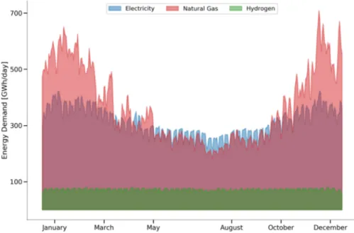
Typical daily aggregated profiles of electricity, natural gas and hy-drogen demand are displayed inFig. 2.
4.2.3. CO2budget
The present model includes the power generation, residential and commercial, as well as road and electrified rail transport sectors in their
entirety, while only the industrial subsectors consuming natural gas and hydrogen are taken into account. According to[56], in 1990, the first three sectors were responsible for the emission of 23.6, 20.0 and 25.0 Mt CO2eq, respectively, while emissions associated with the nat-ural gas-based share of industry is estimated to be around 9.0 Mt CO2eq, also accounting for some hydrogen production. The latter figure is obtained based on a 45 TWh demand of natural gas in the industrial sector [52] and an associated 0.2 tCO2eq/MWhth specific emission value[57]. Thus, the 1990 CO2reference emissions level for the system studied with the proposed model amounts to 77.6 Mt CO2eq, or 51.8% of total national emissions at the time. The carbon dioxide budget considered in all scenarios is set to achieve a reduction of 80% from 1990 levels, or 15.5 Mt/yr.
4.2.4. Imports & exports of energy & commodity
In this case study, both electricity imports and exports are con-sidered, whereas only imports of natural gas and hydrogen and exports of carbon dioxide, respectively, are envisaged.
The electricity import/export capacity is set to 6.5 GW, which is consistent with planned interconnection developments in the 2020s [48]. In addition, the annual electricity imports allowed in the model correspond to roughly 11.5 TWh, amounting to approximately 10% of the total, cross-sector annual electrical load. The costs of electricity imports/exports are based on wholesale prices from the ELIX index of EPEX[9]. This assumption is further discussed later on.
The natural gas import capacity is set to 90 GW, which roughly corresponds to the input capacity of the Belgian natural gas network. The annual imports budget is virtually unconstrained. The natural gas import price time series is derived from medium-term forecasts for the Belgian gas hub, computed and provided by the Belgian natural gas TSO. The Belgian gas hub is particularly well-connected and can resort to a variety of supply options, resulting in an average natural gas price around 12€/MWh in the case at hand.
The import of hydrogen is assumed to be in the form of multi-weekly hydrogen deliveries by tankers. Tankers are assumed to have a capacity of 105m3 and transport hydrogen compressed at 700 bars, such that each tanker delivers 165 GWh over the course of 24 hours. It is further assumed that at most three fixed delivery slots are available each week, which is consistent with the 110 slots made available at the liquefied natural gas (LNG) terminal at Zeebrugge in 2018. As a result, maximum annual hydrogen imports total 25.74 TWh. The hydrogen
import cost is estimated to be around 160€/MWh [9]. It is worth mentioning that no hydrogen terminal currently exists in Belgium but estimating the associated costs is beyond the scope of this study, as the primary goal is to assess the extent to which hydrogen imports are fa-voured over local production.
Finally, it is assumed that carbon dioxide can be exported to a se-questration site at a maximum rate of 3.5 kt/h, such that roughly 30 Mt can be exported annually. Volumetric flows corresponding to this ex-port rate are equal to 9 × 10³m3/h for supercritical carbon dioxide or 1.13 × 10⁵m3/h for gaseous carbon dioxide at 15 MPa and 283.15 K [58], which is the pressure at which carbon dioxide exits the direct air capture process [42]. The cost of exporting and sequestrating 1 t of carbon dioxide is estimated to be around 2€[43]. The export rate as-sumption will be found to have a non-negligible impact on results and will therefore be further discussed later.
4.2.5. Key economic and technical parameters
The main technical and economic parameters of the technologies available in the proposed model are shown inTable 1. A complete list of all parameter values along with references is provided in[9]. At this stage, making a few comments about values displayed inTable 1is in order.
For power generation technologies, the electrical efficiency is pro-vided. For conversion technologies, the overall process efficiency is listed. For storage technologies, the round-trip efficiency is given, while batteries also have a non-negligible self-discharge rate, shown in par-entheses. For carbon capture technologies, the value represents the maximum share of CO_2that may be captured.
All CAPEX are expressed per unit of power capacity (GW) for all dispatchable and conversion technologies, energy capacity (GWh) for storage technologies except carbon dioxide, or flow rate (kT/h) for carbon capture and storage technologies, respectively. Fixed O&M costs are reported on a yearly basis using the same units. Variable O&M costs exclude fuel expenses and are reported per unit energy (GWh). The carbon dioxide storage system is assumed to be a man-made, industrial-sized CO2buffer of 100 kt. Its CAPEX is expressed per kt of CO2stored. The cost of post-combustion carbon capture technologies depends on the fuel that is used by the underlying technology. In this regard, a distinction is made between technologies running on natural gas, e.g. OCGT, CCGT, CHP, SMR, and others, e.g. biomass and waste power plants, for which a coal-based post-combustion carbon capture set-up
Table 1
Key technical and economic parameters of technologies considered. Units are discussed in Section4.2.5.
κ0(κmax) η CAPEX FOM (VOM) Lifetime
GW/GWh/kT h−1 % M€ M€ years
Solar PV 4.0 (40.0) 510 22.3 (N/A) 30
Onshore wind 2.8 (8.4) 910 37.8 (N/A) 30
Offshore wind 2.3 (8.0) 2,000 8.8 (N/A) 30
Gas-fired plants (CCGT) 0.0 (13.5) 58.0 830 27.8 (0.0042) 25
Gas-fired plants (OCGT) 0.0 (13.5) 41.0 560 18.6 (0.0042) 25
CHP 1.8 (N/A) 49.0 40.0 (0.0)
Waste PP 0.3 (N/A) 22.7 175.6 (0.0248)
Biomass PP 0.9 (N/A) 28.1 102.9 (0.0051)
Hydrogen fuel cell 0.0 (13.5) 50.0 2,000 100.0 (0.0) 10
Electrolyser 0.0 (13.5) 62.0 600 30.0 (0.0) 15
Methanation plants 0.0 (13.5) 78.0 400 20.0 (0.0) 20
Steam methane reformers 0.0 (13.5) 80.0 400 20.0 (0.0) 20
Post-combustion CC (NG) 0.0 (4,000.0) 90.0 3,150 20
Post-combustion CC (other) 0.0 (2,000.0) 90.0 2,160 20
Direct air CC 0.0 (1,000.0) 7,500 25.0 (0.0) 30
Battery storage (p) 0.0 (2,500.0) 108 5.4 (0.0) 20
Battery storage (e) 0.0 (5,000.0) 85.0 (99.9) 326 16.3 (0.0) 10
Pumped-hydro storage (p) 1.3 (N/A)
Pumped-hydro storage (e) 5.3 (N/A) 81.0 45.0 (0.008)
Hydrogen storage (e) 0.0 (10,000.0) 96.4 11 0.55 (0.0) 30
Natural gas storage (e) 8,000.0 (N/A) 99.0 0.0025 (0.0)
was used as a proxy in the estimation of associated costs.
Though not shown inTable 1, the costs of energy not served (also known as value of lost load) for electricity, hydrogen and natural gas are set to 3000€/MWh, 500€/MWh and 500€/MWh, respectively. The value used for electricity is consistent with values reported for private end users[59](Fig. 3, left panel in the aforementioned reference), al-though lower than those listed for economic (industrial) consumers. From a modelling standpoint, however, the values must also be selected to promote adequacy, i.e. the costs incurred when failing to serve the energy demand should exceed the investment and operating costs re-quired to deploy, operate and maintain technologies allowing to supply the energy demands. In particular, the value of lost load is set higher for electricity than for other carriers as the electricity system must be ba-lanced at all times, whereas local imbalances can be tolerated in the gas system. Bearing this in mind, the values for natural gas and hydrogen were selected after consulting the Belgian natural gas TSO. Finally, a carbon price of 80€/t has been applied in each scenario.
4.3. Results
Fig. 3displays the installed capacities of all technologies which are sized in each scenario. Hence, CHP, biomass, waste and pumped-hydro power plants, whose capacities are fixed and shown inTable 1, do not appear in Figure 3. Then,Tables 2–4gather the capacities of carbon capture and storage technologies, system and energy costs, broken down by carrier, as well as volumes of energy imports and energy de-mand not served, respectively. InTable 3, the system-wide cost includes all investment and operating costs, as well as all expenses stemming from energy and commodity imports/exports, and energy demand not served. The costs of carriers are reported solely with respect to the corresponding volumes of demand served. Thus, for any given carrier, its cost is obtained by dividing the expenses resulting from all tech-nologies producing it and importing it by the demand for this carrier that was served. Moreover, when deployed, PCCC costs are included in electricity and hydrogen costs. Carbon dioxide costs are obtained by computing PCCC and DAC costs and dividing by the amount of CO2 captured. Finally, it is worth mentioning that DAC costs are reported without energy-related expenses. Now, general observations are made before results are analysed and discussed for each scenario.
Firstly, the renewable potential is fully exploited in each of the first four scenarios, which explains the fact that the installed capacity of
renewable-based power generation technologies only changes in sce-nario 5. Furthermore, the total installed capacity of dispatchable power generation, shown inFig. 3, remains remarkably constant across all
Fig. 3. Deployed generation, conversion and storage capacities across the five considered scenarios. For each scenario, the first, second, third and fourth bars
represent renewable-based power generation, dispatchable power generation, other conversion and storage technologies, respectively, besides CO2storage.
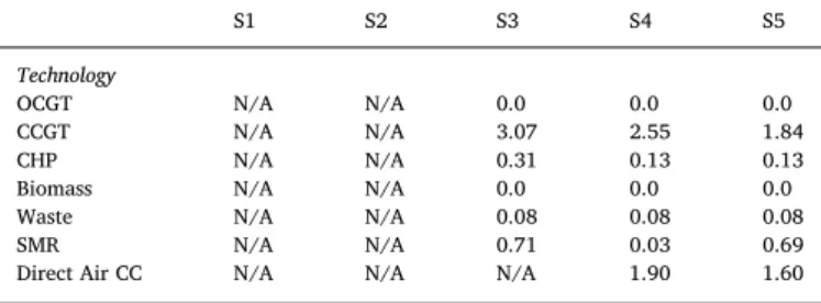
Table 2
Post-combustion and direct air carbon capture deployments for each of the five scenarios. Figures representing capture rates are expressed in kt/h.
S1 S2 S3 S4 S5
Technology
OCGT N/A N/A 0.0 0.0 0.0
CCGT N/A N/A 3.07 2.55 1.84
CHP N/A N/A 0.31 0.13 0.13
Biomass N/A N/A 0.0 0.0 0.0
Waste N/A N/A 0.08 0.08 0.08
SMR N/A N/A 0.71 0.03 0.69
Direct Air CC N/A N/A N/A 1.90 1.60
Table 3
System-wide and electricity (E), natural gas (NG), hydrogen (H2) and carbon dioxide (CO2) sub-system costs associated with the five considered scenarios. Carbon dioxide costs are reported without energy-related expenses.
Unit S1 S2 S3 S4 S5 System b€/year 67.1 50.8 41.2 14.7 9.6 E €/MWh 67.1 52.4 40.8 46.0 45.6 NG €/MWh 11.6 11.7 11.8 12.0 12.0 H2 €/MWh 164.3 146.8 25.0 163.0 24.9 CO2 €/t N/A N/A 35.1 49.2 46.6 Table 4
Import and energy not served (ENS) volumes of electricity (E), natural gas (NG) and hydrogen (H2) across the five considered scenarios (TWh).
S1 S2 S3 S4 S5 E Imports 57.2 57.2 57.2 57.2 57.2 ENS 0.0 0.0 0.0 0.0 0.0 Curtailment 1.7 3.4 18.6 8.3 94.7 NG Imports 365.8 365.8 855.4 1124.6 1124.5 ENS 545.6 390.8 347.1 0.0 0.0 H2 Imports 128.7 120.8 0.5 127.9 0.1 ENS 2.0 1.9 0.0 0.1 0.0