Simple Adaptive Methodology for Chattering-free
Sliding Mode Control
Hancheol Cho, Gaëtan Kerschen
Department of Aerospace and Mechanical Engineering University of Liège
Liège, Belgium
[email protected], [email protected]
Abstract—This paper presents a new adaptive methodology for sliding mode control of a nonlinear dynamical system in the presence of unknown, but bounded uncertainties. A continuous control law is first developed to compensate for the uncertainties and this Lyapunov-based approach eliminates chattering by replacing a discontinuous signum function with a continuous function. By investigating the relation between the estimated gain with respect to the real unknown uncertainties and the resultant sliding variable, a new adaptive tuning law is obtained to ensure that the gain update is performed in real time and the resulting error is bounded within a user-specified value. The proposed adaptive algorithm is simple and easy to implement, and an inverted pendulum problem serves to demonstrate the accuracy and effectiveness of the control methodology proposed herein.
Keywords—adaptive sliding mode control; chattering; nonlinear uncertain systems; Lyapunov stability
I. INTRODUCTION
The control methodology applied to a real-life situation must be robust in that it should still satisfy desired control requirements in the presence of uncertain parameters and disturbances. Sliding mode control (SMC) is widely adopted for controlling nonlinear uncertain systems in various fields of study [1-4]. The use of a discontinuous function and high control gain characterizes conventional sliding mode control, which guarantees good robustness and the finite-time convergence. However, it inevitably leads to the well-known “chattering” phenomenon, which may damage actuators, degrade the control performance, and sometimes make the system unstable.
The most common way to reduce chattering is the use of a boundary layer [5,6]. However, as noted by in [7] this approach sometimes does not completely remove chattering so a proportional, integral, derivative (PID) control of sliding surface function is proposed [7]. Some problems can be handled using this approach, but the existence of the PID control gains satisfying the reachability condition is not always guaranteed. Another method to suppress the chattering phenomenon is to use higher order sliding mode control (HOSMC) [8-9] or the super twisting algorithm [10]. Although HOSMC indeed reduces chattering, its algorithm is generally complicated to realize in real, actual systems. In [11,12] simple continuous SMCs are derived that completely avoid chattering.
Since a continuous function is employed, robustness is compromised (i.e., the sliding variable does not exactly converge to zero) but the errors can be made as arbitrarily small as desired. One drawback of this continuous SMC is that it requires prior knowledge about uncertainties bound. In fact, the other approaches (boundary layer approach, PID-type SMC, HOSMC) also have the same problem. Adaptive sliding mode control [13,14] is proposed to ensure an adaptation of the control gain without the knowledge of the uncertainty bounds. The main focus lies in the adaptation of the gain to the smallest possible value while still sufficiently counteracting the uncertainties. Nonetheless, since a discontinuous function is used in the controller, chattering is still present although it can be mitigated.
The objective of this paper is to propose a simple adaptive law for robust control of a nonlinear uncertain system whose uncertainty bounds are not known. After deriving a continuous SMC, a relation between the estimated gain and the resultant sliding variable is investigated to develop a new adaptive tuning algorithm that still guarantees the bounded error within a user-specified value. Since only a continuous function is used in the controller, chattering completely vanishes. Effectiveness of the proposed controller is verified by simulating a numerical example in which an inverted pendulum is to be controlled within a pre-defined error bound under uncertain system parameters and disturbances.
II. PROBLEM STATEMENT
Let us first consider the nonlinear uncertain system
, ( ) , ( ) , ( ) , t t t t t u t y t h t x f x g x x where
n t Rx is the state vector, u t R
is the control input, y t R
is the system output, and h x
is the output function. Functions f
t,x
and g
t,x
0 are smooth and uncertain, and they are assumed to be bounded for x . Denoting the error vector e t
as e t
y t
yd
t , where yd
t is the desired output, then the sliding variable
s t is defined as follows:
( 1)
( 2)
1 2 1 : n n n , s t e t e t e t e t where the constant coefficients n1, , 2, 1 comprise a Hurwitz polynomial. In (3), the superscript (n 1) denotes the (n 1)th time derivative. Assuming that the sliding variable
s t admits a relative degree equal to 1 with respect to u t
and one can represent ( )n
y t in the form of
( )
, , ,
n
y t t x b t x u t
where
t,x
and b t
,x
0 are unknown, then the system (1) does not have internal dynamics because the relative degree of the system (1) is equal to the system’s order. From here on for brevity, the arguments of the various quantities will be suppressed unless required for clarity. Differentiating (3) with respect to time yields
( ) ( 1) 1 2 1 ( ) ( ) ( 1) ( 1) 1 2 1 ( ) ( 1) ( 1) 1 2 1 , n n n n n n n d n d d d n n n d n d d d s e e e e y y y y y y y y bu y y y y y y y z bu where
( )
( 1) 1 2 1 , : n n d n z t y e e e x is defined.The functions z t x
,
and b t x
,
are supposed to be such that z t
,x
, 0bmbbM. It is noted that the positive constants , b , and m b exist, but M are not known. The aim is then to propose a new sliding mode controller u t
that does not suffer from chattering “without” any information on uncertainties.III. CHATTERING-FREE SLIDING MODE CONTROL
First, the bounds , b , and m b in (6) are assumed to be M
known in this section. An adaptive tuning law will be given in the next section. Let us define a Lyapunov function L as
1 2
. 2
L s
Its time derivative is given by
Lsss z
bu
, where (5) is used. Consider the following control law:
, m u s b
where is a (small) positive constant which will be shortly
explained in detail. Then, the following theorem holds.
Theorem 1 Given the nonlinear uncertain system (1) controlled by (9), the state trajectories of (1) are forced to move from initial conditions to the region s t
in a finite time and remain in the region. ■ Proof. Substituting (9) into (8), one gets 2 2 1/ 2 1 2 1 2 , m m m m b b L sz s s s b b s b b s s s b b V where 2 1 m b s b
is positive in the region s t
holds. Hence, the state trajectories of (1) controlled by (9) converge to the region s t
in a finite time and remain in the region thereafter, which completes the proof. ■ Corollary 1 Let us consider a second-order
n 2
system. If the sliding variable s given by s e 1e is bounded bys , then as time progresses, the actual error e and its time derivative e are eventually bounded by e / 1 and
2
e , respectively. ■ Proof. From the definition of s , one has
e 1e
and let us first consider the following condition:
e1e.
0 1
0
1 1 exp , e e t t where e0:e t
0 is defined. Next, consider the following condition: e 1e,
then, following the same procedure one can obtain a similar result. 0 1
0
1 1 exp . e e t t Combining the two, the error is bounded by
0 1 0 0 1 0 1 1 1 1 exp exp . e t t e e t t
Since is positive, the exponential term decays rapidly and 1
1 1 . e
Next, using the above inequality and the definition of s , it is straightforward to show that
2 e 2 ,
and this completes the proof. ■ IV. NEW ADAPTIVE RULES FOR CHATTERING-FREE SLIDING
MODE CONTROL
In the previous section, it is shown that the use of the control law (9) makes the sliding variable bounded by s . Although it does not guarantee that the sliding variable will be effectively equal to zero, one can always choose a small number to guarantee a pre-defined upper bound.
One drawback of the control law (9) (and the conventional sliding mode controller) is the requirement on the knowledge of the uncertainty bounds. In practice, it is generally very difficult to accurately estimate these bounds. However, one can observe from (9) that increasing the value of or decreasing the value of b is mathematically equivalent to decreasing the m value of , resulting in smaller s , and accordingly, smaller
errors. For example, assume that one could obtain exact values for the bounds and b , then one has sm . Since one does not know the exact values for the bounds in practice, however, suppose that the estimates and 0 bm,0 are tried. If is the
(unknown) number that equates the two terms 0/bm,0 and /bm
by 0/bm,0 /bm, then the sliding variable will be bounded by s / . More generally, let us assume that s is 1 the sliding variable when the first estimates and 1 bm,1 are used and s is the one when the second estimates 2 and 2 bm,2 are employed, while the same is assumed in both cases.
Then, the following equality holds:
1
2
1 2 ,1 ,2 sup sup . m m s s b b One can also deduce from (9) and (19) that the maximum value of the magnitude of the control input (i.e., max u
) is unchanged by the choices for the bounds of and b , which mwill be used to derive an adaptive law. This observation provides us with one method to estimate the quantity /bm. Assume that rough estimates for the bounds and bm are applied and the resultant measured sliding variable s is bounded by so that s . Then, the real (unknown) gain value * * /bm can be calculated by * * , m m b b
where is the desired bound for s . Although (20) can serve
as a new method for the estimation of the bounds, the following adaptive rule provides us with a succinct solution for “real-time” tuning.
Adaptive Rule Let 0 and bm,0 be the initial estimates. The real-time adaptive law for the gain / b for the control law (9) is given by the following rules:
(i) At each instant of time, s t
is compared with . When
s t , /bm maintains its current value (with and 0 bm,0
as the initial conditions). In discrete time implementation, it can be expressed as ( 1) ( ) ( ) , if . k k k m m s b b
where the superscript “k” denotes the quantity at the kth scan time.
(ii) If s t
at time t, then /bm should be updated to be multiplied by s t
/ and added by a small positive constantm
( 1) ( ) ( ) ( ) , if . k k k k m m m s K s b b
Finally, /bm determined by (21) and (22) should maintain its
maximum of all past values. ■ Proof. Roughly speaking, when s t
holds, it means thatthe current gain /bm is not enough to suppress s t
less than . Then, the adaptive law (22) increases the gain /bm until the condition s t
is achieved, which is guaranteed by (20). It is noted that if the initial gain 0/bm,0 is greater than or equal to the real unknown gain */bm*, then (21) holds and the gain /bm remains constant. On the other hand, if the selected 0/bm,0 is smaller than * */bm
, the gain /bm
increases by following (22) until * * /bm /bm
is attained. For brevity, the notation K /bm is used for the current gain value. Likewise, the initial gain is denoted by
0 0/ m,0
K b and the real gain is written as * * * / m
K b . Now, let us define the following Lyapunov candidate function:
1 2 1
*
2 , 2 2 V s K K where is a positive constant. It should be noted that the
condition *
0
K KK is always satisfied because the time derivative of K is always zero or positive by (21) and (22).
The time derivative of the Lyapunov function (23) yields
* * * * 1 1 1 1 , V ss K K K s z bu K K K bK s z s K K K bK s s K K K where z is used.First, the case when s is considered. Then, (24) satisfies
* * * * * 1 1 1 , s V s bK K K K s bK K K K s bK s bK s K K b s K where *
/ 1 0 s b Km b bm is defined and * * KK KK is used because * KK . Now, a parameter K 0 is introduced in (25) as * * * * 1 , s K K s K V s K K b s K K K K K s K K where KK*
b sK/ K
is defined. Finally, (26) leads to
* * 1/ 2 2 2 2 2 min 2, 2 2 2 , s K s K K K s V K K s V where 2 min
s, K
0.It is noted that it is always possible to make 0 by a proper selection of that is not included in a design
parameter of control. The condition 0 yields
1 K 0 . K K b s K b s
Using (22), K can be approximately written as
1 , m s K K K t
where t is the step size. With (29), (28) becomes
1 . m K s K K t b s Now, with the condition s , can be selected so that it is
smaller than the right hand side of (30), or
max , m M K K t b where t is the maximum step size and b is the upper bound M for b as noted in (6).
Finally, from (27), one has V V1/ 2 V1/ 2, and hence, finite time convergence to the region s is guaranteed from the time when s starts to exceed .
Next, let us consider the case when s holds. In this case, the gain K maintains its previous value by (21) and
may not be positive so that V is sign-indefinite and s may exceed . However, as soon as it becomes larger than ,
1/ 2
V V holds and s will be again bounded by s in a finite time, as shown earlier.
In brief, the adaptive rule (21) and (22) guarantees that the sliding variable will be bounded within the region s
in a finite time from any initial condition and will remain in the region thereafter, which completes the proof. ■
The adaptive rule (21) and (22) is alternatively represented in a more compact form like the following:
(i) At each instant of time, /bm is compared with u t
. When /bmu t
, /bm maintains its current value. (with0
and bm,0 as the initial conditions) In discrete time implementation, it can be expressed as
( 1) ( ) ( ) ( ) , if . k k k k m m m u b b b
(ii) If /bmu t
at time t, then /bm should be updated to u t
Km with K being a positive constant. In discrete m time implementation, it can be expressed as ( 1) ( ) ( ) ( ) , if . k k k k m m m u K u b b
It is not difficult to show that (32) and (33) are identical with the adaptive rule (21) and (22) using the definition of the control law (9).
V. NUMERICAL EXAMPLE
The new adaptive SMC proposed in this paper is applied to an inverted pendulum problem with uncertain parameters and disturbances. Numerical integration in this example is carried out in the Matlab/Simulink environment, using a fixed time step of 0.001 second and the ode4 Runge-Kutta integrator.
Let us consider an inverted pendulum system whose equation of motion is described by
x c t x
acos
x bud t
. The (unknown) parameters of the actual system are a 3.2,
0.5 0.2sin
c t t , b 1.1 , and the disturbance is
2sin 0.1
d t t . Suppose that the output y is yx and the desired trajectory is yd sin 0.2
t
. Since (34) is a second-order system, the sliding variable is given by s t
e t
1e t
, where 1 2 is assumed. Also, the control law (9) with
0.01
is used for the simulation so that the resultant error is bounded by e / 10.005 by Corollary 1. The initial conditions are x
0 0 and x
0 0.2, and e
0 0 and
0 0e are assumed.
Case 1. Since one cannot exactly measure the uncertainty and the disturbance, let us first try ˆ 7 and ˆb m 2. Figure 1 shows the time history of the sliding variable s t
, the error
e t , and the required control input u t
. It is observed thats is not bounded by , and sup
s 0.01326 which is greater than . With this observation, the real uncertainty canbe calculated using (20): 4.6423. m m b b
Case 2. Now one can choose 4.6423 and b m 1 obtained in (36). In Fig. 2, s t
, e t
, and u t
are depicted. As desired, s is precisely bounded by and e is bounded by1 /
. Also, the magnitude of the control input u remains
almost the same, when compared with Case 1.
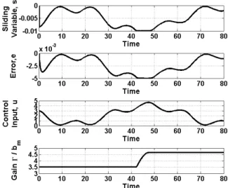
Case 3. In this case, the adaptive law given by (32) and (33) with K m 0.001 is verified. It is noted that K should be m small enough not to produce any sudden rise in the control gain, the sliding variable, or the control input. The result is shown in Fig. 3. As in Case 1, 7 and b m 2 is chosen, hence, /bm3.5 at the initial time. At t 42.1755, u starts to exceed this value. /bm is accordingly updated by following uKm, and has the final value of /bm4.6433 which is also equal to max
u Km. Although it is initially under-estimated, the uncertainty /bm is successfully tuned in real time. As a result, s is bounded by and e is alsoalways maintained less than as desired. In addition, the / 1 adaptive controller does not suffer from chattering.
Fig. 1 s t , e t , and u t when 7 and b m 2
Fig. 2 s t , e t , and u t when 4.6423 and b m 1
Fig. 3 s t , e t , u t , and /bm when the adaptive rule (32) and (33) is
applied
VI. CONCLUSIONS
A new adaptive tuning method for continuous sliding mode control is proposed for an uncertain nonlinear system whose system parameters and disturbances are not known. The developed algorithm successfully guarantees that the error remains within a user-specified bound without knowing uncertainty bounds. The methodology exploits the fact that the maximum of the magnitude of the control input is independent of the choice of the estimates for the uncertainty bounds. The information on the magnitude of the control input is employed for on-line tuning so that the gain update is readily implemented in real time, which eases the application of the suggested algorithm to real-world systems. The inverted pendulum system validates the efficacy of the new adaptive sliding mode controller.
REFERENCES
[1] M. G. R. Neila and D. Tarak, “Adaptive terminal sliding mode control for rigid robotic manipulators,” Int. J. Auto. Comp, vol. 8, pp. 215–220, 2011.
[2] M. Ertugrul, O. Kaynak, and F. Kerestecioglu, “Gain adaptation in sliding mode control of robotic manipulators,” Int. J. Syst. Sci., vo. 31, pp. 1099–1106, 2000.
[3] Y. Heidari and R. N. Rad, “Adaptive robust PID controller design based on a sliding mode for uncertain chaotic systems,” J. Math. Comp. Sci., vol. 4, pp. 71–80, 2012.
[4] T. Massey and Y. Shtessel, “Continuous traditional and high-order sliding modes for satellite formation control,” J. Guid. Control. Dyn., vol. 28, pp. 826–831, 2005.
[5] J. J. Slotine and S. S. Sastry, “Tracking control of nonlinear systems using sliding surfaces with application to robot manipulator,” Int. J. Control, vol. 38, pp. 465–492, 1983.
[6] J. A. Burton and A. S. Zinober, “Continuous approximation of variable structure control,” Int. J. Syst. Sci., vol. 17, pp. 875–885, 1986. [7] M. Li, F. Wang, and F. Gao, “PID-based sliding mode controller for
nonlinear processes,” Ind. Eng. Chem., vol. 40, pp. 2660–2667, 2001. [8] S. Laghrouche, F. Plestan, and A. Glumineau, “Higher order sliding
mode control based on integral sliding surface,” Automatica, vol. 43, pp. 531–537, 2007.
[9] A. Estrada and L. M. Fridman, “Integral HOSM semiglobal controller for finite-time exact compensation of unmatched perturbations,” IEEE Trans. Automat. Contr., vol. 55, pp. 2645–2649, 2010.
[10] A. Levant, “Sliding order and sliding accuracy in sliding mode control,” Int. J. Control, vol. 58, pp. 1247–1263, 1993.
[11] F. E. Udwadia, T. Wanichanon, and H. Cho, “Methodology for satellite formation-keeping in the presence of system uncertainties,” J. Guid. Control. Dyn., vol. 37, pp. 1611–1624, 2014.
[12] H. Cho, T. Wanichanon, and F. E. Udwadia, “New continuous control methodology for nonlinear dynamical systems with uncertain parameters,” Proceedings of the 1st ECCOMAS Thematic Conference on International Conference on Uncertainty Quantification in Computational Sciences and Engineering, Crete, Greece, May 2015. [13] F. Plestan, Y. Shtessel, V. Brégeault, and A. Poznyak, “New
methodologies for adaptive sliding mode control,” Int. J. Control, vol. 83, pp. 1907–1919, 2010.
[14] V. I. Utkin and A. S. Poznyak, “Adaptive sliding mode control,” Advances in Sliding Mode Control, Springer Berlin Heidelberg, 2013, pp. 21–53.
[15] T. H. Grönwall, “Note on the derivatives with respect to a parameter of the solutions of a system of differential equations,” Ann. of Math., vol. 20, pp. 292–296, 1919.