Size-adaptive spherical receptor acceleration method for acoustical ray tracing

Size-adaptive spherical receptor acceleration method for

acoustical ray tracing

S. Lesoinne and J.-J. Embrechts

University of Li`ege - INTELSIG, Institut Mont´efiore, Sart-Tilman, Batiment 28, 4000 Li`ege,

Belgium

Randomized ray tracing in room acoustics can be used to compute echograms, but the results computed at the receptor are affected by statistical errors.

To decrease these statistical errors, the usual solution is to increase the number of rays, but this also increases the computation time. Another solution is to increase the receptor size, but this lowers the spatial resolution of the computed sound field, which is particularly important for the early part of the echogram.

In order to decrease the computation time and keep a sufficient resolution, the method proposed in this paper is based on a progressive modification of the receptor size (spherical type) as long as the ray’s travel grows. At the same time, the number of rays into the room can be decreased as the sound ray lengths increase while keeping the statistical errors more or less constant. The consequence is that the sound field spatial resolution evolves from “precise” at the beginning of the echogram to “rough” at its end.

The first applications of this new method show a significant gain of CPU time.

1

Introduction

Ray tracing is one of the most popular methods to compute sound fields and room impulse responses. There are numerous ways to implement ray tracing algorithms [1,2], most of them trying to get the most accurate results within the shortest computing time.

Among all these methods, randomized ray tracing consists in simulating the travel of a great number of sound rays in the volume of the room, these rays being originally emitted by the source in random directions. To compute the sound pressure levels (SPL) at a given location in the room, a receiving surface or a spherical receiver are defined at that particular location, with the function of collecting the sound rays’ energy passing nearby and recording their time of arrival. Reference [3] recalls how this can be done in a formal way for a receiving surface. In this paper, spherical receiver will be used.

This last reference also gives a description of the unavoidable statistical errors on the computed results. Their magnitude is mainly influenced by two parameters: the number of emitted rays and the area (or volume) of the receiver. Increasing the number of rays decreases the statistical errors, but also leads to a greater computing time. Also, increasing the size of the receiver results in a better statistical precision, but decreases the spatial resolution of the computed SPLs.

A compromise must therefore be found between accuracy, computing time and spatial resolution. The method proposed in this paper is based on the consideration that spatial resolution is mainly required for the calculation of sound pressure distributions in the room and the early part of the echograms. Both results are mainly dependent on the initial part of the sound rays’ paths into the room. To ensure the accuracy of the mid- and late part of the echograms, while keeping the number of rays unchanged, it is therefore suggested to continuously modify the size of the receiver, as long as the ray’s travel grows.

2

SPL at the spherical receiver

The following expression of the squared rms pressure at a spherical receiver will be derived assuming specular reflections at all surfaces. This expression can be extended for diffusely reflecting surfaces, applying the same method as in ref. [3], but this will not be shown here to avoid too long mathematical developments.

If we call R’, a receiving point within the sphere, the squared rms pressure at R’ can be expressed by:

e

p

Ns mri i i i eff

r

S

W

c

R

− =

∑

=

0 2 0 2

4

(

)

)'

(

ρ

_π

(1)

In this equation, Ns is the total number of image sources (theoretically infinite) which are active at R’, i=0 being the real source; ri is the distance between R’ and the image source number i, and m is the air absorption coefficient (nepers/m) at the frequency at which the calculation is done.

W(Si)/4π is the intensity (watts/steradian) of the image source in the direction of the receiver R’. It can be more generally replaced by:

W S

I

a

I

i i i i i i i i i i

( )

( , ) (

) (

)

( , ) ( , )

4

_π

θ φ

1

α

1

1

α

2

θ φ

θ φ

=

−

−

=

K

(2) i.e. the product of the intensity emitted by the real source in the direction of the sound ray defined by the spherical coordinates (θi,φ i) and representing the travel from Si to R’, and the reflection coefficients (1-αki) of all the surfaces hit by this sound ray (see figure 1).

Fig.1 Propagation path of the sound ray, emitted from the real source S, and representing the travel from the image

source number i to the receiver point R’.

R is the center of the spherical receiver V, while rin and rout are the lengths of the total path between S and, respectively,

the entrance in and output from the sphere.

The averaged squared rms pressure for all the receiving points lying inside the spherical receiver V is obtained by integrating equation (1) for all the angles (θi,φi) leading to this sphere and the variable ri being comprised between rin

and rout (see figure 1). Considering that the elementary volume

dV

=

r

i2

sin

θ

i

d

θ

i

d

φ

i , the integral over ri only

concerns the exponential factor.

Furthermore, all the image sources share the same spherical coordinate system (θ,φ) centered on the real source (see figure 1) and, for each of them, the limits of integration can be extended to the whole solid angle, provided that we introduce the function δk(θ,φ) which is equal to 1 if the sound ray emitted in the direction (θ,φ) crosses the spherical receiver between the kth _{and (k+1)}th _reflections (otherwise δk=0). Finally, the following expression is obtained for the averaged square rms pressure:

∫

∫

=

ρ

π

φ

π

ν

θ

φ

θ

θ

0 2 0 0 2

sin

)

,

(

)

(

R

_V

c

d

d

p

_eff (3) with:

⎟

⎠

⎞

⎜

⎝

⎛

_⎟

⎠

⎞

⎜

⎝

⎛

₋

=

∑

∞ = − − 0

1

)

,

(

)

,

(

)

,

(

)

,

(

k r m r m k k

e

e

out in

m

a

I

θ

φ

θ

φ

δ

θ

φ

φ

θ

ν

(4)

Note that rin and rout are functions of (θ,φ).

As explained in [3], this exact expression is approximated in the randomized sound rays algorithm by:

∑

=

=

N j j j

NV

c

V

p

1 0 2

)

,

(

4

)

(

π

ρ

ν

θ

φ

(5)

with N being the total number of rays emitted by the source, and (θj,φj) the initial (random) direction of the sound ray number j.

Eq. (3) to (5) form, in fact, the basis of the randomized sound ray method. They have been established under the assumption that the spherical receiver is small enough to not interfere with the surfaces of the room. For most applications in room acoustics, spheres with diameter of about 1 meter are used, so that this assumption can be satisfied. However, if we want to enlarge the size of the receiver as suggested in the introduction, we first have to update these formulas. Fortunately, it is shown in the following that (3) and (5) are still valid, even if there are reflecting surfaces inside the sphere.

Fig.2 Propagation path of the sound ray, emitted from the real source S, and representing the travel from the image

source number i (order k) to the receiver point R’. V represents the image of the room corresponding to this image source, rin and rout have the same signification as in

fig.1, while r1 and r2 delimit the portion of the sound ray inside the room, between reflections of order k and (k+1). To show this, we can consider a volume receiver of any size, spherical or not, intersecting one or several surfaces of the room. In the following, we take as an example the situation where the volume of the receiver is extended to the whole volume of the room (figure 2).

In figure 2, the image of the room corresponding to the source image number i has been drawn. If we use the same spherical coordinate system (θ,φ,ri) as before, we must now consider that the function δk not only depends on (θ,φ), but also on ri. Indeed, the path between rin and r1 has no real signification, since the corresponding sound ray only exists between r1 and r2. So is the path between r2 and rout.

Therefore, Eq. (3) and (4) remain valid, on the condition that rin and rout are now replaced by the length of the sound ray to the reflection number k and to the reflection number (k+1), respectively.

Compared to the small spherical receiver, averaging over the whole volume of the room does not necessitate extra work to compute the intersections of the sound ray with the volume, since r1 and r2 are already computed by the sound ray algorithm.

To compute echograms, Eq. (3) to (5) are restricted to predefined time intervals of duration Δt. For the small spherical receiver, the length of the sound ray between rin and rout determines the time interval in which the contribution takes place. However, for large volume receivers, an additional difficulty is that the distance between r1 and r2 may cover several time intervals (distances covering 100ms of propagation are not unusual in large rooms). Therefore, a procedure must distribute the sound ray’s energy between those time intervals.

3

Variable size spherical receptors

Increase of the spherical receiver size is done from a chosen value to another one depending on the ray length. It implies some modifications of the ray tracing algorithm such as:

- Temporal spreading of each ray contribution. The time spent by a ray in the receiver may become bigger than a temporal interval Δt of the

echogram. Therefore, this ray participates to more than one Δt at once and the ray contribution to a receiver must be spread on all concerned Δt. - The modification of the entry and exit points of the

receiver: when the receiver intersects at least one surface, entry and exit points of the receiver may be out of the surface of the sphere.

- Computing the number of rays to keep as the receiver size is changed.

- Stopping of the superfluous rays as the receiver size grows and updating the power of the remaining rays.

Moreover, there exists a homogeneity condition on the acoustical pressure1 _{inside the receiver exists that binds the}

1 _{Needed for estimation of p}

eff² at the sphere center by the mean of the rays contributions over the receiver volume.

ray travel length to the size of the receiver. Also, the volume computation of a truncated receiver requires a modified algorithm. It should be noted that problems of homogeneity of the acoustical pressure inside the receiver can arise due to the existence of more than one acoustical space in the room simulated.

3.1 Spreading of the rays contribution

At first, the entry and exit time intervals (itin and itout) of the ray in the receiver are determined. Then, the ray’s energetic contribution to the receiver is spread according to the ray crossing time of each temporal interval included in [itin, itout]. The ray contribution to the “it” interval is:

ratio receiver

it

E

Time

E

=

(6)

where Eit is the energy received by the time interval “it”, Ereceiver is the total energy received by the receiver and Timeratio is the ratio of the time spent in the time interval “it” versus the time spent in the receiver.

3.2 Entry and exit points

As previously mentioned, if the spherical receiver includes one or more surfaces, the entry and exit points must be updated. If the ray intersects a surface in the sphere, the exit point is their point of intersection. This point is also the “entry point” for the next ray segment. Considering these changes, Eq. (3) remains valid.

3.3 Number of rays to keep

The number of rays has to be decreased, while keeping a constant ray - receiver intersection probability. The number of rays intercepted by a spherical receiver is proportional to Nρ² where ρ is the radius of the sphere. Thus, when this radius changes from ρ1 to ρ2, the number of rays must be divided by (ρ2/ρ1)² to keep the probability unchanged. Since receivers may be truncated, this expression need to be modified using ρ1,equiv and ρ2,equiv where ρi,equiv is the radius of a sphere with a surface equal to the surface of the truncated sphere of radius ρi.

3.4 Computation of the surface and

volume of the truncated receivers

Before starting the sound ray process, the surface of the receiver can be pre-computed by randomly shooting N rays (without reflections) from the receiver center using the following formula:

∑

≈

N i i i

r

N

S

4

π

2

(

_θ

,

_ϕ

)

₍₇₎ where r(θi,φi) is the distance from the receiver center to the element (room surface or receptor edge) having an intersection with ray that fulfils the three following conditions:

- The furthest intersection from the receiver center2 - At a distance to the center d ≤ ρ

- In the accessible part of the room3

2 _{The receiver can include small parts of the room, but it} must reject areas outside the room.

As soon as S is known, so is ρi,equiv.

The volume of the receiver is computed using an equivalent method.

3.5 Stopping the superfluous rays

Only the first N2 rays are kept, according to §3.3 (as the ray shooting is randomized so is the stopping process). Continuing the simulation with N2 rays is equivalent to a new simulation in which the N2 rays would follow the same paths. The power of the N2 rays must be multiplied by N1/N2 to keep constant the global power of the rays at any given time.

3.6 Receiver’s homogeneity condition

To estimate peff² at the sphere center by averaging the rays contributions in the receiver volume, the acoustical pressure homogeneity condition must be respected. In the simple case of a spherical propagation in free field, the receiver pressure disparity can be expressed by:

ρ

ρ

ρ

αρ

_≠

−

+

=

−

=

R

e

R

R

R

P

R

P

R

P

R

P

D

eff eff eff eff dB

),

(

log

20

)

)

(

)

(

(

log

10

)

)

(

)

(

(

log

10

10 2 2 2 10 2 1 2 10 (8)

where α is the air attenuation, ρ the receiver radius, R the distance from the image source to the sphere center, R1 and R2 are respectively the entry and exit points in the spherical receiver of a ray passing by his center.

If the disparity must be limited to a chosen value DdB,choice, the condition to respect [4] when the sphere size is chosen is that:

)

(

choice choice

e

A

e

A

R

choice choice choice αρ αρ

ρ

−

+

≥

(9)

valid in free field and where

) 20 ) 10 ln( ( DdB,choice choice

e

A

=

(10)

If the receiver doesn’t include any obstacle, this condition remains valid out of free field conditions because the reflections on the walls lead to a faster weakening of peff² (this is equivalent to a bigger distance covered in free-field). Since (δDdB/δR) < 0, the disparity inside the receiver is lower than expected in free field.

3.7 Changing receiver radius

Knowing Eq.(9), the ray must have travelled a minimum distance called “threshold distance” before changing the radius of a receiver. All receivers in the room have the same set of radius – threshold couples.

So the size of a receiver is not modified continuously, but step by step starting from its initial size, “threshold 3 _{Non-accessible areas are those where acoustical pressure} is supposed to be zero Pascal. These areas are characterized manually.

distance” after “threshold distance”. This is equivalent to split the ray tracing up in L+1 independent ray tracings relative to the L+1 temporal intervals groups separated by L threshold, where a ray intersects fixed size receiver. One condition for that: the “threshold time”4 _{must be the same} for all frequency bands and it must be a multiple of Δt, the temporal interval.

This split up in L+1 independent ray tracings enable to estimate the statistical error in the classical way for each ray tracing process.

4

Results

4.1 The test room

Simulation has been carried out for example in a long disproportionate room, used by Hodgson [5]. The rectangular room is 110m long, 55m large and 5.5m height. The omnidirectional source is situated at x = 27.5m, y = 10m and z = 1.5m. In this example, a spherical receiver is placed at x = 27.5m, y = 20m and z = 1.75m. The absorption coefficient is the same for all walls α = 0.20. On the contrary, the diffusion coefficient increases as a function of frequency.

4.2 Echograms

In this example, 50M rays were shot and the configuration of the receivers for the test is:

- A simulation of reference with a fixed size spherical receptor of radius 0.25m and with time spreading. This simulation took about 3h40 to complete.

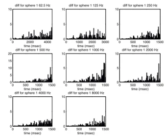
- Three simulations of test with a variable size spherical receptor, each with two couples of radius and threshold as follow [0.25 – 0 ; 1.0 – 300], [0.25 – 0 ; 1.5 – 500], [0.25 – 0 ; 3.0 – 100] with time spreading. These simulations respectively took 2h07 and 3h09 and 48 minutes to complete. Fig. 3 introduces the differences between the value of the echograms obtained with fixed size spherical receiver and those obtained by the growing spherical receiver method. Due to a different power repartition amongst rays, they don’t take the same paths in both simulations which could explain the differences between echograms before the tthreshold. After this time, the differences should be due to the different paths followed by the rays and the bigger receiver size.

As expected, in the few simulations conducted, the acoustical criteria’s (RT, EDT) are kept in a close range between both methods, the maximum deviation being of a few percents.

The more the receiver grows, the less the computation time is. Also, the closer to the origin the tthreshold is, the less the computation time is. To improve the gain of time, multiple couple of radius and threshold can be combined.

4 _{Time spent by a ray to travel the threshold distance.}

0 2000 4000 0

5 10

time (msec) diff for sphere 1 62.5 Hz

0 1000 2000 3000 0

5 10

time (msec) diff for sphere 1 125 Hz

0 500 1000 1500 0

5 10

time (msec) diff for sphere 1 250 Hz

0 500 1000 1500 0 5 10 15 20 time (msec) diff for sphere 1 500 Hz

0 500 1000 1500 0

5 10

time (msec) diff for sphere 1 1000 Hz

0 500 1000 1500 0

5 10

time (msec) diff for sphere 1 2000 Hz

0 500 1000 1500 0

5 10

time (msec) diff for sphere 1 4000 Hz

0 500 1000 1500 0

5 10

time (msec) diff for sphere 1 8000 Hz

Fig.3 Differences in dB of the echograms obtained with fixed size spherical receiver ray tracing (and temporal spreading) and obtained with the growing spherical receiver

method [0.25 – 0 ; 1.0 – 300]. The temporal intervals are bigger at low frequency bands.

5

Conclusion

Using different sizes for a receiver significantly decrease the computation time needed for a simulation, provided that the [radius - threshold] couples are carefully chosen, while keeping the acoustical criteria’s estimation in a close range to their fixed size receiver counterpart.

References

[1] M. Vorländer, "Simulation of the transient and steady state sound propagation in rooms using a new combined sound particle-image source algorithm", J.

Acoust. Soc. Am. 86, 172-178 (1989)

[2] I. A. Drumm, Y. W. Lam, "The adaptive beam tracing algorithm", J. Acoust. Soc. Am. 107, 1405 (2000) [3] J.J. Embrechts, "Broad spectrum diffusion model for

room acoustics ray-tracing algorithms", J. Acoust. Soc.

Am. 107, 2068-2081 (2000)

[4] S. Lesoinne, "Techniques d’accélération du tir de rayons pour la simulation acoustique", DEA Thesis, (2006)

[5] M.R. Hodgson, "Evidence of diffuse reflection in rooms", J. Acoust. Soc. Am., Vol. 89(2), 765-771, (1991)