Cloud filling of ocean colour and sea surface temperature remote sensing products over the Southern North Sea by the Data Interpolating Empirical Orthogonal Functions methodology.

Cloud filling of ocean colour and sea surface temperature remote sensing

products over the Southern North Sea by the Data Interpolating Empirical

Orthogonal Functions methodology

Damien Sirjacobs a , Aida Alvera-Azcárate a , Alexander Barth a , Geneviève Lacroix b , Youngje Park b , Bouchra Nechad b_{, Kevin Ruddick} b_{, Jean-Marie Beckers} a

a

GeoHydrodynamics and Environmental Research, MARE Center, University of Liège, Allée de la Physique 7, B5, 4000 Sart-Tilman, Belgium

b

Management Unit of the North Sea Mathematical Models (MUMM), Royal Belgian Institute of Natural Sciences (RBINS), Gulledelle 100, 1200 Brussels, Belgium

ABSTRACT

Optical remote sensing data is now being used systematically for marine ecosystem applications, such as the forcing of biological models and the operational detection of harmful algae blooms. However, applications are hampered by the incompleteness of imagery and by some quality problems. The Data Interpolating Empirical Orthogonal Functions methodology (DINEOF) allows calculation of missing data in geophysical datasets without requiring a priori knowledge about statistics of the full dataset and has previously been applied to SST reconstructions. This study demonstrates the reconstruction of complete space-time information for 4 years of surface chlorophyll a (CHL), total suspended matter (TSM) and sea surface temperature (SST) over the Southern North Sea (SNS) and English Channel (EC). Optimal reconstructions were obtained when synthesising the original signal into 8 modes for MERIS CHL and into 18 modes for MERIS TSM. Despite the very high proportion of missing data (70%), the variability of original signals explained by the EOF synthesis reached 93.5% for CHL and 97.2% for TSM. For the MODIS TSM dataset, 97.5% of the original variability of the signal was synthesised into 14 modes. The MODIS SST dataset could be synthesised into 13 modes explaining 98% of the input signal variability. Validation of the method is achieved for 3 dates below 2 artificial clouds, by comparing reconstructed data with excluded input information. Complete weekly and monthly averaged climatologies, suitable for use with ecosystem models, were derived from regular daily reconstructions. Error maps associated with every reconstruction were produced according to Beckers et al. (2006). Embedded in this error calculation scheme, a methodology was implemented to produce maps of outliers, allowing identification of unusual or suspicious data points compared to the global dynamics of the dataset. Various algorithm artefacts were associated with high values in the outlier maps (undetected cloud edges, haze areas, contrails, and cloud shadows). With the production of outlier maps, the data reconstruction technique becomes also a very efficient tool for quality control of optical remote sensing data and for change detection within large databases.

Keywords : Remote Sensing ; Cloud Filling ; Quality Control ; Empirical Orthogonal Functions ; Ocean

Colour ; SST ; North Sea ; English Channel

1. Introduction

1.1. importance of cloud filling in remote sensing studies

The objective of this study is to demonstrate the efficiency of a method for reconstruction of complete space-time information for surface chlorophyll a (CHL) and Total Suspended Matter (TSM) from an archive of satellite imagery. The resulting data is better suited for applications such as algae bloom detection or for providing light forcing for ecosystem modelling. In the longer term, comparison of satellite data with

reconstructed fields will contribute to the quality control of satellite data by highlighting suspect or extreme data. The temporal coverage of ocean colour data doesn't allow resolution of high frequency dynamics typical of coastal waters. Wide swath polar-orbiting ocean colour remote sensors acquire data with near-global coverage of the world's oceans and seas every day or, few days. For example, Belgian waters at 51 °N are imaged by

(at around 10h30 local solar time). However, this maximal temporal coverage is greatly reduced by clouds and by sunglint. The usable data is further reduced for environmental conditions for which derived products are considered to be of unacceptable quality because of various processing problems. In particular many problems are associated with atmospheric correction: adjacency effects, high aerosol optical thickness, absorbing aerosols, cloud edge and cloud shadow, sub pixel scale clouds, low sun or viewing zenith angle, etc. As an example, a pixel a few kilometres from the Scheldt river mouth (51.47°N; 3.23°E) was within the swath of the MODIS-Aqua instrument on average 390 times per year for the period 2003-2006, but usable data was retrieved for only 20% of these occasions, that is about 80 times per year. This temporal coverage, although far superior to shipborne sampling methods, is insufficient for many applications.

Total suspended matter products are used by ecosystem modellers to control the light forcing in simulations designed to hindcast or forecast eutrophication as a function of anthropogenic nutrient inputs (Allen et al, 2001; Cugier et al, 2005; Lacroix et al, 2007b). These models require complete spatio-temporal data fields as input. It is important that such inputs contain as much of the high frequency variability as possible since TSM dynamics, such as the clearing of the water column by settling after a storm event, may be responsible for triggering algae blooms (Iriarte and Purdie, 2004; Los et al, 2008). More generally, users of satellite data products, such as marine scientists investigating conditions at specified sampling locations, prefer to receive a continuous time series of data rather than the gappy series typically provided directly from optical remote sensors. There is, therefore, a strong user demand for complete time series and cloud-free maps of CHL and TSM products. This is the primary motivation for the present study which has the objective of generating spatio-temporally complete 3D (horizontal space and time) fields of surface CHL and TSM from a collection of individual instantaneous images of these fields as retrieved from MERIS and MODIS. MODIS Sea Surface Temperature (SST) data are also processed to provide a complementary description of the dynamics of the study area.

As a secondary motivation, it is clear that CHL products derived from optical remote sensing data alone may contain unacceptable errors (Ruddick et al., 2008; Mélin et al., 2007), particularly in coastal waters where non-algal absorbing and scattering components are significant and where atmospheric correction problems are more acute. Multiple solutions to the inverse problem may even be possible (Defoin Platel and Chami, 2007). There is now considerable research activity aimed at determining the quality of derived products. While many studies (Mélin et al., 2007; Doerffer and Schiller, 2000) aim to do this using only the pixel-by-pixel optical remote sensing data, there is a growing interest in using extra information to constrain possible solutions. For example, climatologies of aerosol properties generated from sunphotometer data could be used to constrain the

atmospheric correction to a range of realistic aerosol models encountered in a certain region (desert dusts are not often found at very high latitudes). High TSM concentrations are not likely to occur in deep waters far from the coast. High CHL concentrations are not likely to occur in winter in most regions. High frequency spatial ("speckle") or temporal ("spike") variability of TSM and CHL does not occur frequently in nature — a human observer will easily spot artefacts in images or time series, whereas a pixel-by-pixel remote sensing algorithm may find this to be an acceptable solution to the problem of inverting the observed reflectance spectra. The use of spatial and temporal coherencies in fields of TSM and CHL products taken individually (univariate analysis) can provide a powerful new way of detecting suspect or extreme data. Moreover, correlations may exist in nature between say TSM and bottom stress and water depth (because of re-suspension/settling processes) or between CHL and other factors that affect phytoplankton growth such as TSM and/or temperature. For instance, the main controls on Photosynthetically Active Radiation (PAR) Attenuation in the Southern North Sea (SNS) are the winds and the tides because bottom stress determines sediment re-suspension and hence the light availability (Allen et al., 2001). Identification and exploitation of such correlations via a multivariate analysis may improve the quality and/or the quality control of optical remote sensing data.

Spatial coherency tests ( Saunders and Kriebel, 1988 ; Kilpatrick et al., 2001 ) are well established for small-scale cloud detection in thermal infra-red imagery. The use of cloud filling techniques in ocean colour imagery is much less developed than in SST imagery, perhaps because the satellite data has become easily available only recently or perhaps because CHL retrieval is notoriously more error-prone than SST retrieval. Examples of cloud filling of CHL images are provided in Alvera-Azcárate et al. (2007). Use of a Kriging approach for cloud filling of MERIS CHL imagery is described in Müller (2007). Some aspects of spatial and temporal interpolation of ocean colour data are addressed in IOCCG (2007) in the context of merging of global CHL data from missions such as SeaWiFS and MODIS. Simple interpolation/replacement techniques using nearby pixels in space or time are used by Casey et al. (2007) to fill cloudy MODIS imagery.

Finally it is noted that the assimilation of ocean colour CHL data into dynamical ecosystem models has been demonstrated in a number of studies (Natvik and Evensen, 2003; Hemmings et al., 2007; Triantafyllou et al., 2007; Gregg, 2008). Based on the improvement of numerical modelling and data assimilation, Siegel et al.

(2002) suggested that consistent analyses of organic carbon energy flow by heterotrophs and autotrophs could be made using satellite-borne data systems, at the scale of the Atlantic ocean for instance. Since then, experiments assimilating CHL are progressing in this specific topic of carbon ecosystem balance (Hemmings et al. 2008). Satellite TSM has been integrated with a sediment transport model (Vos et al, 2000) to both yield more consistent monthly TSM maps and to improve parameter estimation of the model. Such approaches are very suitable for operational forecasts, and combine the information available from observations and dynamical models to provide an optimal representation of the ocean state. Other approaches are exploiting ocean models for forecasting the next day's complete ocean colour fields based on the strict advection and diffusion of daily TSM or CHL clouded fields (Gould et al., 2008).

The approach used in the present study is rather more modest and contains no direct information on physical laws, except for the correlations which can be deduced from past observations. This approach has the advantage of greater computational efficiency as well as providing a better understanding of the important correlations between the system variables.

1.2. DINEOF principle and applications

DINEOF methodology can be summarized as follows. The input image archive is condensed in a pseudo two-dimensional matrix. This matrix has one dimension (referred to here as spatial) corresponding to the series of sea pixels obtained by unwrapping image scenes, and the other dimension (referred to as temporal) corresponding to successive scenes present in the database. The principle of the algorithm is to fill in the missing data of this matrix by using iterative cycles of singular value decompositions (SVD) producing a set of Empirical

Orthogonal Functions (EOFs) as an approximate synthesis of the dataset. This is followed by replacement of the tagged missing data pixels by the value reconstructed by combining the EOF signals. To start, a first best guess (global or local field average) is used as missing data estimate, and the iterations are stopped when the modes (and thus missing data estimates) have converged to a constant solution. The number of modes to use is defined as the one minimizing a global error estimate calculated for a random set of cross validation points. Finally, the optimal set of EOFs and of missing data estimates are calculated by a last iterative SVD cycle decomposing the complete dataset into the predetermined optimal number of modes.

DINEOF methodology has been successfully applied to univariate treatment of SST (Alvera-Azcárate et al., 2005). DINEOF products are suitable not only for filling gaps in databases or filtering the noise component of the signal, but also to produce a synthetic representation of the dynamics of a system by interpretation of the dominant retained modes and of the long term trends captured by their temporal signatures. Any complementary parameter can be included in multivariate analysis (e.g. SST and CHL in Alvera-Azcárate et al., 2007), whether the aim is to exploit potentially co-varying signals to enhance reconstruction, or describe multi-parameter system dynamics with the help of detected covariances. DINEOF can also be exploited for the analysis of time series, as illustrated for biological observations of Posidonia oceanica leaf area index by Alvera-Azcárate et al. (in press). Here, DINEOF methodology is applied individually to 4 year (2003-2006) datasets of TSM and CHL products from MERIS and MODIS, and to MODIS SST. It is the first ocean colour application of DINEOF targeting specifically the colour product reconstruction. Validation of the reconstruction is realized by quantifying the correlation coefficient, root mean square of the reconstruction error and signal to noise ratio of cross validation data removed under natural cloud-shaped masks. The signal to noise ratio is defined as the standard deviation of the signal (here the reconstructed parameter below the cloud), divided by the standard deviation of the error carried by this signal (here considered as the difference between the reconstructed signal and the original signal). Based on a comparison between observational error and reconstruction error, an outlier classification of input data is tested and shows good results on all parameters (TSM, CHL and SST), identifying undetected cloud edges, haze, contrails, but also unusual events. Reconstructions are made daily at midday, even for days without satellite passage, by using the interpolated temporal modes coefficients as basis for the signal reconstruction. Weekly and monthly average maps are produced from these daily fields, and constitute new high resolution climatologies. Data extracted from the reconstruction at reference stations are compared with existing descriptions of ecosystem dynamics.

2. Data

2.1. The BELCOLOUR database

The satellite images used in this study are a subset of the BELCOLOUR database (MUMM-RBINS, 2008) of SeaWiFS (1997-2004), MODIS-Aqua (2003-present) and MERIS (2002-present) imagery for the North Sea

[48.5°N-60°N, 4°W-9°E]. The present study is limited to the following products TSM and CHL from MERIS (2003-2006: 595 images), and TSM and SST from MODIS (2002-2006: 1688 images).

The satellite data provided as input to DINEOF are first masked using the level 2 quality control flags calculated during the atmospheric correction process. Thus, many bad quality data are masked out (clouds, high aerosols concentration, land pixels, atmospheric correction failure, etc). However, some "bad" pixels may pass through this quality control step, for example: pixels at cloud edges which are not automatically detected in the current MODIS and MERIS satellite data processing.

Atmospheric correction of MODIS products from level 1 to level 2 is made with the SeaDAS software, used with the MUMM turbid water extension (Ruddick et al., 2000). TSM is then estimated from water-leaving reflectance at 667 nm using the algorithm of Nechad et al. (2010). For MODIS TSM data, if any of the flags of (Robinson et al., 2003) for atmospheric correction error, straylight, and sunglint is raised, the pixel is masked as unreliable. An additional quality control step was applied to MODIS TSM, discarding data outside of the range of application of the TSM algorithm. For MODIS SST data, the standard MODIS product (Brown and Minnet, 1999) is used. The flags of (Robinson et al., 2003) are also exploited as described for MODIS TSM, but the straylight flag is ignored since water pixels in the infra-red bands (11 µm and 13 µm used — see Brown and Minnet, 1999) are not greatly affected by the adjacent bright pixels.

The MERIS standard TSM and CHL products are used from the processor version "MERIS/5". As function of the turbid case 2 flag, either the algal_1 or the algal_2 pigment index are used for the combined MERIS CHL For MERIS data the product confidence (PCD) flags (ESA/ESRIN, 2007) associated with the products were applied for the masking. For MERIS CHL, PCD_15 is used if the pixel belongs to case 1 water, otherwise PCD_17 is used. For MERIS TSM, PCD_16 is used. These PCD flags exclude pixels where an error is expected due to absorbing aerosol, high glint or the input for the algorithms that is outside of expected range.

The satellite data, originally provided in the scan coordinates, are re-sampled with a nearest neighbour method onto an equi-rectangular projection with a 1 km spatial resolution to facilitate the use in applications including the DINEOF analysis.

2.2. Region of interest

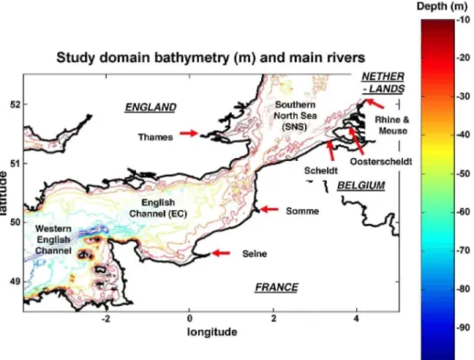
Within the BELCOLOUR domain, the Belgian Coastal Zone (BCZ) is affected by eutrophication problems due to riverine and atmospheric inputs of nutrients modifying the coastal ecosystem equilibria and functioning (Brion et al., 2008; Rousseau et al. 2008b). These mechanisms are obviously influenced by forcing at larger scales than the sole BCZ, and the eutrophication problem is generally addressed from a transboundary and transdisciplinary perspective by marine scientists (Rousseau et al., 2008a). In parallel with ecosystem modelling activities (Lancelot et al., 2008; Lacroix et al., 2007a; Lacroix et al., 2007b) the region of the EC and the SNS [48.5°N-52.5°N, 4°W-5°E] was adopted here. Fig. 1 provides a general view of the domain of interest with bathymetry, borders and the location of main river discharges. When considering the data gaps through the temporal dimension for each sea pixel, the proportion of missing data in the original MERIS and MODIS datasets generally exceeded 75%.

3. Methodology

3.1. Pre-processing

To avoid the production of artefacts in the EOF calculations and subsequent projections, some limitations have to be set on the acceptable spatio-temporal proportion of missing data as in Alvera-Azcárate et al. (2005). Prior to DINEOF treatment, it was chosen to eliminate each image holding less than 5% of the expected data. This reduced the number of exploitable images from 595 to 356 for MERIS and from 1688 to 1291 for MODIS. The same elimination criteria was applied in time, excluding thus from the study all pixels holding less than 5% of valid data through the temporal dimension and producing thus the remaining spatial domain to be considered by the DINEOF analysis. This slightly reduced domain is very similar for both MERIS CHL and TSM, and shows little pixel loss for open sea pixels. Reduction occurred mostly along coasts and in inner parts of some estuaries. After this selection, the MODIS TSM dataset presented a slightly lower proportion of missing data than the MERIS dataset (69% against 73%). Table 1 summarizes the spatio-temporal characteristics of the dataset as submitted to DINEOF analysis, after this pre-processing.

In order to enhance the sensitivity of the DINEOF analysis to the spatio-temporal variations of CHL and TSM data occurring in the lower part of the ranges, the base 10 logarithm of the data was taken instead of direct units. This scale change prior to the analysis reflects the typical statistical distribution of these parameters in nature (Campbell, 1995) and also prevents any reconstructed data to be projected towards negative values of the direct unit scale. The background field is then calculated as the mean value observed in each pixel over all selected images. This field is then subtracted from the dataset in order to provide DINEOF with anomalies around the mean local value measured in base 10 logarithm, enhancing thus the sensitivity of the EOF to coherent variations occurring through domains of very different TSM and CHL concentration ranges that can be found between estuaries, coastal zones and more offshore waters. For SST data, the DINEOF analysis was simply run on temperature anomalies around the background field expressed in direct units.

Table 1 Details of the MERIS and MODIS database used over the channel area (48.5°N-52.5°N 4°W-5°E).

Sensor MERIS MODIS

Period 01/2003-12/2006 06/2002-12/2006

N. images 356 1291

Mean interval (days) 4.1 1.3

Data points 34*10 E6 185*10 E6

Missing data% 73.2 69.0

3.2. DINEOF algorithm

When using only cloud-free images, a very efficient way to synthesize the information contained in a collection of scenes is the use of empirical orthogonal functions (EOFs, also called principal components in other research domains). These functions have some important properties: when only one EOF is used, this EOF is on average the closest to all images, when multiplied for each image by appropriate amplitude. Hence it is the best possible approximation of all images using only one spatial pattern (or EOF) and an amplitude for each image. With two EOFs, it can be shown that no other combination of two patterns can provide a better approximation to all

images than these two. In general the first N EOFs are therefore the best way to summarize the information content of all images if only N patterns can be stored (Beckers and Rixen, 2003). Each image is then replaced by a filtered version in which the basic patterns are linearly combined with specific weight corresponding to each image. When images are sequential in time, the modulation of the contribution of the basic patterns can be interpreted as a time evolution of the spatial patterns and be referred to as temporal modes. The practical calculation of the EOFs can be performed by a singular value decomposition of the data matrix X, of columns of m elements (spatial dimension) and rows of n elements (temporal dimension). To construct the data matrix, each scene is stored as a one-dimensional array and corresponds to a column of the matrix X.

To build each one-dimensional array (unwrapped image), the corresponding original two-dimensional scene is scanned in a column-major order (column by column and pixel by pixel), while only sea pixel values (data or no data) are stored one after another in the new single dimension array. This rearrangement of the scene data carries no spatial information to the DINEOF processing itself, which is in fact only sensitive to covariances between all pixels and does not process information on two-dimensional spatial organisation. Real two-dimensional fields are only reconstructed after DINEOF treatment, based on the spatial domain mask used during pre-processing. The temporal dimension of the data matrix (successive elements within any row of matrix X) is simply built by the compilation of all one-dimensional arrays obtained (as described above) from all scenes for which at least 5 percent of data are present. As described in the pre-processing step (Section 3.1), this elimination of scenes carrying too limited data is made to prevent uncertain reconstructions that could derive from an under-conditioned problem.

The SVD decomposition thus provides 3 matrices as in Eq. (1), giving direct access to the spatial patterns (columns of matrix U), the temporal evolution of these patterns (columns of V) and their overall amplitude (diagonal elements of S).

The amplitudes are generally stored by decreasing importance so that when using not all EOFs but only the first N, we neglect the smallest contributions. In this case, the truncated reconstruction Xr is given in Eq. (2), where

the matrices on the right hand side only contain N columns corresponding to the N EOFs retained.

Retaining only these dominant EOFs filters out some information from the scenes and it is customary to quantify the filtering effect by providing the explained variance when retaining N EOFs. This quantity is generally expressed as a percentage of the total variance (information content) of the original data.

If we had cloud-free images, EOFs could be calculated easily and an approximate representation of each image obtained as a truncated combination of a few EOFs. Hence we can imagine to use this combination of EOFs for points for which we do not have data to interpolate the missing data. Of course there is a circular dependence because the calculation of EOFs requests a set of cloudless images and the interpolation of the missing data requests the knowledge of the EOFs. To solve this problem, an iterative method was implemented in the DINEOF package:

Assuming we know the first EOF, we can estimate the missing data value at any location with this EOF. Once we have this value, the EOF can be recalculated and so on until convergence. Then two EOFs are taken into account with the same approach, before going to a third and so on.

There remains to initialise the iterative process and to decide when to stop adding EOFs to the reconstruction. The initialization of the EOF iterative calculation is done by setting a first guess of zero anomalies in the missing data points of X. This corresponds to starting the iterative process with a data matrix for which all missing data have been replaced by the local mean field value obtained from existing data. From this starting point, the SVD is used to calculate the first guess EOF from the artificially completed dataset. Then, this first guess EOF is used to make an improved prediction of the missing data. This new prediction replaces the first guess made on missing data (local mean field value), and allows thus for a second iterative cycle to start. A second SVD produces a new guess of the EOF, exploited in turn to project new estimates of missing data. This iteration

continues to produce improved missing data and improved EOF until the changes observed in the missing dataset estimates between one iterative cycle and the next one are insignificant. The convergence criterion is reached when the ratio between the root mean square of successive missing data reconstruction and the standard deviation of existing data becomes lower than a threshold value of 1.0e-3. This example of iterative cycle given for a SVD limited to one EOF is then carried out repeatedly but with a SVD decomposition into a growing number of EOFs.

The number of EOFs retained is fixed by a cross validation technique: a few data points are set aside by removing data on some scenes and an rms misfit between the reconstruction and the dataset aside is calculated for each reconstruction. The number of EOFs retained is then naturally the one that leads to the minimal misfit. For more details we refer to Beckers and Rixen (2003) and Alvera-Azcárate et al. (2005).

3.3. Production of complete fields at regular time steps and extraction of multitemporal averages

Once the EOFs are defined, they can be exploited to regenerate full fields at any intermediate moments when no satellite images were acquired, by assuming that a linear interpolation of the temporal modes is a valid estimate of their evolution between the dates at which they were calculated by DINEOF. In the present work, full fields were produced at daily intervals for the whole period. For MODIS, this temporal resolution is generally comparable to the frequency of exploitable images and is probably meaningful, except in some winter periods. For MERIS products over the North Sea, the frequency of input imagery is less than daily and the consequent reconstruction cannot resolve daily dynamics.

Any local or subregional instantaneous reconstruction or multitemporal averages can be reproduced with this approach, according to the objectives of the user. The global methodology presented can thus be exploited for the establishment of weekly or seasonal composites of ocean colour parameters.

3.4. Production of error maps associated to reconstructions

If one considers the DINEOF reconstruction to be the meaningful part of the variability of the input signal and the noise to be the part of the input signal which is not explained by the selected EOFs, simple "observational error" maps could be obtained from the difference between the original incomplete data and the filled data at each time step. However, these observational error maps are as incomplete in space as the input signal and do not correspond to the actual confidence interval around the DINEOF filtered reconstructions as required by users of the filled products.

As demonstrated by Beckers et al. (2006), a very efficient least square fit of EOF amplitudes to an observed subset of data is equivalent to optimal interpolation (OI) if the filtered covariance matrix of DINEOF is used as the ad hoc covariance matrix of OI. This principle is exploited to use the statistically-derived error estimates of an OI analysis as the error fields for DINEOF. Requiring an a priori knowledge of the signal to noise ratio and spatial correlation length of the observational error, this reference solution with full error covariance matrix would also require prohibitive computational resources for inverting the error covariance matrix, losing thus the efficiency advantages of the DINEOF methodology. A first assumption of this approach is to take the variance not retained by the EOF expansion as an estimation of the noise variance µ2

. This is given in Eq. (3), in which

Xr is the reconstructed data matrix, and mp is the number of data present, corresponding to the product of the

spatial and temporal dimensions of the data matrix minus the number of missing points. Another assumption is to consider the error to be spatially uncorrelated, providing thus a simplified and easy to invert error covariance matrix R, as the product of µ2

by the identity matrix I (Eq. (4)).

In reality many remote sensing errors are expected to be spatially correlated (i.e. due to atmospheric correction errors), but in absence of full information on error covariance structures, Beckers et al. (2006) made an

intermediate complexity level assumption by considering that errors are correlated at a prescribed scale L. Their study showed the interest of using a corrected error variance µeff2 (Eq. (5)) instead of µ2 in order to account

efficiently for such spatial correlation of the noise. In Eq. (5), the ratio between the squared correlation length and the product of pixel sizes in longitudinal and latitudinal directions (ΔxΔy) represents the relative density of the data points regarding the correlation length of the error field, while N is the number of modes retained by

DINEOF and mp is the number of data points present.

The value of L is selected so as to minimise the global OI reconstruction error obtained for the same subset of points as used for the cross validation procedure of DINEOF. This ensures that consistent error fields are derived at a reduced calculation cost. The first steps of the error calculation are similar to the steps presented in the following outlier section (Eqs. (6)-(10)). Further details about the error map generation with DINEOF methodology can be found in Beckers et al. (2006).

In the present study, the ocean colour data is processed by DINEOF as the anomaly of the base 10 logarithm of the data around the mean base 10 logarithm field. This introduces a complication for a representation of the associated error maps. When expressed in real units, the confidence interval is asymmetrical and cannot be represented in a single map. Relative error maps calculated in real units as the ratio of error range to

reconstruction value leads to problematic display of the whole range at once, and to extremes values of relative errors due to occasional inconsistent reconstructions. Thus, another relative error representation was chosen: the ratio between the reconstruction error and the standard deviation of the signal captured by the EOFs for the particular pixel. This proved to be the best way to visualize the spatial variability of the reconstruction error within maps covering large ranges of background values. Although not illustrated here, these error maps showed meaningful patterns with respect to the distributions of available input data and to regions exhibiting strong covariances, as described by Beckers et al (2006).

3.5. Detection of outliers from input data

Benefiting from the existing post-processing error map calculation scheme described by Beckers et al. (2006), a methodology was implemented to classify original pixels on a scale expressing the "outlying" character of each local input data. The principle of the outlier calculation is presented shortly hereafter.

The scaled spatial EOFs (defined as the columns of the matrix L) are the set of spatial modes (columns of matrix

U), weighted by the ratio between their associated singular value (diagonal elements of S) and the squared root

of N, the number of modes retained by DINEOF (Eq. (6)).

The matrix Lp is defined by the scaled set of EOFs in which the missing pixels corresponding to an

instantaneous image are set to 0. The covariance matrix between existing data points Cp is calculated by Eq. (7).

The diagonal elements of this observational error covariance matrix are inflated by the corrected observational error variance µeff2 (as defined in Section 3.4, Eq. (5)), to account for the spatial correlation of observational

error. This is presented by Eq. (8) in which I is the identity matrix of dimensions N.

As described in Beckers et al. (2006), the matrix C obtained by Eq. (9) has only to be calculated once for a given image. The correlation length of the observational error can then be tuned at reduced calculation cost to optimize the fitting between the OI derived error values and the subset of residuals obtained at cross validation points used for EOF calculation.

The matrix Esp holds the contributions of all modes to the expected error of all pixels, for a specific scene considered (Eq. (10)). The matrix Esp has a first dimension "i" corresponding to the m pixels of a scene, a second dimension "j" specifying the scene considered in the series of images analysed and a third dimension "k" corresponding to the N modes retained).

A local expected observational error (named here "Deltaij") is calculated for each pixel (index "i") of each scene

(index "j") (Eq. (11)), accounting thus for the spatial variability of the reconstruction error variance. This expected observational error can be considered as the part of the mean misfit which is unexplained by the EOF projection itself.

The outlier value is then calculated, for each input data present, as the absolute value of the ratio between the residual (reconstruction misfit), and the expected observational error Deltaij of the considered pixel.

The resulting outlier coefficient maps can be displayed to visualise how unusual or suspicious are some pixels and patches with respect to the general content of the dataset. They can also be used as a binary mask to eliminate inconsistent input data prior to any analysis, including prior to a second DINEOF treatment. For this, an outlier value of 3 is generally adopted as threshold for this binary distinction between outlier to non-outlier data. For a Gaussian distribution of the misfit, only 0.3% of the data will be larger than 3.

When analysing results over thousands of images, it is desirable to have some indicators which point automatically to periods reflecting intense unusual events for the global field, or towards suspicious image reconstructions linked with unsuitable input dataset (low amount of data with uneven distribution). For the first case, one can exploit simply the temporal deviation of the image mean outlier factor from its global mean as a good indicator for intense unusual events of the global field, or similarly, for any subregion of interest. Concerning the second case, inappropriate input images can be efficiently detected by calculating the

conditioning number of the diagonal covariance matrix Cp or Cpinf (Eqs. (7) and (8)). The condition number of a matrix measures the sensitivity of the solution of a system of linear equations to errors in the data. It gives an indication of the accuracy of the results from matrix inversion and linear equation solution. Tests made on the MODIS TSM reconstruction confirmed that the highest conditioning numbers corresponded to the occasional inconsistent reconstructions obtained from input images characterized both by uneven spatial distribution and very low data presence. In these tests little difference was found between using the covariance matrices Cp or Cpinf. The conditioning number property will be exploited in future work to eliminate the problematic EOF projections prior to the temporal mode interpolation required for regular field reconstruction, thus avoiding degradation of daily field multitemporal averages.

Attempts to improve the outlier binary classification are foreseen by adding a preliminary normalisation of the outlier distributions encountered in each image, and by taking as threshold criteria a certain percentage of the most outlying data. This will allow the user to explore the sensitivity of the outlier classification and to find the ideal cut-off to eliminate most completely the recognized artefacts. Such an approach might prove to be a more appropriate criteria for all parameters, periods, and natures of outlying data, by comparison with using a constant predefined outlier value as threshold.

Further improvements to input image selection in the post-processing could be considered e.g. by using combined selections based on several factors such as conditioning number, missing data proportion and mean outlier value.

4. Results and discussions

4.1. Background fields of MERIS CHL, MERIS TSM, MODIS TSM and SST

The TSM background field from both MERIS and MODIS sensors are very similar (Fig. 2), showing a general positive gradient towards the coasts, an inverse correlation with water depth, and increase around some estuaries such as the Seine. Nevertheless two differences can be noted. First, TSM background values are generally slightly higher for MODIS, this being linked to the very different algorithms used for MODIS and MERIS as described in Section 2.1. Secondly, a much larger coastal buffer zone is eliminated from the MODIS analysis (due to temporal coverage below 5%), while the MERIS dataset includes data very close to shores, for example within the inner part of the Scheldt estuary and in the Oosterschelde.

The MERIS CHL background field (Fig. 2) shows a general positive gradient towards the coasts as they constitute the main source of nutrients for this ecosystem. In this sense, the continental coast influence appears more pronounced than the English one as the concentrations of the dissolved inorganic nutrient originating from continental river discharges (Lacroix et al., 2007a) are more important than the English ones because of the much larger extent of their watersheds.

The MODIS SST background field (Fig. 2) shows a general latitudinal gradient, with highest temperature found in the bay of the Mont-Saint-Michel and along the coast of Cotentin (2°W, 49°N) and in the bay of the Seine estuary (0°E, 49.5°N), while lowest temperatures are found close to the English coasts in the SNS.

Fig. 2. Background fields obtained for MERIS TSM, MERIS CHL, MODIS TSM and MODIS SST.

4.2. 3 dominants EOFs retained for MERIS TSM and comparison with MODIS TSM

The MERIS TSM signal was optimally synthesised by DINEOF when using 18 modes (minimising the global error estimator), accounting for a total of 97.2% of the input signal variability. The 3 principal modes are illustrated in Fig. 3, together with the corresponding parameter representing the variability of the original signal explained by each EOF. The first mode of MERIS TSM accounts for about 40% of the input signal variability and is clearly a seasonal signal, being positive in winter and negative in summer: it shows a general winter increase of surface TSM in most of the domain but particularly in shallow areas, and the opposite in summer. This seasonality of TSM is known to be linked with the seasonal cycle of average wind intensities over the area (Fig. 1.4 of Ruddick and Lacroix, 2008). The contribution of this EOF in the western EC is opposite, with increasing contribution in summer and decreasing contribution in winter, relative to the background field. This summer increase can be linked to an increase of phytoplankton. The second mode accounts for 12% of the signal variability and represents, relatively to the previously explained signal, general contributions to local reduction of TSM in the SNS, in the south-east coasts of England and along the French coast ranging from Normandy (1°W, 49.5°N) till the strait of Dover (1.5°E, 50.8°N); to the exception of the fall season. This second mode describes contributions towards an increase of TSM in the western and central parts of the EC in summer, relatively to the dynamics explained by the previous mode. Still accounting for 8% of the signal variability, the third mode shows complex spatio-temporal modulations, and the difficulty of interpreting of the modes in terms

of in situ dynamics increases as we look at the further retained modes. These further modes have progressively lower weight in the reconstruction of the complete signal and should rather be seen as corrections ( sometimes partly compensating each other), pulling the reconstructed signal towards the finer significant variations of the input signal.

Fig. 3. 3 principal EOFs obtained for MERIS TSM (spatial modes: spatial modulation around the background

field due to each EOF; temporal modes: temporal variation of the contribution of each mode for the period 01/2003-06/2005).

With about 3 times more images, a more consistent dynamics could be detected from the MODIS TSM dataset compared to the MERIS signal as a similar total explained variability (97.5%) was optimally synthesised into a lower number of modes (14), showing a less noisy appearance mainly in the first modes. Furthermore, the higher variance explained by the upper level modes of MODIS (mode 2 and above) indicates that these EOFs are carrying more consistent information on the dynamics then the corresponding MERIS modes. For MODIS, the first mode describes a general seasonal signal with an increase of TSM in winter and reduction in summer in most of the domain. Comparatively to the MERIS first mode, the increase is more uniform in the EC and clearly less intense in the SNS.

Some important spikes can be observed in the spatial modes of MODIS TSM and SST (Figs. 4 and 6). Many of these spikes can be seen in the same location in various modes, indicating that they result from bad single point data in some images, probably outliers. These artefacts are propagated in the reconstructions and unrealistic spikes appear regularly at the same locations of filled images. Further work will exploit a double DINEOF loop analysis to eliminate this problem. The first DINEOF loop will be devoted only to point out and eliminate outliers as described in Section 3.5, while the second loop should produce smoother modes and reconstructions exempt from these spikes and artefacts. Although outliers problems are also well identified in MERIS TSM and CHL input data (Section 4.4), no spikes are observed in their spatial modes.

Fig. 4. 3 principal EOFs obtained for MODIS TSM (spatial modes: spatial modulation around the background

field due to each EOF; temporal modes: temporal variation of the contribution of each mode for the period 01/2003-12/2005).

Fig. 5. 3 principal EOFs obtained for MERIS CHL (spatial modes: spatial modulation around the background

field due to each EOF; temporal modes: temporal variation of the contribution of each mode for the period 01/2003-06/2005).

Fig. 6. 3 principal EOFs obtained for MODIS SST (spatial modes: spatial modulation around the background

field due to each EOF; temporal modes: temporal variation of the contribution of each mode for the period 06/2002-12/2006).

4.3. Background fields and 3 dominants EOFs retained for MERIS CHL

For MERIS CHL, a combination of only 8 modes was retained by DINEOF for optimal reconstruction. The 3 principal modes are illustrated in Fig. 5. A total of 93.5% of the variability of the original signal was explained by this EOF synthesis. Although still high, this total variability explained is slightly lower than for TSM perhaps because of the greater complexity of factors affecting phytoplankton dynamics: advection and mixing but also biotic processes (growth as affected by nutrients, light and temperature, grazing, competition, self-shading). The greater algorithm uncertainties for remote sensing of CHL in turbid waters may be a second reason. The temporal evolution of CHL modes are similarly more complex than for TSM modes, with many intense shifts. Hence, interpretation of EOFs in terms of in situ dynamics is more complicated than for TSM case and the permanence of sign (positive or negative) of the EOF temporal mode during some periods is more easily interpreted and meaningful than high frequency fluctuations.

The first CHL mode accounts for 31% of the input signal variability and shows a general concentration increase over the domain, particularly pronounced off the southern English coast. The sign of this contribution tends to remain positive for long periods during the spring and during late autumn or early winter, reflecting the main signal variability: the spring and autumn bloom events occurring in areas corresponding to low average

concentrations on the background field map. The second CHL mode accounts also for an important value of the input signal variability (20%). It describes patterns of concentration increases and decreases that are opposite and complementary in space with those presented by the first mode. Still accounting for 12% of the input signal variability, the third mode describes spatially distinct but coherent contributions to CHL concentration variations occurring off the Dutch coast on one side and on the other side in the middle of the western EC, with the longest periods of positive peaks occurring mainly in spring-early summer.

In regard to the complex phytoplankton dynamics of the area, the interpretation of the second and third CHL modes dynamics are beyond the objectives of this methodological study, but for future investigations, the following contributions to the analyzed signal should be considered.

Some local blooms of Karenia mikimotoi may occur in the seasonally stratified region extending from the central western EC to the coast of Cornwall (4.5°W, 50°N) as described by Le Corre et al. (1993) and Rodriguez et al. (2000). Vanhoutte-Brunier et al. (2008) described, with support of SeaWiFS imagery, the early and very intense monospecific Karenia bloom that occurred in spring-summer 2003. They also suggested to study the effect of inter-annual variability of fresh water intrusions from the Atlantic shelf (Kelly-Gerreyn et al., 2007) on Karenia bloom dynamics. The dynamic of other phytoplankton groups at larger scale should also be considered to attempt a deeper analysis of the reconstructed CHL signal. Indeed, with general transport of Atlantic water entering the western EC, phytoplankton biomasses originating from the nearby continental margin in the Gulf of Biscay or from the Celtic sea can be advected to the western side of the Channel (Garcia-Soto et al., 1995), and be observed in the western part of the area studied here, either still in a growing phase or as a decaying bloom (B. Delille, personal communication).

4.4. Background fields and 3 dominants EOFs retained for MODIS SST

The MODIS SST dataset could be synthesised into 13 modes explaining 98% of the input signal variability, of which 67% just by the first mode. The 3 principal modes are illustrated on Fig. 6. The first mode confirms the seasonal cycle of solar radiation heating as the main driving factor of temperature dynamics in the study area. It illustrates a coherent temperature fluctuation for the whole domain, with an amplitude inversely related to water depth. Under the form of a general gradient from the western EC to the SNS, the second mode accounts for 7% of the signal variability and describes a seasonal modulation with a summer contribution to local increase of temperature in the SNS and decrease in the western Channel, relatively to the first mode, and the opposite trend in winter.

Fig. 7. Illustration of original fields, outliers and reconstructions maps for: MERIS TSM on 13/04/03 with

probable undetected haze, MERIS CHL on 18/10/03 with clear outliers at cloud edges, MODIS SST on the 17/08/02 with numerous outliers spread throughout a large clouded area.

4.5. illustration of original and filled images with associated outlier coefficient

As described in Section 3.5, outlier maps can now be produced in association with each input image analysed by DINEOF. Outlier maps represent, for each pixel, the ratio between the observational error and the expected error. Conventionally, any outlying coefficient above a value of 3 would indicate an outlying pixel in the input

image. Clear detections of outliers have been observed during the various analyses. Typical situations for which artefacts in original images were detected as higher outlier values are illustrated in Fig. 7, with probable haze in the MERIS TSM image of 13/04/03, with some clear cloud edges and suspect noisy low values frequently affecting MERIS CHL images, as on the 18/10/03, and with numerous outliers spread throughout a large clouded area in the MODIS SST image of the 17/08/02. This MODIS SST image illustrates well a case where a single pass DINEOF reconstruction cannot filter the outlying input data but is rather strongly influenced by problematic pixels. A large zone of isolated and spread pixels of extreme low values is found in the middle of a large clouded area (Pison and Nechad, 2006). Well spotted as outliers, these values are numerous and consistent in space, pulling the reconstructed field to display an inconsistent very low temperature zone (12 °C) in a summer field ranging from 16 to 20 °C.

For the scene of 16/09/03 (Fig. 8), MODIS TSM and MODIS SST fields are both affected by problems of cloud edge with similar shapes in the central EC, and by the same contrails in the western EC. It is interesting to note that the intensity of the outlying signals is not exactly similar. Although clearly affecting both regions and TSM and SST input images, some part of contrails are well detected in the TSM outliers, while others are better spotted by the SST outlier field. Thus, there could be an advantage to exploit jointly outlier detection information derived from several parameters to improve the overall data quality of each type of input data. This will be especially relevant for undetected clouds affecting both TSM and SST products.

Despite the limited number of EOFs retained, the sensitivity of DINEOF methodology to the presence of outliers can be explained as follows. The limited series of modes selected by DINEOF is that which allows a

reconstruction of original cross validation data with a minimal global reconstruction error. Therefore, this combination of EOFs is the most sensitive to the significant coherent variational modes that are present in the incomplete dataset. As such, it is also the combination of modes that points most efficiently towards the original signal variations which appear to be incoherent with the global dataset. This incoherence is pointed out by an excessive reconstruction error observed when compared with the statistically expected reconstruction error. Fig. 8. Illustration of original fields, outliers and reconstructions for MODIS TSM and SST on the 16/09/03,

showing slightly variable but complementary signatures of contrails and cloud edges artefacts in their outlier fields.

4.6. Validation of reconstruction (MERIS TSM and CHL) 4.6.1. Objectives and constraints of validation method and cases

In the present work we have adopted a modest validation procedure by adding typical sized clouds. This is a first standard approach in DINEOF processing which has the advantage of being representative of the real data gaps (large clouds) frequently occurring in the North Sea area. This validation procedure aims to demonstrate and explain how the reconstruction quality is related to the variability of the target parameters. The objective of our validation work is to produce a first sound comparison of reconstruction quality through extremes environmental conditions characterized by most homogeneous areas to highest gradient area, and to allow this comparison for the two parameters CHL and TSM. For the current work this was already quite challenging because of the undersampling of natural variability and gappiness typical of the input dataset, which left few suitable dates for demonstrating comparative reconstruction. To compare with reference analysis for which all existing data are used, specific DINEOF analyses were carried out on slightly modified inputs: existing data being removed under two identical artificial clouds for 3 images of the series. Data were removed below 'false clouds' appropriately placed: a homogeneous region (the central part of the EC, referred to hereafter as cloud 1) and a region usually displaying important spatial gradient (the Belgian coastal region, referred to as cloud 2). The 3 images processed were chosen in relatively cloud free weeks so that the typical spatial patterns observed for the other days of these periods could be theoretically captured by the EOFs.

For both TSM and CHL, the dates chosen were the 16/04/03, 27/10/ 03 and 16/07/06.

Future researches will be oriented towards a more systematic validation methodology and, for example, plan to look at new satellite data sources with much higher sampling frequency (Neukermans et al, 2009) to facilitate.

4.6.2. Results of reconstruction quality estimates

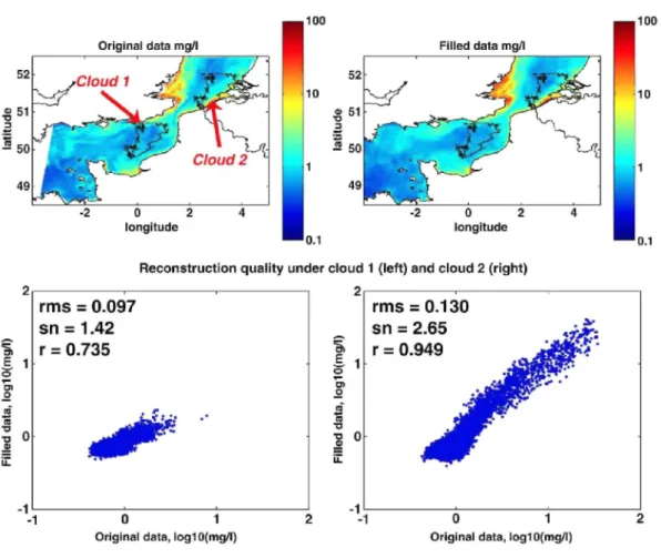
The estimation of the reconstruction quality obtained under these artificial clouds on the 16/07/2006 is illustrated in Fig. 9 for TSM and Fig. 10 for CHL. Original, unused data are displayed below the clouds delimited by black contour lines, for visual comparison with the reconstructed fields obtained. The quality of the reconstruction is estimated by statistical parameters calculated from original unused data and reconstructed data obtained below the artificial clouds, as indicated on these figures. These parameters are root mean square of the reconstruction error (rms), signal to noise ratio for the reconstructed datasets (sn) and correlation coefficient between unused and reconstructed data (r).

For both TSM and CHL, Table 2 summarizes the ranges of r, sn, and rms error obtained in this validation of the reconstruction below artificial clouds.

Table 2 Ranges of correlation coefficient (r), signal to noise ratio (sn) and root mean square error (rms)

obtained in the validation of the TSM and CHL DINEOF reconstructions below artificial clouds (cloud 1 : homogeneous region; cloud 2: high gradient region) for 3 different images.

TSM CHL

Min Max Min Max

Cloud 1 r 0.47 0.83 0.25 0.58 sn 1.04 1.67 0.88 1.15 rms 0.10 0.11 0.09 0.19 Cloud 2 r 0.87 0.95 0.12 0.70 sn 1.94 2.65 0.99 1.27 rms 0.13 0.15 0.17 0.29

4.6.3. Discussion of reconstruction quality estimates

Minimal signal to noise ratio are of the order of 1 for both parameters, meaning that the importance of the error is, in the worse situations, comparable to the signal. This is generally found in situations where the signal is itself of low intensity and uniform across the clouded regions, rather than to be due to larger absolute reconstruction errors.

With a wider range of input values below the cloud number 2, the reconstruction quality parameters sn and r are most of the time higher, both for TSM and CHL. The rms values are also systematically higher under cloud 2, but less than proportionally with the signal variability as shown by the signal to noise ratio. These results suggest a better response of EOFs to the reproduction of the signal observed in regions of high gradients and high variability, relatively to regions of rather more homogeneous values.

In the Belgian coastal zone, reconstructions are consistently better for TSM for the 3 selected test days, with sn ranging from 1.9 to 2.7 while it was limited to a maximum of 1.27 for CHL. Correlation coefficient was also higher for TSM (from 0.87 till 0.95) than for CHL (0.12 till 0.7). Generally, the lower quality results obtained for CHL illustrate the greater complexity of phytoplankton spatio-temporal variations and/or retrieval uncertainties.

The range of reconstruction quality was estimated from worse to best situations, as well as within the selected images, between relatively homogeneous zones as well as regions of strong gradient and results are encouraging. The quality of the reconstruction depends on the coherence/ repeatability of the signal being analyzed, which is itself a representation of natural processes but with discrete sampling and measurement errors. Thus, low reconstruction quality estimates can occur when:

1. The natural processes show low coherency, e.g. phytoplankton blooms which may occur for different subregions in a decoupled fashion with different timing, or with low coherency in the shape of successive bloom fronts within a same subregion.

2. The natural processes are undersampled, both in time and/or in space. In the present study case, level of data gaps are significant (order of 70%), underlying the difficulty of the reconstruction challenge addressed. This is seen particularly for the reconstruction of MERIS CHL data where the proportion of missing data is higher than for MODIS TSM. This can also specifically occur for original scenes for which a little amount of data are present but spread unevenly, leading to an under-conditioned EOF projection problem.

3. The natural processes are poorly represented in some input scenes,. This can occur for scenes for which important proportion of erroneous data (outliers) remain because of processing uncertainties, e.g. undetected cloud-edge pixels. In this respect the DINEOF reconstruction quality estimate can provide useful information on weaknesses in the satellite data processing.

Future studies, which would not have to produce comparable quality estimator for both TSM and CHL on same dates and locations, might complement the validation by focusing on other regions, possibly with different approaches such as using numerous smaller and evenly spread false clouds checks, or as analysing validation results as function of the temporal variability of the input signal at specific pixels.

4.7. Daily regular reconstructions, multitemporal climatologies and time series extraction at reference stations

For all analysed parameters (MERIS TSM and CHL, MODIS TSM and SST), daily reconstructions were produced by EOF projection using interpolated temporal amplitudes, over the 4 year period of the input dataset. This daily regular reconstruction step is made as a post-processing of the DINEOF methodology and the validation presented in Section 4.6 only concerns DINEOF direct reconstructions of existing incomplete satellite scenes. For some relatively cloud-free periods between spring and late fall, the temporal dynamics of daily MODIS reconstructions can be comparable to the frequency and availability of input data. As an illustration of the fine TSM dynamics that can be reconstructed from MODIS for such periods, an animation showing daily reconstruction at 12h00 UTC can be downloaded as complementary information from (http://

modb.oce.ulg.ac.be/projects/2/RECOLOUR_products) and from the present journal web site (Video 1). However, occasional local spikes are observed in daily reconstructions, as occasional incoherent fields. This latter problem occurs when EOF projection is made from unsuitable input data leading to an under-conditioned

problem. A mathematical problem is considered well conditioned if the sensitivity of the solution to

perturbations on the data remains acceptably low, as described by Toumazou and Creteaux (2001). At this stage of the research into optical products, users of the present research reconstructed products are advised to use the more robust weekly averages as the highest temporal resolution of the analysed colour product signal.

Weekly and monthly averaged fields were produced from reconstructed daily fields for MERIS TSM and CHL products, and for MODIS TSM and SST products. These new climatologies have the advantage that missing data were replaced by estimates resulting not only from information provided by the existing parts of the scenes considered but also from the data covariances detected throughout the whole database. For this reason, the new monthly and weekly climatologies produced are supposed to be less biased by the spatio-temporal heterogeneous distribution of clouds then classical climatologies would be. While detailed quantification of differences is left for further work, a simple comparison of both methodologies shows the practical advantage of the DINEOF approach over classical averaging, for which results are contaminated by discontinuity patterns and lack of coverage (Fig. 11).

Fig. 11. Comparison of weekly climatological fields obtained from daily DINEOF reconstructions (left) and

from classical averaging of present data (right); examples of MERIS CHL (top; in April 2003) and MODIS TSM (bottom; in august 2002).

As illustration of the interest of studying seasonal dynamics from reconstructed continuous time series, weekly averaged MERIS TSM and CHL reconstructed signals were extracted from one pixel corresponding to a turbid water station near the Scheldt Estuary mouth (51.47°N; 3.23°E, identified by a spot on Fig. 11). These

reconstructed averages are plotted from January 2003 till June 2004 (Fig. 12), in regard to the weekly averages calculated from the existing original data extracted in the same pixel from the instantaneous images.

The fact that no data are available in this pixel for several original scenes doesn't mean that DINEOF

reconstructed values will only be influenced by the other data available for that pixel. When producing the daily reconstruction in this missing spot, DINEOF can be affected by the presence of higher or lower TSM

concentrations data existing in other locations for which strong covariances with our missing spot were detected by the EOFs. So, for several days of a week, the instantaneous values reconstructed by DINEOF in the missing spot can happen to be much higher (or lower) than the value sensed directly by the satellite in one moment of

this week. In consequence, it is absolutely possible that the weekly average value of the DINEOF reconstruction obtained in one pixel will be well different (higher or lower) than one or few existing original instantaneous data in that pixel. This is justifying what is for instance happening in the end winter/beginning of spring for TSM in Fig. 12.

Continuous time series are far more convenient for analysis of environmental dynamics then sparse

instantaneous data and show well the strong seasonal TSM dynamics and the onset of the spring CHL bloom. These reconstructed averages show also the unusually intense spring bloom event observed in the Scheldt plume in 2003 and described in Borges et al. (2008).

Any reconstructed product extracted from the study domain can be obtained by contacting the authors or by posting a request at (http://www.mumm.ac.be/BELCOLOUR/EN/sendmail.php).

Fig. 12. Weekly averaged time series of MERIS TSM and CHL calculated from daily DINEOF daily

reconstructions in a pixel of the Scheldt Estuary mouth turbid waters (51.47°N; 3.23°E), versus original existing data extracted from the same pixel.

4.8. Perspectives for elimination of artefacts

Future work will involve successive DINEOF runs as an attempt to eliminate the spikes captured by the EOFs and reconstructions as consequence of outlying input data. According to preliminary tests, inconsistent EOF projections should be eliminated by the use of the conditioning number of the field covariance matrix, a criterion defining the sensitivity of the EOF projection to possible uncertainties on the input data. Thus, new solutions are in the testing phase for improving further the quality of instantaneous reconstructions as of multitemporal averaged fields.

5. Conclusions

This study demonstrates successful applications of the parameter free DINEOF method to the reconstruction of 4 years of satellite TSM, CHL, and SST data in the EC and the SNS. For the CHL and TSM products, a significant part of the variability of the input signal (93.5 to 97.5%) could be synthesized into a limited number of modes (8 to 18), allowing optimal reconstructions of the complete fields, even with a very high proportion of missing data (70%).

Optimal reconstructions were obtained by DINEOF when synthe-sising the original signal into 8 modes for MERIS CHL and into 18 modes for MERIS TSM. The variability of these original signals explained by the EOF synthesis reached 93.5% for CHL and 97.2% for TSM. For the MODIS TSM dataset, 97.5% of the original variability of the signal could be synthesised into 14 modes, but with less variability explained by the first mode comparatively to MERIS TSM, revealing a seasonal signal better captured and described by two modes instead

of one. This results probably from the higher frequency of image acquisition and from the lower global

proportion of missing data of the MODIS dataset. The MODIS SST dataset could be synthesised into 13 modes explaining 98% of the input signal variability, of which 67% only by the first mode, as expected due to the strong seasonal pattern of the SST dynamics for this area.

For MERIS TSM, the reconstruction quality was evaluated for 3 dates below 2 artificial clouds and proved very encouraging with correlation coefficients ranging from 0.45 to 0.95, and signal to noise ratio between 1 and 2.7. Reconstruction quality of CHL was lower with correlation coefficients ranging from 0.12 to 0.70, and signal to noise ratio comprised between 0.88 and 1.27.

Daily reconstructions were produced by interpolation of the temporal mode coefficients. Weekly and monthly averaged fields were produced from these daily reconstructions, underlying the interest of the method for the establishment of multitemporal composites. These are expected to be less biased than classically averaged products, which are affected by the heterogeneity of cloud coverage. Any subregional or local multitemporal averages can be reproduced with the described DINEOF approach, according to user needs.

The regular and full gridded weekly averaged fields are useful for forcing or validation of ecosystem models. For instance, the weekly averaged TSM fields produced here are being exploited to test the impact of light

attenuation on phytoplankton blooms.

Error maps associated with every reconstruction were produced according to Beckers et al. (2006). An outlier detection method was implemented on the basis of this error calculation scheme. It produces, for every input image, a map of coefficients representing the absolute value of the ratio between the observational error (difference between original and reconstructed fields) and the expected error of the reconstructed field itself. Several original input data can be identified as suspect by the users, as illustrated for CHL in Ruddick et al. (2008b). After the present analysis, several input data appeared clearly as higher values in the outlier maps (undetected cloud edges, haze areas, contrails, and cloud shadows). The method is also efficient in detecting events considered as unusual with respect to the available image database. The structures observed in the outlier maps are generally very distinct from normal data, although the classical threshold criteria of 3 is not always reached for all of the suspect data (i.e. only some part of the clearly visible contrails are detected as outliers). Future improvement of the outlier classification could be an automatic adaptation of the outlier threshold setting based on a normalisation of the outlier value distribution of each image. The combination of outlier signatures associated with the various parameters (CHL/SST/TSM) produced from a same scene is another promising direction for improving outlier detection.

With the production of outlier maps, the DINEOF data reconstruction technique becomes a very efficient tool for automatically analysing large databases. It opens the way to potential applications in the processing and quality control of optical remote sensing data, adding statistical information to the conventional spectral processing. Supplementary materials related to this article can be found online at doi:10.1016/j.seares.2010.08.002.

Acknowledgements

This work was realized in the context of the RECOLOUR (REconstruction of COLOUR scenes - SR/00/111), and BELCOLOUR-2 (SR/00/ 104) projects funded by the Belgian Science Policy (BELSPO) in the frame of the Research Program For Earth Observation "STEREO 11."

The MERIS products were supplied by the European Space Agency under Envisat A01D698. NASA/Goddard Space Flight Centre is thanked for MODIS data.

This is MARE publication.

References

Allen, J.I., Blackford, J., Holt, J., Proctor, R, Ashworth, M., Siddorn, J., 2001. A highly spatially resolved ecosystem model for the North West European Continental Shelf. Sarsia 86, 423-440.

Alvera-Azcárate, A., Barth, A., Rixen, M., Beckers, J.-M., 2005. Reconstruction of incomplete oceanographic data sets using Empirical Orthogonal Functions. Application to the Adriatic Sea surface temperature. Ocean Model. 9, 325-346.