SENSOR NETWORK DESIGN USING GENETIC ALGORITHM
C. Gerkens, G. Heyen
Laboratoire d’Analyse et de Synthèse des Systèmes Chimiques University of Liège, Sart-Tilman B6a, B-4000 Liège (Belgium)
Tel: +32 4 366 35 23 fax: +32 4 366 35 25 Email: [email protected]
Abstract
A systematic method to design optimal redundant sensor networks applying data validation theory is described. Sensor networks are optimised thanks to a genetic algorithm. The design objective is to estimate the process key variables within a required accuracy. The solution time is reduced by means of two parallelisation techniques both using the MPI library: the global parallelisation method and the distributed genetic algorithm method. Results are presented for an ammonia synthesis loop.
Keywords: design, sensor network, genetic algorithm, data validation, parallelisation, MPI.
1. INTRODUCTION
Chemical processes must be monitored correctly to ensure that all safety and environmental constraints are verified and that the quality required for products is achieved. This requires a suitable measurement system. Redundancy allows to detect and correct some measurement errors, and reduces the uncertainty of the estimates.
Moreover some variables of the process (such as compressor’s efficiency, reactives’s conversion…) can not be obtained directly by mean of a sensor. Data validation techniques allow to solve these problems by exploiting a model of the process and measurements’ redundancy. Indeed each measurement is corrected as little as possible to satisfy balances and non-measured variables are estimated. Moreover a posteriori accuracies are calculated for all variables. As the state variables for streams are enthalpy, pressure and partial molar flow rates, link equations relating measurements and state variables have to be added to the model. Moreover, link equations expressing key parameters (such as efficiencies, heat transfert coefficients) as functions of state variables and measurements have also to be added.
The efficiency of this method depends of the sensor network that is used: indeed, according to the number, the position and the accuracy of the different sensors installed, process variables can be estimated more or less accurately. The problem is therefore to find out the cheapest redundant sensor network able to estimate process key parameters within a prescribed accuracy.
Until now only few studies have been carried out in this field: thanks to a graph oriented method, Madron (Madron, 1972) solved the linear mass balance case. Some years after Bagajewicz (Bagajewicz, 1997) analysed the problem for mass balance networks where all constraint equations were linear.
The goal of our research is to solve broader problems including energy balances and non-linear constraint equations.
In our approach all state variables are candidates for measurement. The unmeasured ones have a very large standard deviation. The Lagrange formulation of the data validation problem is thus:
( ) ( ) ( ) min ' ' 2 , T T L X X W X X A X D X λ λ = − − + + (1.1) where
- X is the array of process variables - X’ is the set of measurements
- W is the weight matrix (i.e. the inverse of the measurement covariance matrix)
- A is the Jacobian matrix of the linearised model (constant).
Solving this equation for stationarity conditions:
1 1 ' ' 0 T X W A WX WX M D D A λ − − = = − − (1.2)
The elements of M-1 are obtained using a LU factorisation of M. To take advantage of the sparsity of the sensitivity matrix; we used the Belsim’s sparse matrix code. A singular matrix M corresponds to a sensor network that does not allow to estimate all process variables.
The variances of validated values of variables can be estimated if the measurements variances are known (Heyen et al., 1996):
( )
(
( )
)
2 1 , 1 var var ' m i j i j j M X X − = =∑
(1.3)The major contributions to the objective function of our optimisation problem are the annualised cost of the sensor network and a function of sensor accuracies. The objective function is optimised thanks to a genetic algorithm.
As the time required to obtain a solution is quite long, the algorithm has been parallelised by means of the global parallelisation method and distributed genetic algorithms.
2. GENETIC ALGORITHM DESCRIPTION The proposed method is carried out in five steps that are described in this section. An example of application is presented in the next section.
2.1.FORMULATION OF THE VALIDATION MODEL AND MODEL LINEARISATION
The coefficients of the model matrix A are automatically generated from a Vali3 data validation model (Belsim 2001). The model is build by drawing unit operations in a process flow diagram and by linking them by means of material or energy streams. For material streams, a thermodynamic model has to be chosen from the list proposed. The Vali3 software writes automatically the link equations for standard measurements types but link equations have to be created for non-standard unmeasured variables such as reaction conversion. The variables whose values are known in the operating conditions are specified. The number of specified values has to be at least equal to the degree of freedom of the model. As overspecifications bring additional information and that data validation gives a “least square” solution, overspecifications are allowed.
The problem is then solved thanks to the Lagrange multiplier method or a SQP solver. When the solution is obtained, a report file is generated containing the value of all variables and their accuracy, the linearised equations of the model and the non-zero coefficient of the Jacobian matrix. This report is then read by the sensor optimisation program. If the sensor network have to be available for several operating points, a report is generated for each of them.
2.2.SPECIFICATION OF SENSOR DATABASE, PRECISION AND SENSOR REQUIREMENTS
The program needs three files besides the Vali3 report:
THE SENSOR DATABASE
This file contains for each sensor: - the sensor name;
- the sensor annualised cost (operating, purchase cost and installation costs);
- the sensor accuracy
σ
, which is related to the measured values :'
a b X
σ= + (2.1) - the type of variable that can be measured by the
sensor.
THE PRECISION REQUIREMENTS
Key variables of the process have to be known quite precisely. A file is prepared, listing all key variables and their required accuracy target (maximum standard deviation). At each generation of the optimisation algorithm it is checked whether the key variables accuracies are acceptable or not.
THE SENSOR REQUIREMENTS
Sometimes, the plant configuration is such that it seems impossible or obligatory to put a sensor on a determined place, or some sensors are already installed on the plant and even if they are not located optimally they can’t be displaced.
In such cases, sensors that must be installed in some location, or that are to be excluded are listed in a file. 2.3.VERIFICATION OF PROBLEM FEASABILITY
At this step, the programme starts identifying by looking for all possible sensors. This sensor network is the most expensive one (Cmax) that can be found by
the algorithm. Afterwards it checks whether there exists a solution to the problem by solving the linearised data validation problem for the sensors network it has just found. If a variable is measured by more than one sensor, the variance of the most accurate one is taken into account.
The two following conditions have to be met: - the sensitivity matrix M of the problem must be
non-singular. If this condition is not met the programme stops.
- the variances of the process key variables must be acceptable. If this second condition is not met, the programme may continue but a penalty is added to the objective function. There are different ways to met this condition: adding more precise sensors, adding sensors that can measure other type of variables, adding more extra variables with their link equations so that more variables can be measured.
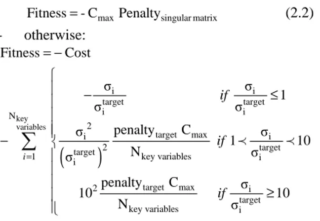
2.4.OPTIMISATION OF THE MEASUREMENT SYSTEM If a solution exists for the problem, the search for the optimal solution can begin. The objective function to be maximise (fitness) is evaluated this way:
max singular matrix Fitness=- C Penalty (2.2) - otherwise:
(
)
key variables i i target target i i N 2 target max i i 2 targettarget key variables
1 i i target max 2 i target key variables i Fitness Cost σ σ 1 σ σ penalty C σ σ 1 10 N σ σ penalty C σ 10 10 N σ i if if if = = − − ≤ − ≥
∑
≺ ≺ (2.3) If the sensor network has to optimised for several operating points, the objective function is estimated by the following formula:functioning points N j functioning points j=1
Fitness= fitness −N −1Cost
∑
(2.4)The objective function is multimodal in most of the cases. Moreover the number of binary variables of the optimisation problem is large and the problem is not derivable. That is why a genetic algorithm (Goldberg, 1996) is used to perform the optimisation. The implementation adopted is base on the code developed by Carroll (Carroll, 1998). This code uses the natural selection mechanisms of tournament selection (random pairs are chosen thanks to a shuffling technique), single-point or uniform crossover and jump mutation.
The sensor network to be optimised is expressed as a character string called chromosome. Characters are binary decisions called genes and represent the presence of a sensor at a given location in the network.
The first population is generated randomly by biasing the initial chromosome in which all the possible sensors are chosen: a high probability of selection of 80 % is fixed for each sensor to be sure the number of chosen sensors is at least equal to the number of degrees of freedom. It appears that this parameter is not critical.
The others parameters of the algorithm are fixed as follow:
- the size of the population is most of the time fixed to 20 chromosomes;
- the reproduction probability: 50%; - the crossover probability: 50 %;
- the mutation probability after reproduction or crossover: 1%.
At each generation, the objective function is evaluated for each chromosome and the best individual is kept. If the best individual stays unchanged after a specified number of generations, it is considered as the solution of the problem.
2.5.REPORT GENERATION
Once the optimal sensor network is obtained, the programme prepares a report containing the list of the sensors chosen with their position, the accuracy predicted for all process variables and a comparison between the obtained and the target accuracies for the key variables.
3. A CASE STUDY: NH3 SYNTHESIS LOOP In this section we will show the results obtained for an ammonia synthesis loop. That process involved 14 units (one two-stage compressor with two intercoolers, one recycle mixer, one recycle compressor, one reactor preheater, one ammonia converter, one waste heat boiler, one waste cooled condenser, one ammonia cooled condenser, one liquid-vapour separator, one purge divider and one flash drum for expanded ammonia condensate), 19 process streams (composed of ammonia, nitrogen hydrogen, argon and methane), 10 utility streams and 3 mechanical streams. The model comprises 224 variables and 177 constraint equations. Target accuracies are specified for 58 key parameters. The sensor database comprises 15 sensor types: 3 temperature sensors, 2 pressure gauges, 2 chromatographs, 1 poly-analyser, 1 oxygen sensor, 4 mass flowmeters and 1 molar flowmeter.
The maximum number of sensors that can be installed is 117. That means that the solution space involves 2117=1.7 1035 solutions. The total cost of this network is 8600 units.
In the case of the obtention of a redundant sensor network, the algorithm found a solution after 640 generations or 12800 objective function evaluations for a stop criterion of 200 generations. The evolution of the objective function is represented on figure 1. The time required to obtain that solution was about 10 minutes on a Pentium II (330 MHz) computer. The sensor network obtained costs 1580 units and consists of 39 measurement tools: 1 chromatograph,
Evolution of the objective function
-9000 -8000 -7000 -6000 -5000 -4000 -3000 -2000 -1000 0 0 100 200 300 400 500 600 700 Generations O b je c ti v e f u n c ti o n
Figure 1: ammonia synthesis loop: evolution of the objective function in the case of redundant sensor network
7 mass flowmeters, 20 temperature sensors, and 11 pressure gauges. This sensor network is presented on figure 2.
If it is desired that the sensor network stays observable in the case of one sensor failure, the measurement system is obtained after 366 generations for a stop criterion of 200 generations. The time required to obtain that solution was about 8
hours and 15 minutes on a Pentium II (330 MHz) computer. The sensor network obtained costs 3900 units and consists of 67 measurement tools: 2 chromatographs, 13 mass flowmeters, 31 temperature sensors and 21 pressure gauges. This sensor network is presented on figure 3.
Figure 2: validable measurement network for an ammonia synthesis loop
4. PARALLELISATION
As the solution time is quite important, larger problem couldn’t be taken into consideration without parallelising the code. Indeed, parallelisation methods allow to reduce the solution time because they share the computing work between several processors. Parallelisation techniques are compared using the notion of efficiency:
Speed up Efficiency
Number of active processors
= (4.1)
Time for 1 processor Speed up
Time for n processors
= (4.2)
The algorithm was parallelised applying MPI routines (Gropp et al, 1999) to the global parallelisation method and the distributed genetic algorithms. All calculations were carried out on a cluster of identical Apple Power Mac bi-processors.
4.1.GLOBAL PARALLELISATION
This method consists of carrying out in parallel the evaluation of chromosomes’ fitness. In the case of our algorithm, the time limiting step is the evaluation of the objective function. Indeed, the size of the sensitivity matrix to be inverted is equal to the sum of the number of variables and the number of equations of the problem. The solution time of the algorithm increases thus much faster than the size of the studied problems. As chromosomes are evaluated independently from one another, the code can be parallelized at that level so that chromosomes to be evaluated are distributed among available processors. As the others tasks of the algorithm (chromosomes distribution, population evolution) are rapid, they do not cause important efficiency loses when carried out
by the master processor only. The first generation is evaluated simultaneously by all the available processors: indeed all processors need some information about the studied processes such as initialisation and problem definition files.
If the number of processors is lower or equal to the number of chromosomes to be evaluated, it appears that the efficiency is better when the number of processors is a divisor of the number of chromosomes. As can be seen on the figure 4 for the ammonia synthesis loop, the elapsed time and the master processors time required to obtain the solution are inversely proportional to the number of available processors. The efficiency falls quickly when the numbers of active processors approaches the number of chromosomes. Indeed the first task of processors is to check whether the sensitivity matrix is singular or not. If it is the case, the processors that have to evaluate the corresponding chromosome remains idle while the others processors estimate the variances of the problem variables.
The number of processors can be higher than the number of chromosomes if the sensor network to be found must remain observable in the case of one sensor failure. Indeed, in this case, the number of evaluations of the objective function is nearly equal to the product of the number of possible sensors by the number of chromosomes.
4.2.DISTRIBUTED GENETIC ALGORITHM
In the technique of distributed genetic algorithms (Herrera et al, 1999), the chromosomes are shared in several sub-populations independent from one another and evolving thanks to their own genetic algorithm. A migration operator allows periodically some chromosomes to move from one sub-population
Influence of the number of 10 chromosoms sub-populations 0 300 600 900 1200 1500 1800 0 5 10 Number of sub-populations
Total number of iterations Master time (sec) Objectif function
Figure 5: distributed genetic algorithm: influence of the number of sub-populations in the case of an ammonia synthesis loop
Validable measurement system
0 50 100 150 200 250 300 350 0 0.2 0.4 0.6 1/ processors number T im e (s ec ) 50 60 70 80 90 100 E ff ic ie n cy ( % )
Master time Elapsed time Efficiency
Figure 4: global parallelisation: determination of a validable sensor network in the case of an ammonia synthesis loop
to another one. The migrating and the replaced chromosomes are chosen randomly to keep as most information as possible about the global population. The parameters of this algorithm are fixed as follow: - the number of chromosomes in each
sub-populations is fixed equal to 10: indeed with sub-populations of 20 chromosomes, the solution is the same but the computing time is twice longer.
- the number of migrating chromosomes in each sub-population is chosen equal to 2.
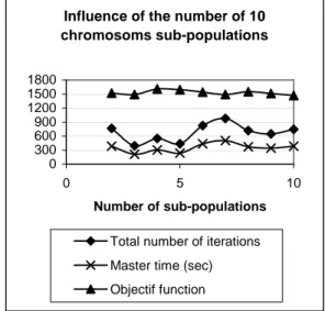
- the number of sub-populations: this parameter was fixed to 5 because is seem to be the best compromise between solution time and computing resources (figure 5).
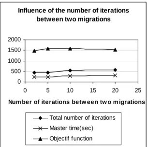
- The number of iterations between two migrations is chosen, as in the literature, equal to 5 (figure 6).
As can be seen on figure 7 for the ammonia synthesis loop, the distributed genetic algorithm requires less time than the global parallelisation. Moreover, it appears that the values of the objective function are better in the case of distributed genetic algorithms.
5. CONCLUSIONS
The proposed method allows to design redundant sensor networks for chemical plants. The optimised networks are much cheaper than the one containing all possible sensors. Moreover, accuracies on key parameters are acceptable.
Parallelisation methods allowed to reduce the computing time in an acceptable way for small and medium problems. However, the design of sensor
networks for larger plants like refineries can still not be considered nowadays but suboptimal solutions can be obtained by treating individual plant sections. The two parallelisation methods that were tested allowed to reduce the solution time but distributed genetic algorithms appeared to be better than global parallelisation.
6. REFERENCES
Bagajewicz M.J., 1997, « Process Plant Instrumentation: Design and Upgrade », chapter 6, Technomic Publishing Company
Goldberg D.E., 1989, « Genetic Algorithms in Search, Optimization and Machine Learning », Addison-Wesley
Gropp W., Lust E., Skjellum A., 1999, « Using MPI: Portable Parallel Programming with the Message Passing Interface », Second Edition, The MIT Press
Herrera F., Lozano M., Moraga C., November 1999, « Hierarchical Distributed Genetic Algorithms », International Journal of Intelligent Systems, Volume 14 (11), 1099-1121
Heyen G., Maréchal E., Kalitventzeff B., 1996, « Sensitivity Calculations and Variance Analysis in Plant measurement Validation », Computers and Chemical Engineering, volume 20S, 539-544 Madron F., 1992, « Process Plant Performance
Measurement and Data Processing for Optimisation and Retrofits », section 6.3, Ellis Horwood
Influence of the number of iterations between two migrations
0 500 1000 1500 2000 0 5 10 15 20 25
Number of iterations between two migrations
Total number of iterations Master time(sec) Objectif function
Figure 6: distributed genetic algorithm: influence of the number of generations between two migrations in the case of an ammonia synthesis loop
Time comparison between global parallelisation and distributed
algorithm 0 100 200 300 400 500 600 700 800 0 2 4 6 8 10
Number of processors or sub-populations
T im e ( s e c )
Global parallelisation : master time Global parallelisation : elpased time Distributed algorithm : master time Distributed algorithm : elapsed time
Figure 7: time comparison between global parallelisation and distributed genetic algorithm
Influence of the number of iterations between two migrations
0 500 1000 1500 2000 0 5 10 15 20 25
Num ber of iterations betw een tw o m igrations
Total number of iterations Master time(sec) Objectif function
Figure 6: distributed genetic algorithm: influence of the number of iterations between two migrations
![[PDF] Elaboration d’algorithmes itératifs en PDF | Cours informatique](data:image/gif;base64,R0lGODlhAQABAIAAAP///wAAACH5BAEAAAAALAAAAAABAAEAAAICRAEAOw==)