AGROCAMPUS OUEST CFR Rennes
Academic year: 2018 – 2019 Specialty : Agroecology
Mémoire de Fin d’Etudes d’Ingénieur de l’Institution Supérieur des Sciences agronomiques, agroalimentaires, horticoles et du paysage
Can traits help us understanding the response of weed
flora to viticultural practices?
By: Cécile Blanchet
Defended in Rennes on the 11th of September In front of the examinations board composed by:
President: Guenola Pérès
Supervisors: Guillaume Fried and Stéphane Cordeau
Referent teacher: Manuel Plantegenest
Jury member: Audrey Alignier
Les analyses et les conclusions de ce travail d'étudiant n'engagent que la responsabilité de son auteur et non celle d’AGROCAMPUS OUEST Ce document est soumis aux conditions d’utilisation
Table des matières
Acknowledgments ... Glossary ... Abbreviations ... Figures and tables’ lists ...
Introduction ... 1
Material and methods ... 6
I. Data acquisition ... 6
I.1. Vegetation survey ... 6
I.2. Environmental variables... 7
I.3. Agricultural practices ... 8
I.4. Plant traits ... 8
II. Data analyses ... 9
II.1.1 Weed community diversity ... 9
II.1.2 Weed community functional structure and composition ... 10
II.2. Characterization of management practices through environmental conditions ... 10
II.3 Statistical analysis ... 11
Results ... 13
I. Analysis of weed functional strategies (Grime’s strategies) ... 13
I.1. Axes of specialization of vineyards weeds ... 13
I.2. Vineyards weed functional traits related to Grime’s strategies ... 13
I.3. Describing the fidelity index to the inter-row by the traits’ variables ... 14
II. Influence of environment on weed community (functional) diversity ... 14
II.1. Effect of conventional and organic production mode ... 14
II.2. Effect of management practices ... 14
II.3. Relationship between the traits and the environmental variables ... 15
III. Influence of environmental variables on weed community functional composition ... 16
III.1. Effects of conventional and organic production mode ... 16
III.2. Effects of management practices ... 16
III.3. Relationships between traits and environmental variables (climate, soil properties, landscape) and management practices ... 17
Discussion ... 19
Conclusion ... 25 References ... Appendices ...
Acknowledgments
I would like to express my deepest appreciation to all those who provided me the possibility to complete my internship and my report.
A special gratitude I give to my supervisor, Guillaume Fried, who was always present, kind, patient with me, good mentor given amazing advice on functional approach, botany, statistics and writing report.
I would like to acknowledge my second supervisor, Stéphane Cordeau, for his advices, his time and his advice on my analyses and my report.
I also would like to thank the ANSES team, who was always nice to me, helping me when I asked for it and advising me.
I am grateful to Lorelei Cazenave for her complete database on Bordeaux vineyards and for having answer my questions.
I would like to acknowledge Aurélie Metay, Elena Kazakou, Jean and Virginie Thiebaut for the field trips on vineyard measuring plant traits, identifying some plants and for the good atmosphere.
I would like to thank my teachers for validate this internship and for the master 2 year in Agroecology.
A special grateful I give to Tiana Rakotoson, my office mate, for sharing the same office during six months, for listening me, helping me on many subjects (work (R!) or other), for the numerous breaks and for being a real friend.
I also want to thank all the interns in CBGP and Cirad, Camille Mayeux and Pauline Schnell for accepting me since the first date, your support, your joy and your friendship, Jérémie Fandos, Justine Chartrain, Pauline Farigoule and Héléne Joie for the breaks, the ping-pong games and the cakes time, and the Cirad team: Théo, Anthony, Hans, Matthias, Madiou, Julien, Yuan for the lunches and the never made volley game.
I would like to thank my family and my family in law for their support and kindness all along my internship but also my whole life. I know you always be here for me and me for you.
A special thanks to my Chouchou, Jérémie Gonella, for being always with me supporting me and encouraging me every day of my life, all of this wouldn’t be possible without you. I love you.
Glossary
Annuals: Plant with a life cycle under 1 year which grows once a year (Chauvel et al., 2018).
AMPA: AminoMethylPhosphonic Acid (one of the primary product degradation of herbicide glyphosate).
AUREA: Laboratory of analysis and advice agro-environmental.
Community: Species gathering which occupy the same area at the same moment (Chauvel et al., 2018). Competitor: capacity to absorb resources on fertile soil without disturbance or stress, big root system, important height and high SLA.
CWM: average trait value for a unit of biomass within a community (Kazakou et al., 2016)
ECOVITI: this network was created in 2010 by IFV (French institution of wine and vineyards). Its aim is to experiment an “organic winemaking possible economically and ecologically responsible in comparison with herbicides”. For that, it tries to settle a method with low inputs at national level providing communication and training to the winegrower (Cazenave, 2017).
Ecosystem: a dynamic complex of plant, animal and microorganism communities and their non-living environment interacting as a functional unit (Millennium Ecosystem, 2005).
Engrais verts (Green manure): plots lead by the chamber of Agriculture of Gironde for making test on green manure (Cazenave, 2017).
Epamprage: prick out the unfruited branches of the vines (IVF Occitanie).
Filters: Processes or constraints hindering the establishment or eliminating a species in a community (Fried and Maillet, 2018).
Functional richness (FRic): measured how the niche was occupied by the species and if it was optimally used or not (Schleuter et al., 2010).
Geophytes: Each year, decrease of the entire plant as underground part composed by the storage organ (a lot of plants with bulbs) (Navas and Garnier, 2013).
GIAF: network of plots followed since 2010 by the chamber of Agriculture of Gironde. The aim is to develop natural vegetation, try green manure practices and organic matter inputs (Cazenave, 2017). Gradient of disturbance: the varying factor leading to a partial or total destruction of plant biomass (White and Picklett, 1985; Grime, 2001).
Gradient of resources: the varying factor is the resource needed by the plant to grow and breed as light, water, C02, minerals, etc (Navas and Garnier, 2013).
Hemicryptophytes: Regular decrease of aerial system at its basal part, consequently the future buds will be near the soil surface during the bad season (a lot of Gramineae and plants with rosettes) (Navas and Garnier, 2013).
Perennials: species which breed, live long time as vegetative way (stolon, rhizome, bulb…) (Chauvel et al., 2018).
Ruderal: species have as characteristic to acquire available resources quickly, to grow very fast and to produce numerous small seeds (Fried et al., 2019).
Specification (“cahier des charges” in French): Strict rules in organic production mode to obtain a certification.
Stress-tolerant: grow in no productive areas with small height and low SLA.
SVBA/DEPHY network: network to exchange, communicate and try technical itinerary of farmers to decrease the chemical inputs. Created in 1995 and regrouped 140 winegrowers (Cazenave, 2017). Therophytes: plants of whom the aerial and underground systems die after seeds’ production and of whom close the cycle less than a year (a lot of annual plants in cultivated areas) (Navas and Garnier, 2013).
Trait: is any morphological physical or phenological feature measurable at the individual level from the cell to the whole-organism level, without reference to environment or any level of organization (Violle et al., 2007).
Abbreviations
Abun: Abundance
AIC: Akaike Information Criterion ANOVA: Analysis of variance CA: Correspondence Analysis
CA33: Chamber of Agriculture of Gironde (33)
CIVB: Conseil Interprofessionnel des Vins de Bordeaux CWM: Community Weighted Mean
CWV: Community Weighted Variance
EPPO: European Plant Protection Organization FD: Functional Divergence
FE: Functional Evenness FR: Functional Richness GLM: Global Linear Model
HCA: Hierarchical Cluster Analysis IR: Inter-Rows
IQR: InterQuartile Range
IVF: French Institute of wine and Vineyards PCA: Principal Component Analysis
PRA: small agricultural regions (Petites Regions Agricoles in French) R: rows
S: Species richness
SHDI: Shannon’s Diversity Index SLA: Specific Leaf Area
TCA: Total Cultivated Area (Surface Agricole Utile (SAU) in French) TFI: Treatment Frequency Index
Figures and tables’ lists
Figures
Figure 1: Location of the 101 plots of vineyards (Cazenave, 2017)
Figure 2: Scheme describing the method to provide the floristic sampling of each plot (took back from Varela (2015))
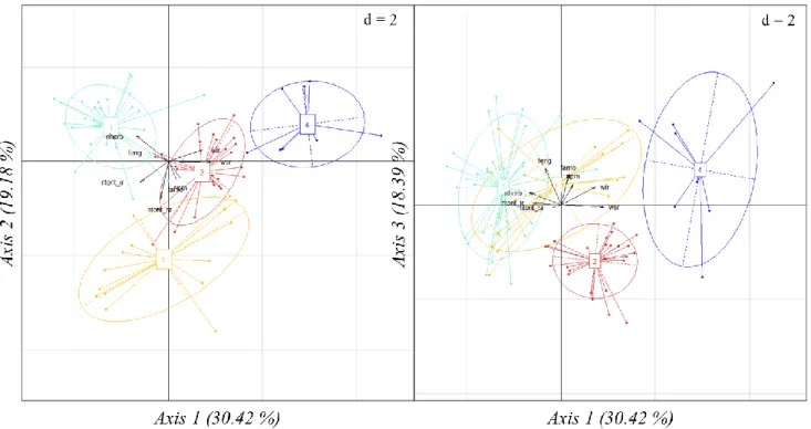
Figure 3: Hill & Smith analysis displayed with the quantitative variables in black marked out by an arrow, the qualitative variables in blue and the supplementary variable: The Fidelity Index in the inter-rows in red marked out by an arrow.
Figure 4: Grime strategies as supplementary variables on the Hill & Smith (a), C: Competitor, S: Stress-tolerant and R: Ruderal, and the significance of the distribution along the 1st axis (b) and the 2nd axis (c).
Figure 5: Diversity indices: i.e. the species richness (a,b), the abundance (c,d), the functional richness (e,f) and the Rao’s quadratic entropy (g,h), according to the area (inter-rows in blue, rows in red), the mode of production called here certification (conventional in orange and organic in green). The horizontal bar of the boxplot represents the median, 50% of the values were located from the 1st quartile
to the 3rd quartile (interquartile range, IQR). Blacks dots are values higher or lower than 1.5 the IQR.
Figure 6: Boxplots of the repartition of the four groups depending on the diversity’s indices: Species richness (a), Abundance (b), Functional richness (c) and Rao’s quadratic entropy (d). The inter-rows were represented in dark grey and the rows in pale grey, the group 1 is in yellow, the group 2 in red, the group 3 in green and the group 4 in blue.
Figure 7: Results of the global RLQ (101 fields) for the traits (on the left) and the species (on the right) Figure 8: Results of the global RLQ (101 fields) for the environment variables (on the left) and the field (on the right)
Figure 9: Fourth corner analysis of the global dataset (101 fields) on the left and adjusted fourth corner analyses of the three datasets (global, rows, inter-rows) on the right. The red cells represented the positive associations and the blue cells represented the negative associations. The non-significant cells were represented in grey. The upper left triangles represent the inter-rows significant interaction, the bottom right triangles the rows and the empty squares the global interaction.
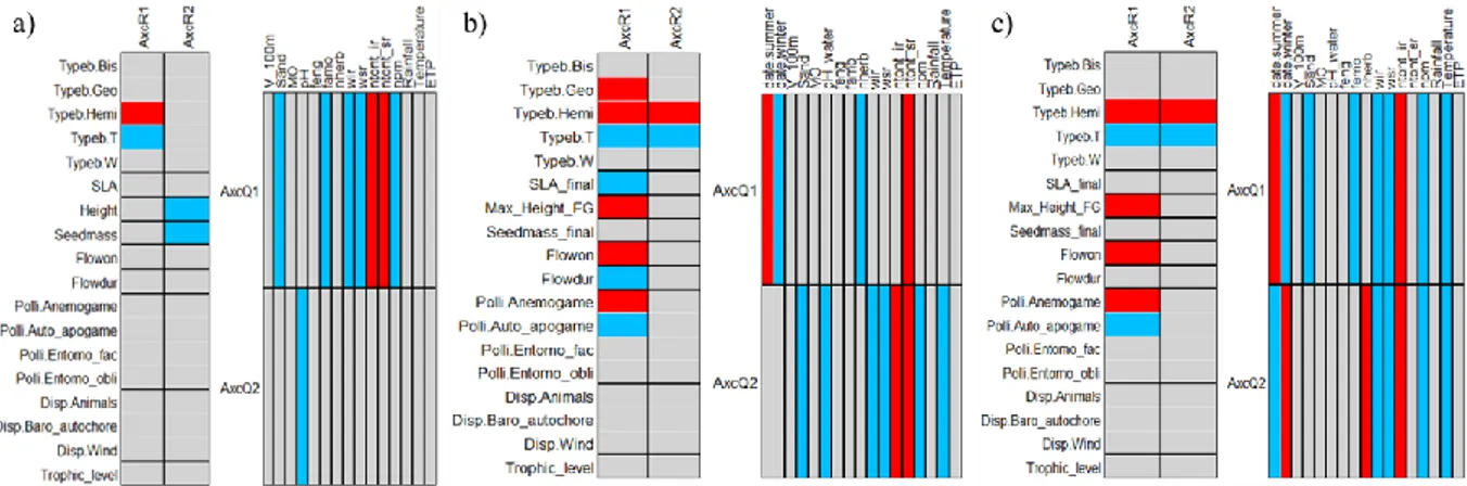
Figure 10: Results of the combination of the RLQ and the fourth-corner analyses for the global (a), the rows (b) and the inter-rows (c) analyses. On the left of each table, the fourth-corner tests between the two axes of the RLQ for the environmental gradients and the practices (AxcR1/AxcR2) and traits. On the right of each table, fourth-corner tests between the two axes of RLQ for traits (AxcQ1/AxcQ2) and the environmental variables and the practices.
Tables
Table 1: Evaluation table of frequency inspired by Theau et al. (2010) Table 2: Evaluation table of abundance according to Braun-Blanquet (1934) Table 3: Description of climate variables
Table 4: Description of the soil properties
Table 5: Description of the selected landscape variable Table 6: Description of the agricultural practices Table 7: Description of qualitative traits
Table 9: Species with high fidelity index to the inter-rows (green on the left), fidelity index close to zero (orange in the middle) and high fidelity index to the rows (red on the right)
Table 10: The F_value, the estimate and the significance concerning the habitat, the production mode and the interaction between both, for the species richness, the abundance, the functional richness (FRic) and the Rao’s quadratic richness. The points (.) indicated a p_value above 0.05, the stars indicated a p_value between 0.05 and 0.01 with a star (*), a p_value between 0.01 and 0.001 with two stars (**) and a p_value under 0.001 with three stars (***). The adjusted R² indicated the contribution of the model to the diversity’s indicators.
Table 11: F_value of linear models with interaction of the diversity’s indices. The point (.) indicated a p_value above 0.05, the stars indicated a p_value between 0.05 and 0.01 with one star (*), a p_value between 0.01 and 0.001 with two stars (**) and a p_value under 0.001 with three stars (***).
Table 12: Linear models given the F_value and the estimate for the four indices of diversity: species richness (S), abundance (Abun), functional richness (FRic) and the Rao’s quadratic entropy (Rao). A compartment in color is significant, green for the positive interactions and yellow for the negative ones. The point (.) indicated a p_value above 0.05, the stars indicated a p_value between 0.05 and 0.01 with one star (*), a p_value between 0.01 and 0.001 with two stars (**) and a p_value under 0.001 with three stars (***).
Appendices
Appendix I: Histograms of diversity’s indices, CWM and CWV of traits
Appendix II: Inertia’ tables explaining the traits’ distribution to the axes of the Hill & Smith analysis applied on the matrix Q
Appendix III: Groups results after performing a PCA and a HCA on the practices (101 plots)
Appendix IV: PCA performing to choose environmental variables including the climatic conditions, landscape, the soil properties and the management practices for linear models
Appendix V: Production modes’ influence (organic/conventional) on CWM and CWV of traits Appendix VI: Influence of groups of practices on the CWM and CWV of traits
Appendix VII: RLQ analyses of the rows (a) and the inter-rows (b) Appendix VIII: Linear model for CWM and CWV of traits
Introduction
History of viticultural practices
The French vineyards represent a part of the French heritage since the Antiquity (Dion, 1977). Until the beginning of the twenty-one century, the French production and quality were considered as the best of the world even if all French wines do not present high quality (Phillips, 2016). Despite the improvement of wine quality in new countries such as USA, Chile, South Africa or Australia, France still has a top position in the wine world and on the market. In 2018, France is the second wine maker in Europe and in the world with 46.4 million hectoliters of wine for 755 00 hectares of production (Alim’agri, 2018).
The vine (Vitis vinifera) is a perennial plant grown as monoculture and need several operations during the season to manage the field, to obtain a reasonable yield and grape quality. The fungi management (mildew, powdery mildew) represents the main part of the pesticide treatments (around 16 treatments of 20.1 in Agreste, 2019). Although fewer in number, herbicide treatments (around two for herbicides and epamprage in Agreste, 2019) are pointed out in wine-growing regions because herbicides or their metabolites (e.g. AMPA) were the most commonly molecules found in water. Herbicides are used to avoid competition between weeds and vines for light and water, in order to save yield (Kazakou et al., 2016; Gaba et al., 2017) and to limit the availability of shelter for pests (Gaba et al., 2017).
The definition of weeds varies among the authors but a lot of them agree to say that a weed is an unwanted plant growing in a place managed and disturbed by humans (Baker, 1974; Randall, 1997; Radosevich at al., 2008). Eleven thousand years ago, the first farmers selected plants for their needs (the crops) keeping the others aside and considering them as weeds (Gasquez, 2018). Nowadays and in this study, we consider that weeds can be both a major problem for crop production (Radosevich et al., 2008; Kazakou et al., 2016) but also, they are tools able to provide ecosystems services as reducing soil erosion for example (Ruiz-Colmenero et al., 2013). For this study, the definition of weeds will follow the one of Fried (2019) that defines a weed as all non-cultivated plants which grow in a cultivated plot, whatever their status. Usually, several weed species grow together in the same cultivated plot and form weed communities whose composition and diversity are determined by abiotic and biotic filters. Filters are processes or constraints hindering the establishment or eliminating a species in a community (Fried and Maillet, 2018). The weeds can be associated to ecological strategies based on the competition (C), the stress (S) and disturbance (D) according to Grime (Grime, 1974). Grime’s CSR strategies are usually used to compare flora in cultivated areas and to describe weeds communities (Gaba et al., 2014, Kazakou et al., 2016; Fried et al., 2019).
To control the potential adverse effects of weeds, tillage was usually applied on the vineyards before the 1970’s to weed the rows and the inter-rows (Barralis et al, 1983; Maillet, 1992). From the 1970s the first authorized vine herbicides were put on the market.
Chemical weeding was gradually adopted, first located on the rows, maintaining superficial tillage on the inter-rows, then carried out “in full” (rows plus inter-rows) with complete abandonment of all soil tillage operations (Maillet, 1992). These changes of management practices lead to major evolutions on weed communities. Tillage or herbicides have selected certain types of weeds called ruderal according to the Grime’s theory (Grime, 1988). These ruderal species are prone to acquire available resources quickly (between two disturbances events), to grow very fast and to produce numerous small seeds (Fried et al., 2019). The combination of no-tillage and herbicides in vineyards allows the colonization of vines by perennial plants, even woody species, whose deeps roots are difficult to reach even with herbicides (Montégut, 1982).
The massive use of herbicides has also provoked a huge decline of species diversity as well as a decrease of the abundance per species (Barralis, 1983) and can have unintended effect on other species than the target ones (Fried and Maillet, 2018). Moreover, the herbicides are responsible for water pollution (Martı́nez et al., 2000; Louchart et al., 2001) and it becomes a priority to reduce them. Nowadays, this challenge is taken into account by the government with the decrease of the number of actives molecules retired from the market (from 21 in 2001 to 11 in 2012, Gaviglio, 2013). Moreover, more and more vineyards adopted an organic management (in 10 years, the number of organic vineyards has tripled and in 2016 it represents 9% of the total number) increasing the use of tillage in the inter-rows (Agence Bio/OC, 2017).
A new challenge: reducing inputs to take advantage of the ecosystem services
Many ecosystem services can be provided by the weed communities if they are well managed. First of all, the competition between the weeds and the wine grape decreases the strength of the vines improving the grape quality (increasing the alcohol content, diminution of acidity…) (Van Leeuwen and Seguin, 1994; Pellegrino et al., 2005) and decreases the vineyards works as epamprage, thinning out of leaves or clipping and improves the microclimate, which decreases the fungal diseases. Secondly, the weeds can provide trophic resources, shelters, wintering and reproduction areas for pollinators, granivore arthropods, herbivorous and omnivorous, birds and mammals (Bàrberi et al., 2010), better pest regulation by favoring the crop auxiliaries as earthworms or Carabidae (balance between pests and crop auxiliary), pollination services (sexed reproduction, biofuel production or medicines with vegetal origins) and grains (Kazakou et al., 2018). The earthworms and the dynamics of microorganisms present in the soil can increase the quality of the soil allowing the minerals’ retention (less nitrogen lixiviation and more carbon sequestration). A better soil increases the water service during the winter period and improves the water’s quality. For all these reasons, there is an important tendency in vineyards to leave a certain amount of vegetation in the vines. This vegetation includes weed species that are spontaneous (Boisson, 2016) and sometimes also a cover crop which consist of one or several chosen species deliberately sown by winegrowers (Metay et al. 2018).
These cover crop constitute a service crop (Garcia et al., 2018). They can be temporary sown, as barley (left in winter and terminated in spring), or permanent, such as tall fescue (Celette et al., 2010). They are mainly sown in the inter-rows (less in the rows to avoid competition) but with different pattern, i.e. sometimes every inter-row, one inter-row over two, one inter-row over three, etc (Metay et al., 2018). The management of the rows and of the inter-rows is often different because of the proximity of vines in the rows and the width of the inter-rows which allow the use of mechanical tools (Metay et al., 2018). Alternative physical tools exist to regulate the weeds such as mowing, mechanical and thermic weeding, mulch and more traditional practices such as the crushing of wine branches, the rolling or the grazing (Metay et al., 2018). However, studies about the effects of these alternative practices remain scarce and do not allow to advise winegrowers properly on how to manage weeds in both the spontaneous cover or cover crop situations.
Using a trait-based approach to explain and predict relationships between management practices and weed communities
Classical studies on the ecology of weed communities have tried to link management practices to a given species composition (Barralis et al, 1983; Gago et al, 2007). This taxonomic approach shows some limits which can be partially overtaken by the functional approach. This latter approach is inspired by the functions performed by the plants and the role of species in the ecosystems. The concept was born in the 19th century with Von Humbolt (1806) in Grime and Pierce (2012) but was only developed
during the 20th century and has been widely used by the ecologists for 20 years. As the functions of
species are hard to reach and measure, proxies, called traits, are used to obtain information on these functions. The term “traits” has been widely used with various meanings. Violle et al (2007) proposed a definition that is widely agreed upon: “a trait is any morphological physical or phenological feature measurable at the individual level from the cell to the whole-organism level, without reference to environment or any level of organization”. That means nothing around the species traits, environmental factors nor population is necessary to describe the traits (of course, when measuring the trait values, it remains important to characterize the environment). The main interest of using the traits is to generalize the links between the practices and the flora.
In comparison to cultivated fields with annual crops where the concept was largely applied (Fried et al., 2009; Gunton et al., 2011; Fried et al., 2012), the vineyard appear as an ideal model to improve our understanding of weed responses to various types of disturbances thanks to a higher diversity of management practices applied in vineyards over the last decades (Gago et al., 2007). The present study takes place in the Bordeaux Wine Region and is part of the VERTIGO project (supported by the CIVB) following the thesis of Lorelei Cazenave (2017). The aim here is to characterize the response traits of weeds to viticultural practices. Thus, questions occur in accordance to this aim:
▪ (1) What are the different weed strategies (combination of traits) beyond the diversity of weeds in vineyards?
▪ (2) To what extent can these strategies be related to the contrasted management practices in the rows and in the inter-rows and to the environmental gradient (soil, weather, landscape)? i.e. are rows and inter-rows harbouring different weed communities?
▪ (3) Do the management practices in vineyards (tillage, mowing, herbicides, fertilization) act as filters on plant traits? What are the main traits that respond to different gradients of management practices?
▪ (4) Finally, from a methodological point of view, we asked what is the best strategy for analyzing the influence of management practices on weeds between: i) the use of broad but integrative classification as organic versus conventional mode of production, ii) the use of ‘cropping systems’ identified as homogeneous groups of vineyards plots using similar practices, iii) the use of the raw management practices variables?
To answer these questions, the weed communities will be analyzed to understand their composition and their functioning thanks to the Grime’s strategies (Grime, 1988). Then, the impacts of management practices and other environmental variables will be studied through the three levels of analyses (see the question #4) on the weeds’ diversity and on the trait’s values.
Hypotheses
(1) It exits different ecological strategies which can be based on the reproduction, the adaptation, the resources or the functional traits. The Grime’s CSR strategies will be used to answer the question of weed strategies. The first hypothesis is that as in all cultivated area, the flora in vineyards is essentially composed by ruderal species because of the high level of disturbances. One the other hand, the vineyard can be managed with a diversity of practices. For example, herbicides can be applied only in the rows and mowing only in the inter-rows (Metay et al., 2018). Different management practices can also be applied on the same area (rows or inter-rows) at different period, such as mowing followed by tillage (MacLaren et al., 2019). Therefore, the second hypothesis is that with this diversity of practices through time and space the weeds communities will adopt different strategies.
(2) Studies showed that season and latitude (location of the plots) can be the main filters to weeds communities (Fried et al., 2019), whereas others studies showed that the main impact on weed communities are management practices (Lososovà et al., 2002; Kazakou et al., 2016). The first hypothesis is that the abiotic filters as weather, soil properties and landscape will shape the weed communities and as they are similar on the same plot, the rows and the inter-rows weed communities will be identical whatever the practices.
The second hypothesis is that different management practices in the rows and in the inter-rows will translate on the fields by different communities in the both areas for diversity and traits.
(3) The practices applied on vineyards act as filters on plant traits (Lososovà et al., 2003; Kazakou et al., 2016; Gaba et al., 2017; MacLaren et al., 2019). Even Fried et al. (2019) showed a tiny impact of management practices after the season and the latitude influence on weed communities.
The first hypothesis concerns the influence of management practices on weed communities’ diversity. The hypothesis 1.A. is that the practices will impact the taxonomic and the functional diversity by direct (herbicides) and indirect effects (soil compaction through the number of mechanical passages) (Hole et al., 2005; Bruggisser et al., 2010). The hypothesis 1.B. is that the practices are not responsible for the difference of diversity between production mode (Nascimbene et al., 2012).
The second hypothesis concerns the combination of traits found under different gradients of disturbance. The hypothesis 2.A. is that a high gradient of disturbance will favor traits values associated to ruderal strategy with high SLA, small height and low seed mass (Grime, 1988), with early flowering onset (Garnier et al., 2016), as under mechanical passages. At the opposite, the trait values in low disturbed areas will follow competitive strategy (gradient of resources) with high maximum height, high SLA and small seeds (Kazakou et al., 2016). High disturbance can be associated to the use of pesticides which can be associated to a low level of pollinators. So, the self-pollination and dispersal can be expected in this context (Fried, 2019). Besides, the higher is the disturbance, the more we expect a convergence of the traits (especially for tillage) whereas the lower is the disturbance, as for mowing, the more we expect a divergence of traits (Kazakou et al., 2016).The hypothesis 2.B. is that weeds will have other traits as the traits of ruderal strategy to overpass the management practices (Garnier et al., 2016). The traits will be a low SLA (to invest in the plant structure, less permeability to herbicides) and a high seed mass under tillage management to be able to emerge from deeper in soil and to be able to grow (Armengot et al., 2016). The maximum height will increase to acquire light faster under disturbed areas (MacLaren et al., 2019).
(4) Three approaches concerning the description of management practices will be applied. The first hypothesis is that the three approaches will be complementary and at each level the information will be more accurate. The second hypothesis is that the organic/conventional approach will not be enough accurate (MacLaren et al. (2019) used three levels of production mode), the raw variables at the opposite will give many information but hard to interpret, whereas the groups will be a good trade-off between the two other approaches.
Figure 1: Location of the 101 plots of vineyards (Cazenave, 2017)
Figure 2: Scheme describing the method to provide the floristic sampling of each plot (took back from Varela (2015))
Material and methods
I.
Data acquisition
I.1. Vegetation survey
All the floristic surveys were done in 2015 in the Bordeaux vineyards (Cazenave, 2017). This wine production region gets an oceanic climate and has vineyards growing on the sand, graves and silt-calcareous soil (Vin & vigne, 2015). Nowadays in Aquitaine, 50 % of the total cultivated area (TCA) produces wine grapes (Agreste, 2015). With the ECOPHYTO plan, which aims to reduce by 50 % the herbicides use until 2025 (Plan ECOPHYTO II, 2015), and the cover crop success in the Bordeaux, the chemical weeding is limited under the rows only (Agreste, 2019). Moreover, the treatment frequency index (TFI) of herbicides reaches 0.7 as the national mean (Agreste, 2019). One hundred and one101 plots belonging to 51 vineyards distributed in the Gironde (98 plots), the Dordogne (2 plots) and the Lot-et-Garonne (1 plot) departments were studied. The plots belong to five networks: GIAF (2x6 plots), ECOVITI (2x7 plots), Engrais Verts (2x12 plots), DEPHY/SVBA (52 plots) (defined in the glossary). One of the plots has been tilled before the floristic sampling (101 plots instead of 102). Figure 1 showed the distribution of the vineyards and their belonging to networks and to the small agricultural regions (Petites Regions Agricoles (PRA) in French).
A vineyard plot can be divided into three types of area: the rows, the tilled inter-rows and the covered inter-rows (spontaneous or sowed vegetation (i.e. cover crop)). The floristic sampling protocol developed by the Chamber of Agriculture of Gironde (CA33) (Varela, 2015) considers this heterogeneity. For each area (rows, tilled and covered inter-rows), the sampling method was to record all species over 50 m length (2 x 25 m, around 10 vineyard stakes) with a width of 1 m, that corresponded to a total of 150 m²/plot (Figure 2). The rows (R) and the inter-rows (IR) were randomly chosen as the beginning zone for the sampling. The only rule was to avoid the edge effect, so it had to begin after 2 stakes from the edge. For the plots where the inter-rows were only tilled, the sampling was performed on two inter-rows to obtain the same surface per plot.
For each species, the frequency and the abundance were noted. Frequency was based on the presence/absence of the species on 10 sections of 5 m with a resulting frequency ranging between 1 (one individual) and 5 (species present in all the sections) (Cazenave, 2017) (Table 1). Abundance was obtained thanks to the cover percentage of each species per plot. The method comes from Braun Blanquet et al. (1934) which describes the abundance with 5 categories going from 1 for the isolated species (cover <5%) to 5 for species forming a continuous carpet (cover > 75%) (Table 2). To end, frequency and abundance were multiplied to obtain the percentage of cover of each species per plot. The species were identified in the database with their scientific, common and EPPO names (http://eppt.eppo.org/).
Table 1: Evaluation table of frequency inspired by Theau et al. (2010)
Table 2: Evaluation table of abundance according to Braun-Blanquet (1934)
Class Covering Mean density (D2)
1 Species covering 1% to 5% 0.025
2 Species covering 5% to 25% 0.15
3 Species covering 25% to 50% 0.375
4 Species covering 50% to 75% 0.625
5 Species covering 75% to 100% 0.875
Table 3: Description of climate variables
Climatic variables Definition Mean – sd Min – Max
Rainfall (mm/year)
Average on the year 2015
674.50 ± 46.32 593.68 – 848.52
Temperature average (°C/year) 12.45 ± 1.23 10.32 – 14.10
Evapotranspiration (mm/day) 2.67 ± 0.08 2.47 – 2.89
Table 4: Description of the soil properties
Abbreviations Definition Unit Mean – sd Min – Max
Pl_A Clay percentage % 19.04 ± 10.79 2.7 – 54.9
Pl_L Silt percentage % 33.35 ± 17.37 5.1 – 70.7
Pl_S Sand percentage % 47.81 ± 23.51 3.0 – 87.2
Pl_CaCO3 Calcareous content in the soil g/kg of soil 34.15 ± 71.60 0.0 – 271.0 Pl_MO Organic matter content in the soil g/kg of soil 1.82 ± 0.81 0.4 – 4.58
PD_CN Carbon/Nitrogen ratio No unit 10.28 ± 2.57 4.0 – 17.4
PD_PH_EAU pH measured with water No unit 7.49 ± 0.99 5.3 – 12.7
PD_PH_KCl pH measured with KCl No unit 6.33 ± 0.91 4.1 – 7.9
PD_CEC Cation exchange capacity mol/kg of soil 9.13 ± 4.85 2.8 – 24.8
PD_P2O5 P2O5 content g/kg 0.095 ± 0.090 0.01 – 0.451 PD_K20 K20 content g/kg 4.01 ± 37.76 0.043 – 374
PD_MgO MgO content g/kg 0.24 ± 0.16 0.042 – 0.82
Table 5: Description of the selected landscape variables
Abbreviations Definition Unit Mean – Sd Min – Max
Surf Surface of the plot Square meter (m²) 7776 ± 4905 784.1 – 24580
Slope Angle of the slope degree (°) 2.61 ± 1.75 0.307 – 9.07
V_20 m Vineyards 20 m radius % 50.97 ± 17.06 5.45 – 84.33
V_100 m Vineyards 100 m radius % 77.26 ± 17.32 29.42 – 100
Class Frequency
1 Single individual
2 Rare species
3 Observed species every 4-6 stakes 4 Observed species every 2-3 stakes 5 Observed species every stake
The floristic sampling was made twice: the first one at the end of Marsh/ beginning of April before the first treatment (herbicides, tillage, mowing) were applied in the plot; and the second one at the end of June/beginning of July after that all management practices have been applied (tillage, herbicides treatment, mowing). In total, 541 floristic samples were made in 2015, containing 200 species of weeds. Because of the yearly alternation between tilled and covered inter-rows, the distinction between those two kinds of inter-rows was not relevant and when a plot contained tilled and covered inter-rows, the maximum of the density (D2) was taken. At the end, 400 floristic samples were describing the rows, the inter-rows and the sampling period (winter and summer). The table containing the maximum of density (D2) for each plot was named the matrix L.
I.2. Environmental variables
I.2.1 ClimateA partnership with the French Institute of Wine and Vineyards (IVF) allowed obtaining the climatic data for each plot, thanks to the TRYDEA tool. It gave the mean temperature, the mean rainfall and the mean potential evapotranspiration (Table 3) for each plot every day of the year 2015.
I.2.2 Soil properties
Soil was sampled at two depths: 0-30 cm and 30-60 cm, using an auger. On each plot: 6 auger samples were taken on 2 inter-rows of the vineyards and 6 others on 2 rows of the vineyards. The choice of the inter-rows and the rows were made randomly avoiding the edges of the plot. The analyses were performed by the AUREA laboratory based in Blanquefort (Gironde) (Table 4).
I.2.3 Landscape and topography
Landscape data can help understanding how the land cover around the studied plots influences weed community composition or diversity in the vineyards. The landscape database has been obtained in a previous study (Boisson, 2016) thanks to the ArcGis® software 10.1 and its extension ‘spatial analyst’, produced by the ESRI firm. To characterize the landscape, the proportion of each habitat types (urban zones, annual crops, perennial crops, water areas, grasslands, vineyards, forests and woodlands, as well as a miscellaneous category) was determined. Shannon’s Diversity Index (SHDI) was then calculated based on the number and relative proportion of the different habitat types, to represent landscape heterogeneity. Land cover and SHDI were computed for several buffer sizes: 50 m, 100 m, 250 m and 500 m radius around the plot. After running GLMs to explain weed species richness according to landscape diversity with different radius sizes, Boisson (2016) suggested to use the landscape metrics based on the 100 m radius according to the best model selected by the Akaike Information Criterion (AIC). The 100 m buffer size was considered as a good spatial scale to capture the percentage of vineyards and landscape diversity around the vineyard plots (Boisson, 2016). Moreover, the 20 m radius landscape was also kept because it represented the nature of the habitat at the edge of the plot, i.e. the most likely habitat to send plant propagules in the vineyard.
Table 6: Description of the agricultural practices
Table 7: Description of qualitative traits
Abbreviations Definition Unit Mean – Sd Min - Max
feng Chemical fertilization Number of fertilizations over the last 5 years (scale from 0 to 5)
2.13 ± 0.16 0 – 5
famo
Organic soil improver, return organic matter from the vine shoot and green manure.
Number of fertilizations over the 5 last years (Famo = Fam + Rmo, Fam: scale from 0 to 5 for the organic soil improver and Rmo: scale 0 to 10 for the vine shoot and green manure restitution)
6.46 ± 2.41 0 – 13
nherb
Herbicides which can be selective or not. They were applied on the rows only but can also have an impact on the inter-rows.
Number of herbicides passage per year
0.88 ± 1.05 0 - 3
wir Tillage in the inter-rows Number of passages per year x the number of inter-rows of the plot/2
1.77 ± 1.75 0 - 8
wsr Tillage in the rows Number of passages per year 2.21 ± 2.36 0 – 8
ntont_ir Mowing in the inter-rows Number of mowing per year x the number of inter-rows/2
3.50 ± 1.89 0 – 7
ntont_sr Mowing in the rows Number of mowing per year 0.62 ± 1.40 0 - 5
npm Number of mechanical passages Number of passages per year 26.7 ± 5.42 15 – 40
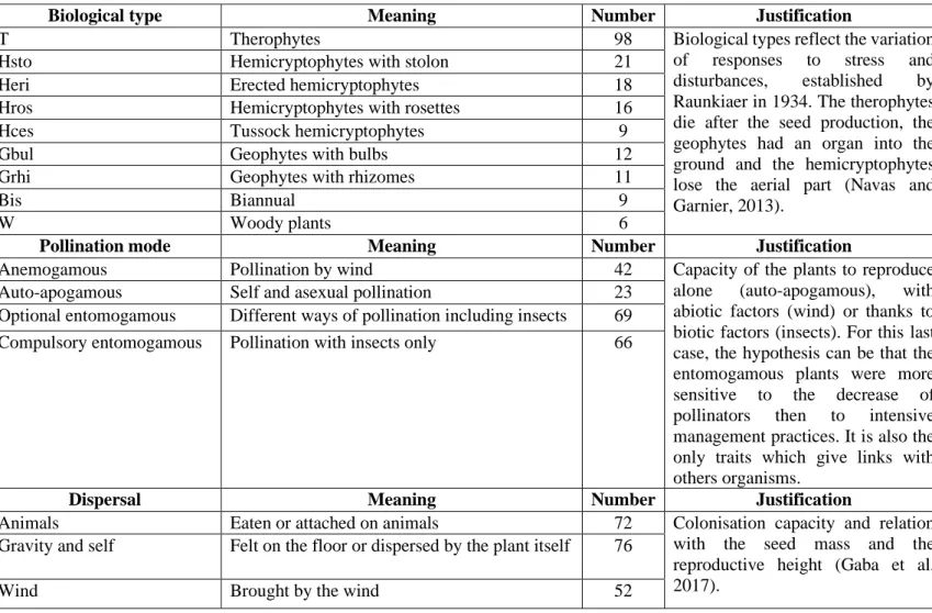
Biological type Meaning Number Justification
T Therophytes 98 Biological types reflect the variation
of responses to stress and disturbances, established by Raunkiaer in 1934. The therophytes die after the seed production, the geophytes had an organ into the ground and the hemicryptophytes lose the aerial part (Navas and Garnier, 2013).
Hsto Hemicryptophytes with stolon 21
Heri Erected hemicryptophytes 18
Hros Hemicryptophytes with rosettes 16
Hces Tussock hemicryptophytes 9
Gbul Geophytes with bulbs 12
Grhi Geophytes with rhizomes 11
Bis Biannual 9
W Woody plants 6
Pollination mode Meaning Number Justification
Anemogamous Pollination by wind 42 Capacity of the plants to reproduce
alone (auto-apogamous), with abiotic factors (wind) or thanks to biotic factors (insects). For this last case, the hypothesis can be that the entomogamous plants were more sensitive to the decrease of pollinators then to intensive management practices. It is also the only traits which give links with others organisms.
Auto-apogamous Self and asexual pollination 23
Optional entomogamous Different ways of pollination including insects 69 Compulsory entomogamous Pollination with insects only 66
Dispersal Meaning Number Justification
Animals Eaten or attached on animals 72 Colonisation capacity and relation
with the seed mass and the reproductive height (Gaba et al, 2017).
Gravity and self Felt on the floor or dispersed by the plant itself 76
Angaud (2018) performed a PCA on the landscape variables composed by SHDI and the different habitat types at 20 m and 100 m radii. She showed that the vineyard 100 m radius contributed the most to the construction of the axes and was positively correlated with the vineyard 20 m radius and the surface of the vineyard plot (m²) and was negatively correlated to SHDI. Therefore, we decided to summarize landscape variables by the percentage of vineyard that informed if the landscape around the studied plot was homogeneous or not, so if there was a source of diversity around.
The surface of the vineyard plot was also recorded. Previous studies have shown that there is a negative correlation between the size of the agricultural plots and the level of biodiversity (Fried et al., 2018). This correlation can be related to increase management intensity with higher field size or to a landscape configurational effect due to less field margin vegetation in landscape with large field size.
We also considered a topographic variable with the slope. The slope can have an influence on the species composition (Perring (1959) in Bennie et al., 2006) and can influence the magnitude of vegetation change (Bennie et al., 2006). Moreover, the slope influences also the practices: for example, the mechanical engines were difficult to handle in steep vineyard plots, so there are fewer tillage in this kind of plots while chemical control or spontaneous or cover crop are more often used to avoid the soil erosion (Vrsic et al., 2011). The surface, the slope, the proportion of vineyard in the 20 m and the 100 m radii were described in Table 5.
I.3. Agricultural practices
The management practices applied in the vineyard plots were gathered thanks to an electronic interview (google forms) of the concerned winegrowers. Based on a literature review (Gago, 2007), the main practices to consider for their effect on weed flora were: soil tillage (with the difference between rows and inter-rows), mowing (with differentiation between the rows and the inter-rows), and herbicides treatments, fertilizations (chemical or organic) and the total number of mechanized treatments (including diseases treatments, harvest…) (Table 6). This latter variable is the sum of the number of tractors passes which could be an indirect measure of soil compaction. The table containing all the environmental variables as climate, soil properties, landscape and agricultural practices was named the matrix R.
I.4. Plant traits
Different traits and ecological performance indicators were used in this study. These two types of indicators came from the data base BIOFLOR (Klotz et al., 2002) and baseflor (Julve, 1998). There were qualitative traits (Table 7) including the biological types, the pollination and the dispersal modes. There also were quantitative traits (Table 8) including the functional traits and the Ellenberg’s indicators, which characterize the response of species to environmental factors (Ellenberg et al., 1992). Ellenberg (1992) has listed these 6 indicators which were adapted to the central Europe conditions and Julve (1998) adapted it for the French vegetation. The matrix containing the traits was named the matrix Q (traits in columns and species in rows).
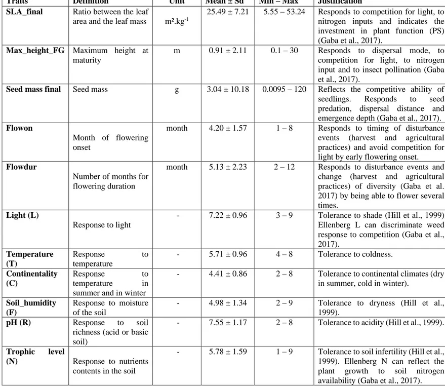
Table 8: Description of quantitative traits and ecological performance indicators (Units given by Bourgeois et al., 2019)
Traits Definition Unit Mean ± Sd Min – Max Justification
SLA_final Ratio between the leaf
area and the leaf mass m².kg-1
25.49 ± 7.21 5.55 – 53.24 Responds to competition for light, to nitrogen inputs and indicates the investment in plant function (PS) (Gaba et al., 2017).
Max_height_FG Maximum height at maturity
m 0.91 ± 2.11 0.1 – 30 Responds to dispersal mode, to competition for light, to nitrogen input and to insect pollination (Gaba et al., 2017).
Seed mass final Seed mass g 3.04 ± 10.18 0.0095 – 120 Reflects the competitive ability of seedlings. Responds to seed predation, dispersal distance and emergence depth (Gaba et al., 2017). Flowon
Month of flowering onset
month 4.20 ± 1.57 1 – 8 Responds to timing of disturbance events (harvest and agricultural practices) and avoid competition for light by early flowering onset.
Flowdur
Number of months for flowering duration
month 5.13 ± 2.23 2 – 12 Responds to disturbance events and change (harvest and agricultural practices) of diversity (Gaba et al. 2017) by being able to flower several times.
Light (L)
Response to light
- 7.22 ± 0.96 3 – 9 Tolerance to shade (Hill et al., 1999) Ellenberg L can discriminate weed response to competition (Gaba et al., 2017). Temperature (T) Response to temperature - 5.71 ± 0.96 4 – 8 Tolerance to coldness. Continentality (C) Response to temperature in summer and in winter
- 4.41 ± 0.86 2 – 8 Tolerance to continental climates (dry in summer, cold in winter).
Soil_humidity (F)
Response to moisture of the soil
- 4.98 ± 1.34 2 – 9 Tolerance to dryness (Hill et al., 1999).
pH (R) Response to soil
richness (acid or basic soil)
- 7.55 ± 1.17 2 – 8 Tolerance to acidity (Hill et al., 1999).
Trophic level
(N) Response to nutrients contents in the soil
- 5.78 ± 1.59 1 – 9 Tolerance to soil infertility (Hill et al., 1999). Ellenberg N can reflect the plant growth to soil nitrogen availability (Gaba et al., 2017).
In this study, the analyses are performed on a complete dataset. As the missing data represented less than 5% of the total dataset (2.6% (73/2800) for the matrix Q and 0.5% (16/3232) for the matric R), they were filled with predictive mean matching using the mice package. In order to avoid outliers, the seed mass and the plant height were log-transformed.
All the data were coming from the thesis or Lorelei Cazenave and some precisions were added thanks to Tristan Boisson for the landscape metrics and Maude Angaud for the number of variables. The addition and treatment of the plant trait data and the choice of the relevant variables for each analysis were the topic of this internship.
II.
Data analyses
II.1. Characterization of weed communities
II.1.1 Weed community diversityEach plot was first characterized by species richness (S), given the number of different species in a plot and the total abundance, the sum of abundance of all species in the plot. Then a number of indices were computed in order to describe the functional diversity and structure of the communities. Many studies showed that the species diversity was not enough to describe the ecosystem and that the functional diversity was needed to better understand their functioning (Tilman et al., 1997, Hulot et al., 2000, Díaz and Cabido, 2001, Heemsbergen et al., 2004 in Schleuter et al., 2010). The functional diversity can be defined by 3 types of indicators which are functional richness (FR), functional evenness (FE) and functional divergence (FD) (Schleuter et al., 2010), which are considered as independent in a random community. The first indicator taken is the functional richness (Fric), which measured how the niche was occupied by the species and if it was optimally used or not (Schleuter et al., 2010). The index used for this functional richness was coming from the hull volume of Cornwell et al. (2006) (Mason et al., 2013). The second indicator is the functional divergence represented by the Rao’s quadratic entropy. Rao's quadratic entropy gave the distance of traits between a pair of species and was a very used index for its flexibility (Schleuter et al., 2010). It represented a generalization of the Simpson index and can be calculated with the following formula (Leps et al. 2006):
𝐹𝐷(𝑅𝑎𝑜) = ∑ ∑ 𝑑𝑖𝑗. 𝑝𝑖. 𝑝𝑗
𝑆
𝑗=1 𝑆
𝑖=1
with S, the total number of species in the community, pi and pj, respectively the proportion of the species
i and j, dij the dissimilarity between the species i and j. dii = 0 because there was no dissimilarity in the
same species. If dij = 1, the pair of species was totally different, and another formula was used
(Botta-Dukàt 2005):
𝐹𝐷(𝑅𝑎𝑜) = 1 − ∑ 𝑝𝑖²
𝑆
The species richness and the abundance give information on the number of plants in the niche and the quantity of each of them. The functional indicators which are the functional richness (FRic) and the Rao’s quadratic entropic (Rao) bring more information on the functional side of the study with the comparison with an optimum thanks to FRic and a distance between the traits thanks to the Rao’s index. The Gower’s distance calculated for these two indicators allowed to compute distances for qualitative variables as the biological type and non-continuous variables as the Ellenberg indicators (c.f. I.4 Plant traits) (Karadimou et al., 2016). So, the four indicators were supplementary and described from different angle the diversity of the plots. The dbFD function returns FRic and Rao indicators per plot (Laliberté and Legendre, 2010).
II.1.2 Weed community functional structure and composition
The community weighted mean (CWM) and the community weighted variance (CWV) were calculated for each trait. CWM could be computed thanks to the dbFD() function, which took into account the relative abundance of species per each plot. The CWM values “represent the average of traits values for a unit of biomass inside a community” (Kazakou et al., 2016). For the qualitative traits, it gave the percentage of presence of each trait in each plot. The CWV was calculated for each plot only for the quantitative traits by this formula (Hulshof et al., 2013; Bestovà et al., 2018):
𝐶𝑊𝑉 = ∑ 𝐴𝑖 × (𝑡𝑖 − 𝐶𝑊𝑀)²
𝑆
𝑖=1
where Ai was the abundance of species i, and ti is the trait value of species i.
II.2. Characterization of management practices through environmental conditions
We chose to describe management practices by using an increasing level of complexity:i) First of all, we used a very raw but consistent and integrative classification of plots based on the production mode followed by the winegrowers: organic versus conventional farming.
ii) The second strategy for analysing the data was to identify homogeneous groups of plots based on similar management practices. This is based on the idea that beyond organic and conventional production mode, there can be differences (e.g., one can assume that there are different types of organic farming and different levels of intensity within conventional winegrowers). First, the table with the 101 plots described by the eight management variables were subjected to a Principal Component Analysis (PCA) followed by a Hierarchical Cluster Analysis (HCA). Four groups were identified using the optimal number of clusters given by Mantel statistic, which compared the original distance matrix and the binary matrices computed from the dendrogram cut at various levels (Borcard et al., 2011). The management practices that best discriminates the four groups were identified thanks to the test value (v_test), which calculated the gap between the global mean and the mean of a modality and allowed the groups’ description (catdes (FactoMineR) Husson et al., 2016).
iii) In the last strategy, we tested directly the influence of all the 14 raw management practices variables including the soil, the landscape and the climate on weed species (functional) diversity and composition.
II.3 Statistical analysis
II.3.1 Analysis of weed functional strategies
A Hill & Smith analysis was performed on the matrix Q (200 species x 14 traits). A Hill & Smith analysis is equivalent to a Principal Component Analysis (PCA) adapted to matrixes mixing qualitative and quantitative variables (Hill and Smith, 1976). The Grime categories competitors, stress-tolerant and ruderal (Grime, 1974) were added as supplementary variables. They allowed to understand the repartition of the species categories depending on the traits and see if it corresponded to the strategies described by Grime. Then a Kruskal Wallis test was applied followed by a Dunn test to understand the distribution of Grime strategies along the first axes.
On the same matrix Q, the fidelity index to the inter-rows was calculated to determinate the species that are specific to each area (rows and inter-rows) and then linked to the traits. This index was calculated from the Chytrý et al. (2002) formula:
𝜑 = 𝑁. 𝑛p − 𝑛. 𝑁𝑝 √𝑛. 𝑁𝑝. (𝑁 − 𝑛). (𝑁 − 𝑁𝑝)
with N the number of samples used (400 floristic samples), Np, the number of samples in the inter-rows (201 floristic samples), n, the number of occurrences of the species in the whole dataset and np, the number of occurrences of the species in the inter-rows. This index ranged from -1 (species associated to the rows) and 1 (species associated to the inter-rows) (Fried et al., 2019).
II.3.2. Influence of environmental variables on weed community diversity and on weed community composition
i) Linear models with interaction applied to the three methods
The statistics were performed on the three methods level: the production mode (conventional versus organic), the groups practices and the raw variables and the aim was to compare the influence of each method and of the area (rows/inter-rows) on the diversity (taxonomic: S, Abundance; functional: FRic, Rao) and on the traits (CWM and CWV). To obtain such analyses, linear models with interaction were performed on the 400 floristic samples. An ANOVA (type III) was applied to emphasize the significance of the diversity’s indicators and the traits’ values (CWM and CWV). For the production mode, the model significance was tested thanks to the glht function from the multcomp package (Tukey test). For the groups, the model significance was evaluated thanks to the testInteraction function from the phia package. And for the raw variables, the model was selected thanks to the Akaike Information Criterion (AIC). The AIC is an estimator of an expected distance developed by Kullback and Leibler (1951) which represents the loss of information between the reality and the model.
The aim was to maximize resemblance to the reality with the less variables as possible. The model chosen will be the one with the smallest AIC (Posada and Buckley, 2004). Then, the Shapiro test was applied on all linear models to verify the normality of the residuals of the ANOVA. The test was passed if the null hypothesis is accepted (p_value above 0.05). However, the dataset contained 400 floristic samples and Shapiro did not always work, so the normality was also evaluated on traits’ histograms (Appendix III). The variation inflation factor (VIF) was also applied to evaluate the collinearity into the model, if VIF value exceeded 10, the variables were removed from the models. A predictability of the model (repartition of the fitted results along the first bisector) was operated to assure the veracity of the model. The CWM of all biological types except therophytes, the flowering duration, the auto-apogamous and the facultative entomogamous and all CWV were sqrt-transformed to follow a normal distribution.
ii) Complementary approach and relationship between the environmental variables and the traits: RLQ – fourth corner analyses
Dray et al. (2014) developed an approach combining two analyses to show significant relationship between the traits and the environmental variables. For that purpose, a RLQ analysis was performed on the three matrices, the floristic matrix L, the traits matrix Q and the environmental matrix R. It is similar to a multivariate analysis which identify the best viewing of the “cloud’s points”. The RLQ displayed axes that best discriminates species (based on their traits) and sites (based on their environmental characteristics) and maximizes the covariance between environmental variables and the traits. It was the first step to have an idea of the correlation between the traits and the practices. Before the RLQ analysis, preliminary statistics were applied on each matrix. First, a Correspondence Analysis (CA) was performed on the floristic matrix L after a square-root-transformation on the matrix. This analysis was used as a canonical factor for the following analyses. Secondly, a Hill & Smith was performed on the traits’ matrix Q, which was scaled with the columns scores of the CA of the matrix L. Thirdly, a PCA was performed on the environmental matrix R, which was scaled with the rows scores of CA of the matrix L.
One of the drawbacks of the RLQ analysis is that it does not allow to make a direct correlation between the environment variables and a single trait. So, a second analysis was performed which is called the fourth-corner analysis. It realized simultaneously statistical tests on bivariate associations (one trait and one environment variable at a time). 9 999 permutations were made to adjust the p-value and the threshold of the significance was set at α = 0.05. However, this analysis does not consider the combinations of practices on one hand and the combinations of the traits on the other hand. So, the two analyses (RLQ and fourth corner) were combined to avoid their inconvenient when they are used separately.
Figure 3: Hill & Smith analysis displayed with the quantitative variables in black marked out by an arrow, the qualitative variables in blue and the supplementary variable: Fidelity Index in the
inter-rows in red marked out by an arrow.
Figure 4: Grime strategies as supplementary variables on the Hill & Smith analysis (a), C: Competitor, S: Stress-tolerant and R: Ruderal, and the significance of the distribution along the 1st
This combination of analyses allowed highlighting the significant correlation between the combinations of environmental practices and each trait, and the significant correlation between the combinations of traits and each management practice.
This approach was also implemented separately on the rows and on the inter-rows, and on the winter and the summer sampling periods, using the 400 floristic samples to test the influence of the areas (rows/inter-rows) and the sampling period (summer/winter), which were not considered in the global analysis performed on the 101 plots gathering the two sampling periods.
All the statistics ran thanks to the ade4, car, FactoMineR, FD, MASS, multcomp, phia and vegan packages and ggplot2 package displayed the figures.
Results
I.
Analysis of weed functional strategies (Grime’s strategies)
I.1. Axes of specialization of vineyards weeds
The aim of this Hill & Smith analysis was to highlight suites of traits associated to the fidelity of weeds to the IR and to interpret them in the light of the Grime strategies. We kept the first four axes of the Hill & Smith analysis which explained 35.86 % of the traits’ distribution (Figure 3, see the inertia table in Appendix II and contribution of the variable to the axes). The first axis was positively correlated with Ellenberg’s indicators for continentality (39.7 % of relative contribution to the construction of the axis 1) and for trophic level (34.6 %), flowering duration (39.2 %) and SLA (26.6 %). The first axis was negatively correlated with Ellenberg’s indicators for temperature (-37.1 %) and for light (-21.8 %). The second axis was positively correlated with therophytes (32.2 %) and negatively with maximum of plant height (-40.4 %) and flowering onset (-40.3 %). This second axis also opposed annual species (therophytes) to perennial species (various types of geophytes and hemicryptophytes).
I.2. Vineyards weed functional traits related to Grime’s strategies
The Grime strategies describe three types of species, the ruderals, the stress-tolerant and the competitors, and the combinations between the three types of species. The Figure 4.a) showed the belonging of each species to a Grime’s strategy according to species position in the trait multivariate space (Figure 3). It occurred a similarity between this graph and the Grime’s triangular model (1974) explaining the strategies with the combination CSR at the center, the C, S and R shaping a triangle around the center and between two strategies, the combination of both was found. According to the Figure 4.b), the first axis opposed the ruderal and the competitor strategies (C, CR and R) to the stress-tolerant strategies. The second axis clearly opposed the ruderal strategy to the competitor strategy (Figure 4.c)). Linking the strategies to the traits (Figure 3), the ruderal strategy was correlated with low seed mass, low maximum height and early flowering onset.
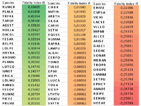
Table 9: Species with high fidelity index to the inter-rows (green on the left), fidelity index close to zero (orange in the middle) and high fidelity index to the rows (red on the right)
Table 10: The F_value, the estimate and the significance concerning the habitat, the production mode and the interaction between both, for the species richness, the abundance, the functional richness (FRic) and the Rao’s quadratic richness. The points (.) indicated a p_value above 0.05, the stars indicated a p_value between 0.05 and 0.01 with a star (*), a p_value between 0.01 and 0.001 with two stars (**) and a p_value under 0.001 with three stars (***). The adjusted R² indicated the contribution of the model to the diversity’s indicators.
Figure 5: Diversity’s indices, i.e. the species richness (a,b), the abundance (c,d), the functional richness (e,f) and the Rao’s quadratic entropy (g,h), according to the area (inter-rows in blue, rows in red), the mode of production called here certification (conventional in orange and organic in green). The horizontal bar of the boxplot represents the median, 50% of the values were located from the 1st quartile
to the 3rd quartile (interquartile range, IQR). Blacks dots are values higher or lower than 1.5 the IQR.
Diversity R² (adjusted) Area Production mode Interaction
Species richness 0.37 162.8/-11.5 *** 1.68/1.34 3.06/2.57 .
Abundance 0.36 127.3/-2.30 *** 17.5/0.98 *** 1.56/0.41
FRic 0.17 50.99/-0.025 *** 2.65/0.0066 0.09/0.0018
The competitors were positively correlated with maximum height, hemicryptophytes (tussock and erected), soil properties and climatic conditions (continentality, trophic level, pH and soil moisture). The stress tolerant species were positively correlated with Ellenberg’s indicators for temperature and for light and negatively to Ellenberg’s indicators for trophic level and for soil moisture.
I.3. Describing the fidelity index to the inter-row by the traits’ variables
The index of fidelity to the inter-rows (IR) ranged from -0.098 for Hedera helix (the species with the highest fidelity to the rows (R)) to 0.44 for the Rumex crispus (the species with the highest fidelity to the IR). Table 9 list the fidelity scores for the more frequent plants based on the presence/absence data. It seemed that there were more species with high fidelity to the IR than species with high fidelity to the R. The species with a high fidelity to the IR were all hemicryptophytes, mainly anemogamous and entomogamous, heliophilous and nitrophilous. The species with high fidelity to the R, which are treated chemically by herbicides, were mainly split in two categories. The first one counted small annuals with short life cycle until March/April and the second one, the woody species like Hedera helix possessing deep roots and waxy leaves giving natural tolerance to herbicides sprays.
The fidelity index to the IR was significantly linked to Ellenberg’s indicators for temperature (cor = -0.16, P = 0.03) and for soil moisture (cor = 0.27, P = 0.0001), axis 2 (cor = -0.15, P = 0.03) and axis 3 (cor = -0.24, P = 0.0008). Based on the trait that contributed the most to axes 2 and 3 (Figure 2, Appendix II), this analysis highlight that the fidelity index to the IR was positively correlated with traits’ combination: high maximum height, high seed mass, late flowering onset and various perennials life forms (geophytes with rhizomes, erected and tussock hemicryptophytes, opposed to therophytes), short flowering duration and low SLA. Based on Grime’s strategies, the fidelity index to the IR was positively linked to competitors and negatively to ruderals.
II.
Influence of environment on weed community (functional) diversity
II.1. Effect of conventional and organic production mode
This part aimed to understand if there was an influence of production mode (organic vs conventional), of the areas (R/IR) and/or their interaction on the weed community diversity. The abundance was the only diversity index showing a significant difference between the production modes (Table 10) with a higher score for organic one (Figure 5). The four diversity indices showed a significant difference between the areas (Table 10) with a higher score for the IR (Figure 5).
II.2. Effect of management practices
In this part, the aim was to test if a classification of vineyard plots into groups with similar management practices can more accurately explain weed community diversity. Based on the three first axes of the PCA (representing 67.8% of the total variability of the practices’ matrix), the Hierarchical Cluster Analysis and the Mantel statistic, we were able to distinguish four groups of plots (Appendix III).
Table 11: F_value of linear models with interaction of the diversity’s indices. The point (.) indicated a p_value above 0.05, the stars indicated a p_value between 0.05 and 0.01 with one star (*), a p_value between 0.01 and 0.001 with two stars (**) and a p_value under 0.001 with three stars (***).
Diversity’s indices Area (rows/inter-rows) Group Interaction
Species richness 18.1 *** 12.4 *** 10.2 ***
Abundance 14.9 *** 8.5 *** 5.6 ***
FRic 4.0 * 7.6 *** 4.2 **
Rao 8.7 ** 3.6 * 4.6 **
Figure 6: Boxplots of the repartition of the four groups depending on the diversity’s indices: Species richness (a), Abundance (b), Functional richness (c) and Rao’s quadratic entropy (d). The inter-rows were represented in dark grey and the inter-rows in pale grey, the group 1 is in yellow, the group 2 in red, the group 3 in green and the group 4 in blue.
Table 12: Linear models given the F_value and the estimate for the four indices of diversity: species richness (S), abundance (Abun), functional richness (FRic) and the Rao’s quadratic entropy (Rao). A compartment in color is significant, green for the positive interactions and yellow for the negative ones. The point (.) indicated a p_value above 0.05, the stars indicated a p_value between 0.05 and 0.01 with one star (*), a p_value between 0.01 and 0.001 with two stars (**) and a p_value under 0.001 with three stars (***). Traits/ Var Date Winter Area R V_100 m
Sand MO CN pH feng famo nherb wir wsr Nton
t_ir Ntont_ sr npm Rainfall S 85.2 5.9 *** 278.6 -10.6 *** 2.6 -0.54 10.9 -1.1 ** 3.6 0.65 . 12.5 -1.3 *** 8.6 -1.2 ** 10.4 -1.2 ** 9.3 1.02 ** Abun 28.4 0.2 *** 213.1 -0.6 *** 14.9 -0.08 *** 5.9 -0.06 * 10.0 0.08 ** 2.2 0.04 15.3 0.08 *** 40.0 -0.2 *** 7.6 -0.08 ** 2.1 0.04 8.3 -0.07 ** 7.5 0.06 ** FRic 90.9 0.02 *** 98.7 -0.03 *** 5.5 0.003 * 16.8 -0.006 *** 4.3 -0.003 * 5.1 0.003 * 2.3 -0.002 Rao 107.5 0.005 *** 93.0 -0.004 *** 10.5 -0.001 ** 16.1 -0.001 *** 9.5 0.001 ** 9.0 -0.001 ** 7.1 0.001 ** 8.6 -0.001 ** 10.7 -0.001 ** 3.1 -0.0004 .