Science Arts & Métiers (SAM)
is an open access repository that collects the work of Arts et Métiers Institute of Technology researchers and makes it freely available over the web where possible.
This is an author-deposited version published in: https://sam.ensam.eu Handle ID: .http://hdl.handle.net/10985/17463
To cite this version :
Jianchang ZHU, Mohamed BEN BETTAIEB, Farid ABED-MERAIM - Numerical investigation of necking in perforated sheets using the periodic homogenization approach - International Journal of Mechanical Sciences - Vol. 166, p.105209 - 2020
Any correspondence concerning this service should be sent to the repository Administrator : archiveouverte@ensam.eu
1
Numerical investigation of necking in perforated sheets using the periodic
homogenization approach
Jianchang Zhu1, Mohamed Ben Bettaieb1,2*, Farid Abed-Meraim1,2 1 Université de Lorraine, CNRS, Arts et Métiers ParisTech, LEM3, F-57000, France
2 DAMAS, Laboratory of Excellence on Design of Alloy Metals for low-mAss Structures, Université
de Lorraine, France
* Corresponding author: Mohamed.BenBettaieb@ensam.eu
Abstract
Due to their attractive properties, perforated sheets are increasingly used in a number of industrial applications, such as automotive, architecture, pollution control, etc. Consequently, the accurate modeling of the mechanical behavior of this kind of sheets still remains a valuable goal to reach. This paper aims to contribute to this effort by developing reliable numerical tools capable of predicting the occurrence of necking in perforated sheets. These tools are based on the coupling between the periodic homogenization technique and three plastic instability criteria. The periodic homogenization technique is used to derive equivalent macroscopic mechanical behavior for a representative volume element of these sheets. On the other hand, the prediction of plastic instability is based on three necking criteria: the maximum force criterion (diffuse necking), the general bifurcation criterion (diffuse necking), and the loss of ellipticity criterion (localized necking). The predictions obtained by applying the three instability criteria are thoroughly analyzed and compared. A sensitivity study is also conducted to numerically investigate the influence on the prediction of necking of the design parameters (dimension, aspect-ratio, orientation, and shape of the holes), the macroscopic boundary conditions and the metal matrix material parameters (plastic anisotropy, hardening).
Keywords:
Perforated sheets; Periodic homogenization; Diffuse and localized necking; Bifurcation analysis; Sensitivity study.2
1. Introduction
Due to their lightness and aesthetic attractiveness, perforated sheets have been increasingly used in various industrial fields, including automotive, architecture, agriculture, pollution control, and mining (IPA, 2015). Additionally, the variety of patterns and perforation shapes makes them quite versatile. To accurately design and manufacture press-formed products, in-depth knowledge of the mechanical behavior and the conditions of occurrence of plastic instabilities in this kind of sheets remains a crucial task for both scientific and technological communities. The theoretical and numerical modeling of the mechanical behavior of perforated sheets has been widely investigated in several previous contributions in the literature. The various developed models have as objectives to predict the geometric distribution of the relevant mechanical fields (stress, plastic strain, …) or to derive an effective (macroscopic) constitutive model representative of the mechanical behavior of the perforated medium as well as the corresponding mechanical parameters (elasticity parameters, anisotropy parameters, hardening parameters). Among these investigations, one can quote the pioneering work of O’Donnell and Langer (O’Donnell and Langer, 1962), who have developed a theoretical method for calculating the stress distribution and effective mechanical properties of perforated plates with triangular penetration pattern. In O’Donnell and Langer (1962), the mechanical behavior of the dense matrix is assumed to be linear elastic. More recently, Krajcinovic et al. (1992) have applied the percolation theory to determine the stress state and distribution in a two-dimensional elastic medium containing randomly distributed circular voids. The effect of plastic behavior of the dense matrix on the effective properties of perforated sheets has been widely studied in several contributions. In these contributions, the effective (macroscopic) plastic behavior has been generally determined by defining a yield criterion and the corresponding evolution of the yield stress (macroscopic hardening). Chen (1993) has performed finite element simulations and experimental tensile tests to propose a yield criterion and the associated flow rules for perforated sheets with circular holes in hexagonal or equilateral triangular patterns. In Chen (1993), both von Mises and Hill’48 yield functions have been used to characterize the plasticity of the dense matrix. A similar methodology has been followed in Baik et al. (1997) to determine a yield criterion for perforated sheets with a uniform triangular pattern of round holes. In the latter contribution, the plastic anisotropy of the metal matrix has been modeled by the von Mises and Hosford yield functions. It should be noted that in the previous works (Chen, 1993; Baik et al., 1997), the classical finite element method has mainly been used to determine the effective mechanical behavior of a representative volume element (RVE) of the studied perforated sheet. Concretely, to build a typical yield function, a monotonically increasing loading combination is applied on the RVE. This loading is assumed to be linear in the macroscopic stress space (the ratio of
3
the major to minor average stresses is kept constant during loading), while the shear stress is set to zero. During this loading, the homogenized stress–strain data are recorded. The yield point is determined from the plot of the effective (macroscopic) equivalent stress as a function of the effective equivalent plastic strain. The numerical modeling of the mechanical behavior of perforated sheets has been significantly improved by coupling the classical finite element analysis to multiscale approaches. These multiscale approaches are based on the concept of substituting a heterogeneous medium with an equivalent macroscopically homogeneous one. In this context, perforated sheets are viewed as heterogeneous media made of two main phases: the hole and the metal dense matrix (which may be itself made of several metallurgical phases). Such a multiscale strategy has been used by several authors to characterize equivalent mechanical behavior of perforated sheets. For instance, van Rens et al. (1998) have used a numerical homogenization approach to determine the initial yield function and its evolution for a RVE of perforated sheets with square pattern of circular holes. More recently, Khatam and Pindera (2011) have employed a finite-volume direct averaging micromechanics (FVDAM) theory to accurately determine the homogenized response of perforated sheets with hexagonal arrays of circular holes, and to establish the relation of homogenized response to yield and limit surfaces. In the current contribution, we have adopted a multiscale strategy to study the mechanical behavior of perforated sheets with periodically distributed holes (in the two directions of the plane of the sheet). Considering this periodic distribution, the periodic homogenization technique (Miehe, 2003) has been used to determine the overall mechanical behavior of one square pattern, which is selected to be the unit cell representative of the studied sheet. It is worth noting that the mechanical behavior of perforated shells and plates has been extensively studied by using the asymptotic homogenization approach in several contributions (Andrianov et al., 2012a, 2012b; Kalamkarov, 1992, 2014; Kalamkarov et al., 2012, Kalamkarov and Kolpakov, 1997). By contrast to the above references, which are mainly focused on the derivation of the macroscopic behavior of perforated thin structures (determination of the effective macroscopic elastic properties…), our contribution aims to investigate the onset of plastic instability in perforated sheets. As such instability usually occurs in the finite strain range, a total Lagrangian framework is adopted to express the assumptions and equations governing the periodic homogenization approach. Within this framework, the deformation gradient (resp. the first Piola–Kirchhoff stress tensor) is used as strain (resp. stress) measure. The periodic homogenization scheme is based on the assumption of spatial periodicity of the microscopic mechanical fields (namely, the microscopic deformation gradient and the microscopic first Piola–Kirchhoff stress) over the boundary of the unit cell. The equations governing the periodic homogenization technique are solved by the finite element method. To achieve this task, a set of python scripts for Abaqus, called Homtools (Lejeunes and Bourgeois, 2011), has been used to easily
4
apply the periodic boundary conditions and to determine the macroscopic first Piola–Kirchhoff stress tensor associated with the prescribed macroscopic deformation gradient.
Despite the large number of contributions dedicated to the modeling of the mechanical behavior of perforated sheets and to the determination of their effective macroscopic properties (effective elastoplastic parameters, shape of the macroscopic yield surface and its evolution), theoretical investigations on the necking and formability of perforated sheets are still seldom and not very extensive. It is however well recognized that the initiation of plastic instability in this kind of sheets is essentially dependent on the mechanical behavior of the dense matrix and on the morphology (size and form) of patterns and holes. In the majority of past studies related to this particular issue, perforated sheets are considered as thin media containing periodic array of cylindrical voids. Tvergaard (1981) is one of the first authors who extensively studied the onset of plastic strain localization in voided sheets under several mechanical states, such as uniaxial and biaxial plane-strain tension. In the latter reference, plastic strain localization is viewed as a bifurcation from the fundamental solution path, and Hill’s theory of uniqueness (Hill, 1958) has been used to numerically predict bifurcation. To apply this analysis, the incremental form of the virtual work principle has been established on the basis of the incremental equilibrium equations. At each stage of the loading history, an approximate solution to this incremental form has been obtained by the finite element method. Bifurcation occurs when the determinant of the global stiffness matrix vanishes. In Tvergaard (1981), the limit strains given by bifurcation theory have been compared with their counterparts obtained by the maximum nominal traction criterion (diffuse necking criterion). More recently (Tvergaard, 2015), the previous study has been extended to void-sheets subjected to simple shear and pure shear states. It is to be noted that Tvergaard’s investigations (Tvergaard, 1981; Tvergaard, 2015) have been restricted to the following particular choices and assumptions: only some specific strain and stress states are studied, the form of voids is taken to be solely circular, and the plane-strain condition is assumed in the thickness direction of the sheet. In addition to these investigations, the necking occurrence in perforated sheets has also been analyzed through the classical concept of forming limit diagrams (FLDs). As the studied sheets are assumed to be thin, FLD predictions have been legitimately based on the plane-stress assumption in the thickness of the sheet (Hutchinson et al., 1978). Furthermore, a wide range of strain paths (from uniaxial tension state to equibiaxial tension state) is covered when the FLD approach is used. The concept of forming limit diagrams has been first applied to perforated sheets in Iseki et al. (1989). In this investigation, a diffuse necking criterion has been used to predict the onset of necking. According to this criterion, the necking limit is reached when the product of external force and displacement rate reaches a maximum value. The effect of hole shape (circular, elliptical, square) on the formability limit has been particularly highlighted in Iseki et al. (1989). It has been found from this study that
5
perforated sheets with square holes have the best formability limit. Iseki’s formability criterion (Iseki et al., 1989) has been subsequently used by Chiba et al. (2015) to predict the FLDs of perforated aluminum sheets with square holes. In this analysis, both phenomenological material models (based on Hill’48 and von Mises yield functions) and a crystal plasticity model have been used to describe the mechanical behavior of the dense matrix. In the above-cited contributions (Chiba et al., 2015; Iseki et al., 1989; Tvergaard, 1981; Tvergaard, 2015), finite element analyses have been combined with the different necking criteria to predict the onset of necking. In the present investigation, we have coupled the periodic homogenization approach with some diffuse and localized necking criteria to predict the forming limits of perforated sheets. The onset of diffuse necking is predicted by the maximum force criterion (Considère, 1885) and the general bifurcation criterion (Drucker, 1950, 1956; Hill, 1958). As to localized necking, its occurrence is determined by the loss of ellipticity criterion (Rudnicki and Rice, 1975). To apply both bifurcation criteria, the analytical tangent modulus, which relates the macroscopic first Piola–Kirchhoff stress rate to the macroscopic deformation gradient rate (as a total Lagrangian formulation is adopted), needs to be determined. To compute this tangent modulus, we have used the condensation technique initially developed in Miehe (2003). The condensation method as well as the different necking criteria have been implemented in a set of Python scripts.
A brief outline of the present paper is as follows:
Section 2 details the modeling of the mechanical behavior of the perforated sheets.
Section 3 gives the main lines of the adopted necking criteria.
The numerical results of the current study are reported in Section 4. Our numerical results are firstly compared with the numerical predictions of Tvergaard (1981). Secondly, a sensitivity study is conducted to analyze the effect of several mechanical and design parameters on the shape and the level of forming limit diagrams.
Section 5 closes our contribution by summarizing some conclusions and future work.
Notations, conventions and abbreviations
Microscale (resp. macroscale) variables are denoted by lowercase (resp. capital) letters. Vectors and tensors are indicated by bold letters and symbols. By contrast, scalar parameters
and variables are designated by thin and italic letters and symbols.
Einstein’s convention of implied summation over repeated indices is adopted. The range of free (resp. dummy) index is given before (resp. after) the corresponding equation.
a time derivative of a. aper periodic field a.
6
a b. inner product of a and b. a b: double contraction of a and b. a b tensor product of a and b. aT transpose of a.
0
divx a
divergence of field a with respect to the initial position x0
.
a
the virtual counterpart of field
a.
2. Modeling of the mechanical behavior of perforated sheets
2.1. Multiscale transition problem
We consider a thin perforated sheet with a large number of holes, which are periodically distributed in the two directions of the plane of the sheet as depicted in Fig. 1a. This perforated sheet may be viewed as a heterogeneous medium made of two main phases: the hole and the metal matrix. Consequently, the mechanical behavior of this perforated sheet could be modeled by using a multiscale scheme. The metal matrix is assumed to be homogeneous, as microscopic heterogeneities between the different metallurgical phases are neglected in this study. The first step in the application of this multiscale process consists of the selection of a RVE, such that duplicating it provides sufficient accuracy for representing the material larger scales. In the current contribution, we have chosen a RVE with square pattern containing a unique hole located in the center of the RVE (Fig. 1b). The second step concerns the choice of the most relevant multiscale scheme to determine the homogenized behavior of this RVE. Considering the periodicity of the hole arrangement, the periodic homogenization technique (Miehe, 2003) is selected for this purpose. The use of this homogenization technique allows us to replace the heterogeneous RVE (called also unit cell in the context of periodic homogenization) by an equivalent homogenized medium with the same effective mechanical properties (Fig. 1c).
(a) (b) (c)
7
In what follows, capital (resp. small) letters and symbols will be used to denote macroscale (resp. microscale) quantities and variables. The periodic homogenization scheme is defined by the following main equations:
The periodicity conditions, where the microscopic deformation gradient f is additively decomposed into its macroscopic counterpart and a fluctuation gradient fper:
, per
f F f (1)
where fper is periodic over the boundary of the unit cell (in its initial configuration). As a consequence of its periodicity, the volume average of fper is equal to zero:
0 0 0 1 f 0
per V dV V , (2)where V is the initial volume of the unit cell. 0
By spatial integration of Eq. (1), the current position x
of a microscopic material point is
expressed as a function of its initial position x and a periodic displacement field 0per u : 0 . per x F x u (3)
The microscopic first Piola–Kirchhoff stress tensor p is also assumed to be periodic over the boundary of the unit cell in its initial configuration. This periodicity also requires the anti-periodicity of the stress vector p n 0 (where n is the outer normal on the boundary of 0 V ). 0
The averaging relations, which allow relating the macroscopic deformation gradient F and the macroscopic first Piola–Kirchhoff stress tensor P to their microscopic counterparts f x and
p x :
0 0 0 0 0 0 1 1 ; V dV V dV V V
F f x P p x , (4) The constitutive relation at the macroscopic scale, relating the rate of the macroscopic first Piola–Kirchhoff stress tensor P to the rate of the macroscopic deformation gradient F through the macroscopic tangent modulus PK1
(
Ji et al., 2013; Nguyen and Waas, 2016
):
= PK1:
P F . (5)
The microscopic static equilibrium equation in the absence of body forces:
0
8
The constitutive relations that describe the mechanical behavior of the dense matrix, which will be detailed in Section 2.2.
2.2. Constitutive relations at the microscale level
As the metal matrix is assumed to be homogeneous, a phenomenological constitutive framework is sufficient to describe the mechanical behavior of a microscopic material point from this matrix. To simplify the notations in the following developments, reference to the current position of the microscopic material point x in the different mechanical fields will be omitted. Perforated sheets are generally manufactured from cold-rolled products, which exhibit non negligible plastic anisotropy. Hence, a plastically anisotropic and rate-independent framework is chosen to model the mechanical behavior of the metal dense matrix. To develop the constitutive equations governing the mechanical behavior of the dense matrix, it is more convenient to use an Eulerian formulation. In this formulation, the velocity gradient l and the Cauchy stress tensor are used as strain and stress measures. These tensors are related to their Lagrangian counterparts f and p by the following classical relations:
1
. ; . with det ,
lf f pjσ fT j f (7)
where fT denotes the transpose of the inverse of tensor f .
The microscopic velocity gradient l is additively decomposed into its symmetric and skew-symmetric
parts, denoted d and w , respectively:l d w. (8)
To satisfy the objectivity principle (i.e., frame invariance), objective derivatives for tensor variables should be used. A practical approach, used to ensure frame invariance while maintaining simple forms of the constitutive equations, consists in reformulating these equations in terms of rotation-compensated variables. In the present work, a co-rotational approach based on the Jaumann objective rate is used. Accordingly, tensor quantities are expressed in a rotating frame so that simple material time derivatives can be used in the constitutive equations. The rotation r of this rotating frame, with respect to the fixed one, is derived from the spin tensor w (skew-symmetric part of l ) by the following relation:
. T
r r w . (9)
In the remainder of the current section (Section 2.2), all tensor variables will be expressed in the rotating frame (called co-rotational frame), that is to say, using rotation-compensated variables. Consequently, time derivatives are involved in the constitutive equations, making them identical in form to a small-strain formulation.
9
The strain rate d is itself split into its elastic part d and plastic part e d :p
e p
d d d . (10)
The stress rate is described with a hypoelastic law: : e e
c d
, (11)
where c denotes the fourth-order elasticity tensor. Here, elasticity is assumed to be isotropic and is e defined by two material parameters: the Young modulus E and the Poisson ratio .
The plastic strain rate d is assumed to be normal to the yield surface, and the following normality p law is adopted:
p
d
, (12)
where denotes the plastic multiplier, and is the yield function defined as the difference between the equivalent stress eq
and
the microscopic yield stress y. In the current contribution, the Hill’48 criterion is used as equivalent stress measure (Hill, 1948), while hardening is assumed to be isotropic and is modeled by the Swift law. Consequently, eq and y are defined by the following expressions:
0
: : p n
eq y K eq
H , (13)
where:
K , 0 and n are hardening parameters.
p
eq
is the equivalent plastic strain.
H is the Hill’48 orthotropic matrix, whose components are expressed in terms of three Lankford coefficients (r r0, 45,r ) that measure the degree of plastic anisotropy. 90
The activation of the plastic deformation is governed by the well-known Kuhn–Tucker constraints:
eq y
0 0 0 . (14)
The Cauchy stress rate is related to the strain rate d by the elastoplastic continuum tangent matrix ep
c :
ep
c d
. (15)
The expression of this elastoplastic tangent modulus can be obtained by combining the different constitutive equations (8)–(15). One can obtain after classical computations the following expression for c (ep Haddag et al., 2007):
10
: : : : e e ep e y e p eq c c c c c . (16)2.3. Numerical implementation of the multiscale transition scheme
The periodic homogenization equations have been solved by the finite element method. To achieve this task, we have used the toolbox Homtools developed by Lejeunes and Bourgeois (2011). This toolbox consists of a set of python scripts for Abaqus that greatly simplify and automatize the determination of homogenized characteristics of heterogeneous materials and structures. Homtools integrate some GUIs that permit to easily define the periodic boundary conditions and the average loadings in the CAE. As a first step in solving this problem, the unit cell is discretized by finite elements (Fig. 2). 3D finite elements (C3D20) have been used in this work, in spite of the small thickness of the studied sheets. As the current tool is used to predict forming limit diagrams, the unit cell is submitted to biaxial stretching along the 1 and 2 directions, while under a plane-stress state in the third direction (Fig. 2). This loading is represented by the following generic macroscopic fields:
11 22 0 0 ? ? ? 0 0 ; ? ? ? ? ? ? 0 0 0 F F F P , (17)
where the components denoted by ‘?’ are the unknown components that need to be determined. The unit cell is submitted to the following boundary conditions:
On the boundary surfaces B1 and B1
: a reference point (following the Abaqus terminology) is created to apply the components F11, F12( 0) and F13( 0) of the macroscopic deformation
gradient F . Furthermore, for the displacement components at the two corresponding nodes x 0q
and x with identical coordinates in 2 and 3 directions on surfaces 0q B1
and B1
, the following constraint equation is imposed:
0q 0q 0q 0q
u u F x x . (18)
Constraint equation (18) can be easily obtained by combining Eq. (3) and the periodic condition between the two corresponding nodes.
11
On the boundary surfaces B2
and B2
: a reference point is created to apply the components
21( 0)
F , F22 and F23( 0) of F . Furthermore, a periodic constraint, similar to the one
imposed to the nodes of surfaces B1
and B1
, is applied.
On the boundary surfaces B3 and B3: the macroscopic stress normal to these surfaces is taken to be equal to zero (P33 0).Fig. 2. Finite element discretization and boundary conditions applied to the unit cell.
As the finite element method is used to solve the periodic homogenization relations, the equations governing this method shall be given here quite briefly. To this end, the equilibrium equation (6) could be equivalently rewritten using the rate of the first Piola–Kirchhoff stress tensor:
0
divx p 0. (19)
The formulation of the finite element equations is based on the virtual work principle. To formulate this principle, let us integrate the scalar product between Eq. (19) and the virtual velocity field u over the volume of the unit cell in its initial configuration V : 0
0
0 0
Vdiv . dV 0
x p u . (20)On the other hand,
0divx p.u can be additively decomposed in the following form:
0 0 0 divx p. u divx p . u p: u x . (21)12
0 0 0 0 div . : 0 V dV
x u p u p x . (22)The Gauss theorem allows us to rewrite a volume integral according to:
0 0 0 0 0 0 . a n a x
V dV
S dS , (23)where a is any continuous scalar, vector, or tensor function and n is the outward normal to the 0
surface S . By applying the Gauss theorem, it is easy to transform Eq. (22) into the following form: 0
0 0 0 0 0 : u . p u t x
V dV
S dS , (24)where S is the boundary of the unit cell in the initial configuration, and t is the rate of the traction 0
vector, equal to p n , at points . 0 x0S with outward unit normal vector 0 n . 0
Using the developments reported in Appendix A, one can easily prove that:
0 0 0 0 : u : p P F x
V dV V . (25)On the other hand, one can demonstrate after some mathematical developments the following equality (Ji et al., 2013): 0 0 0 0 0 : u : 2 : ( ) : ( ) d p τ d τ d d τ l l x
J T V dV V V , (26)where τ is the Jaumann derivative of the Kirchhoff stress tensor. The establishment of this equality J is necessary, as the virtual work principle is formulated in Abaqus in the form of the right-hand side of Eq. (26) (Abaqus, 2014). Comparing Eqs. (25) and (26), one can see that:
0 0 0 : 2 : ( ) : ( ) d : τ d τ d d τ l l P F
J T V V V . (27)As shown in Debordes (1986), Miehe and Bayreuther (2006) and Temirez and Wriggers (2008) for the classical periodic homogenization technique within a total Lagrangian formulation, Eq. (27) enables, in the finite element process, to treat the macroscopic deformation gradient rate F as macroscopic degrees of freedom associated with the nodal forces V P . Practically, the application of macroscopic 0
loading within Abaqus is ensured by the reference point technique (Lejeunes and Bourgeois, 2011). The macroscopic force R1 applied on the boundary surfaces B1
and B1
is obtained by multiplying the component P11 by the initial surface S of boundaries 01 B1
or B1
13
1 11 01
R P S . (28)
A similar relationship can be defined between the force R2 applied on B2
and B2
and P22.
2.4. Computation of the macroscopic tangent modulus
The application of the bifurcation criteria discussed in Section 1 (see also Section 3 for more details) requires the computation of the macroscopic tangent modulus PK1 introduced in Eq. (5). To determine this tangent modulus from the finite element outputs, we have developed a set of Python Scripts. The condensation technique proposed by Miehe (2003) is followed for the development of these scripts. The main steps of this technique will be outlined in the following developments. Further information about this technique can be found in Miehe (2003).
Step 1: at the convergence of the finite element method, Abaqus offers the possibility to save the elementary stiffness matrices K in a ‘.mtx’ file by using the command ‘Element Matrix el Output’. A classical assembly procedure has been implemented to determine the global stiffness
matrix K from the elementary ones K and by taking into account the connectivity of the el
different nodes of the mesh:
1 el Nel el el K K , (29)
where Nel refers to the total number of finite elements in the mesh.
Step 2: the nodes of the mesh are partitioned into two sets (Fig. 2): set b made of nodes located on the boundary surfaces B1 B1 B2 B2
where periodicity constraints are applied (M nodes), and set a which is composed of the other nodes of the mesh (N nodes). By using this partition, the lines and columns of the global stiffness matrix K are rearranged (permuted) to obtain the following decomposition:
aa ab ba bb K K K K K . (30)
Step 3: matrices S and Q are computed by following the numerical procedure detailed in Appendix B.
Step 4: the macroscopic tangent modulus is computed by using the following relation:
1 1 1 0 1 . . . . PK1 T T bb ba aa ab V Q S K K K K S Q . (31)14
The constitutive equations used to model the mechanical behavior of the dense matrix have been integrated by using an Euler explicit algorithm and implemented as a UMAT subroutine in Abaqus. As the integration algorithm is explicit, the consistent elastoplastic tangent modulus used to construct the stiffness matrix K coincides with the analytical one given by Eq. (16), as explained in Simo (1998). As demonstrated in Temizer and Wriggers (2008), the condensation technique allows us to obtain an analytical macroscopic tangent modulus if the microscopic one, used to compute the global stiffness matrix K , is itself analytical. Consequently, PK1 is an analytical tangent modulus, which can be used without any modification in the subsequent bifurcation analyses.
3. Necking criteria
To predict the occurrence of necking in thin perforated sheets, and represent the prediction results in terms of forming limit diagrams, the applied macroscopic deformation gradient given in Eq. (17) is defined by the following in-plane components:
11 22
11 e ; 22 e with 22 11
E E
F F E E . (32)
To cover the whole range of strain paths, relevant for the plot of forming limit diagrams, the strain-path ratio is varied between 1/ 2 (uniaxial tensile state) and 1 (equibiaxial tensile state).
The periodic homogenization technique is used to determine the macroscopic first Piola–Kirchhoff stress tensor P and the corresponding analytical tangent modulus PK1 associated with the prescribed macroscopic deformation gradient. To predict the onset of necking in the unit cell, P and PK1 are used as inputs for three necking criteria: the Maximum Force Criterion (MFC), the General Bifurcation Criterion (GBC), and the Rice Bifurcation Criterion (RBC). These plastic instability criteria will be briefly presented in the following Sections (3.1; 3.2 and 3.3).
3.1. Maximum Force Criterion
Swift (1952) proposed a diffuse necking condition for stretched metal sheets submitted to biaxial loading, as depicted in Fig. 2. This condition can be mathematically expressed as:
1 0 and 2 0
R R . (33)
Condition (33) suggests that diffuse necking occurs when components R1 and R2 reach their maximum values simultaneously. However, the satisfaction of this simultaneous condition is only possible for two particular strain paths (uniaxial and equibiaxial strain paths), as it has been experimentally and theoretically demonstrated in Habbad (1994) and Abed-Meraim et al. (2014).
15
Accordingly, to be able to predict the onset of diffuse necking for the whole range of strain paths, we only consider the first condition in Eq. (33), namely:
R10. (34)
As the component P11 of tensor P is proportional to force R1, condition (34) can be equivalently rewritten as:
11 0
P . (35)
3.2. General Bifurcation Criterion
Diffuse necking is also predicted by the general bifurcation criterion (GBC). This criterion states that plastic instability occurs when the second-order work vanishes (Drucker, 1950, 1956; Hill, 1958). According to the GBC, diffuse necking is predicted when at least one eigenvalue of the symmetric part of PK1 (called hereafter PK1
sym ) becomes negative. Further details about the development of this criterion are provided in Bouktir et al. (2018).
3.3. Rice’s Bifurcation criterion
In the approach proposed by Rudnicki and Rice (1975), material instability corresponds to a bifurcation associated with admissible jumps for strain and stress rates across a localization band, as illustrated in Fig. 3. In a Lagrangian formulation, the kinematic condition for the strain rate jump writes:
0 0
F F F , (36)
where F is the jump of the velocity gradient field F across the discontinuity band, while 0 is the
jump vector, and 0 is the unit vector normal to the localization band in the initial configuration. On the other hand, the continuity condition for the force equilibrium across the band is expressed as:
. 0
P 0 . (37)
The combination of Eqs. (36) and (37) with the macroscopic constitutive law (5) leads to the following equation:
: 0
. 0PK1
0 0 , (38)
16
0 0
0 1, 2,3: 0, , , 1, 2,3 PK1 j ijkl l k i j k l . (39)By introducing matrix
, defined as the transpose of matrix
PK1by permutation of the first two indices ( ijkl jiklPK1), condition (39) can be rewritten as follows:
0 0
01, 2,3 : 0, , , 1, 2,3
j i ijkl l k i k l , (40)
which is equivalent to:
0. . 0
. 0 0 . (41)Tensor 0. . 0
is the so-called acoustic tensor. As long as this tensor is invertible, the jump vector
0 remains equal to zero, thus precluding any discontinuity (bifurcation) in the deformation field.
However, when the acoustic tensor becomes singular, there exists non-zero jump vectors that satisfy Eq. (41), and this can be seen as indicator of effective bifurcation. Therefore, strain localization occurs when the acoustic tensor is no longer invertible:
0 0
det . . 0. (42)
The bifurcation criterion given by Eq. (42) is implemented in the set of Python codes by following the algorithm developed in Ben Bettaieb and Abed-Meraim (2015).
Fig. 3. Illustration of the Rice bifurcation criterion.
4. Results and discussions
4.1. Results for homogeneous unit cell
To provide a first validation to the developed numerical tools, attention is confined here to the prediction of the occurrence of necking in a homogeneous unit cell (without holes). For this simulation,
17
the mechanical behavior is assumed to be plastically isotropic, following the von Mises yield function. In this context, the Lankford coefficients r , 0 r and 45 r used in the Hill’48 yield function are set to 1. 90
Elastic and isotropic hardening parameters (Eq. (13)) are reported in Table 1. These parameters correspond to the aluminum alloy AA5052-O.
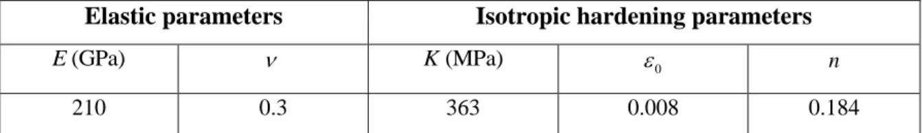
Table 1. Elastic and hardening material parameters.
Elastic parameters
Isotropic hardening parameters
(GPa)
E K (MPa) 0 n
210 0.3 363 0.008 0.184
The prediction of the onset of necking using the above-described diffuse and localized necking criteria is illustrated in Fig. 4 for three particular strain paths: ,
, and
. In Fig. 4a, the evolution of the component P11 is plotted as a function of E11 (Ln F
11 ). For MFC, the moment when P11 reaches its maximum value is considered as indicator of the onset of diffuse necking. For the three strain-path ratios considered, the corresponding stress–strain curves are clearly distinct, but the maximum values for P11 are reached at the same strain level, which is equal to n0 (0.176). Theevolution of the cubic root of the determinant of the symmetric part PK1sym
of
PK1is plotted as a function of E11 in Fig. 4b. The onset of necking starts, according to the GBC, when the smallest eigenvalue of PK1sym vanishes, or in an equivalent way, when PK1sym becomes singular (as symPK1 is positive definite before it becomes singular). As clearly shown in this figure, the predicted limit strains
11
E are strictly the same (equal to n0 0.176) for the three different strain-path ratios considered.
The predictions based on RBC are reported in Fig. 4c, where the evolution of the cubic root of the minimum of the determinant of the acoustic tensor, over all possible orientations 0
for the
localization band, is plotted as a function of E11. It can be seen that, irrespective of the selected strain path, the minimum of that determinant abruptly drops during the transition from elastic to plastic regime. This determinant vanishes for the strain-path ratios and at strain levels equal to 2 n
0
and n0, respectively. By contrast, this determinant remains strictly positive, even forvery large strain levels, for the equibiaxial tension state (). Consequently, localized necking cannot be predicted by RBC for this particular strain-path ratio.
18
0.0 0.1 0.2 0.3 0.4 0 50 100 150 200 250 300 11 0.5 0 1 P11 (MPa) maximum 0.0 0.1 0.2 0.3 0.4 0 1x10⁵ 2x10⁵ 3x10⁵ 4x10⁵
11 0.5 0 1
1 3det PK sym (a) (b) 0.0 0.1 0.2 0.3 0.4 0 1x10³ 2x10³ 3x10³ 11 0.5 0 1
1/3 0 0 Min det . . (c)Fig. 4. Prediction of necking, for three particular strain-path ratios, using the different necking criteria:
(a) MFC; (b) GBC; (c) RBC.
Fig. 5 provides the FLDs predicted by using the three different necking criteria. As can be seen, the forming limit curve given by MFC reveals to be a horizontal line, which also coincides with the predictions given by GBC for the three particular strain-path ratios: ; , and (see, e.g., Abed-Meraim et al., 2014). The RBC is able to determine limit strains at localized necking only in the range of negative strain-path ratios. In the latter range, the FLD takes the form of a straight line,
19
along which E11
is equal to
n0
/ 1
. This result may be viewed as an extension of the results demonstrated for the particular case of rigid-plastic behavior. Indeed, the adopted elastoplastic behavior model can be reduced to a rigid-plastic one by setting 0 to 0. In this limiting case ofrigid-plasticity, Hill (1952) has demonstrated that E11
is equal to n/
1
in the left-hand side of the FLD. This classical result has also been confirmed by the recent numerical investigations reported in Ben Bettaieb and Abed-Meraim (2015). For the positive strain-path ratios, the limit strains predicted by RBC are so unrealistically high that they cannot be represented in Fig. 5. It is also clearly shown from Fig. 5 that the three necking criteria provide the same limit strain for the plane-strain state ( ). As a preliminary conclusion, the results given in Fig. 5 represent a first partial validation for the developed numerical tools.-0.2 -0.1 0.0 0.1 0.2 0.0 0.1 0.2 0.3 0.4 22 MFC GBC RBC 11 n
Fig. 5. FLDs for a homogeneous sheet (without holes), as predicted by MFC, GBC, and RBC.
4.2. Comparison with Tvergaard’s results
To further validate the developed numerical approach, our numerical predictions have been compared with those published in Tvergaard (1981). To this aim, our numerical tools have been slightly modified and adapted to be conformal with the simulations performed in Tvergaard (1981). For instance, the plane-strain condition is applied in the thickness direction of the sheet, instead of the plane-stress condition commonly adopted so far. Accordingly, the component F is set to 1 all along 33
20
these comparisons coincide with those considered in Tvergaard (1981). In these comparisons, three different loading states have been considered:
Uniaxial tension state: for this loading, the component P22 is set to 0 (Fig. 6). Consequently,
22
F is left free. The loading is applied in direction 1, where component F11 increases monotonically from 1 (which corresponds to E110) to 2.
Plane-strain tension state: for this loading, the component F22 is set to 1 (Fig. 6). Consequently,
22
P is left free, and component F11 increases monotonically from 1 (which corresponds to
11 0
E ) to 2.
Proportional in-plane stressing: for this loading, the ratio P22P11 of the in-plane components of
the first Piola–Kirchhoff stress tensor is set to 2 (Fig. 6). To apply this loading, component F22
increases monotonically from 1 to 2. The application of this proportional in-plane stressing has required further numerical developments. Indeed, the toolbox Homtools used to apply the macroscopic boundary conditions allows us to easily manage strain-driven boundary conditions. However, for stress-driven boundary conditions, some improvements and extensions are needed. In fact, the application of proportional stressing has been made possible by implementing in Abaqus a procedure based on the coupling of the Homtools and the user-subroutine *MPC (Multi-point constraints). The use of the *MPC subroutine allows us to update the value of component F11 in order to ensure that ratio P22P11 remains equal to 2 during the loading. The
interested reader may refer to Wong and Guo (2015) or Guo and Wong (2018) to better understand how proportional stressing is applied on the unit cell. The new results further confirm the previous and current trends showing the perfect agreement between our numerical predictions and those obtained in Tvergaard (1981).
21
Fig. 6. Initial unit cell used for the comparisons with Tvergaard’s results.
The comparisons between our predictions (in black color) and Tvergaard’s results (in green color) are given in Fig. 7. In this figure, the component P11 normalized by the initial yield stress is plotted as a
function of E11. To analyze the effect of the hole radius on the instability predictions (such as shear band bifurcation), four values for the ratio R0/ A0 are taken (Fig. 6): 0 (which corresponds to
homogeneous unit cell); 0.175; 0.25 and 0.375. From Fig. 7, the following conclusions can be drawn: The plots in Fig. 7 show that the level of the maximum stress P11 is significantly reduced when
increasing the hole diameter. This observed general trend is common to all of the simulations and for both loading situations (i.e., uniaxial tension state, and plane-strain tension state). All of our predictions agree very well with those published in Tvergaard (1981). Indeed, the
11 11
P E curves are perfectly superposed. Furthermore, the bifurcation points that we predict here by using the RBC are identically the same as those predicted in Tvergaard (1981) based on bifurcation theory with instability modes in the form of shear band localization.
For the uniaxial tensile state (Fig. 7a), the strains corresponding to the maximum nominal stress and those associated with bifurcation exhibit opposite evolution with the increase of the ratio
0 0
R / A . Indeed, while the strains corresponding to the maximum nominal stress increase when increasing the void volume fraction, the opposite trend is observed for the bifurcation critical strains.
For the plane-strain tension state (Fig. 7b), when the void volume fraction is set to zero (i.e., homogeneous sheet), the nominal stress does not reach a maximum, and also bifurcation is not predicted. In this case, the strain components E22 and E remain equal to 0 and the sheet is 33
22
deformed with a very small volume change, which is entirely due to elastic compressibility (as plastic deformation is taken to be without volume change). Consequently, a very important stress P11 is required to slightly deform the sheet, and this stress level cannot decrease. For the other ratios (R0/A0 0), maximum nominal stress and bifurcation are more easily reached, as
the volume change of the perforated sheet is allowed by the evolution of the hole volume. For this plane-strain tension state, maximum nominal stress occurs simultaneously with bifurcation when R00.
The results provided in Fig. 7c show that bifurcation cannot be reached for homogeneous sheet (i.e., when ratio R0 /A0 is set to zero) with P22P112 . This result is quite expectable
considering the fact that for this loading, the strain-path ratio is positive (but not constant). For the other unit cells, the limit strains at bifurcation decrease when the hole radius increases. On the other hand, the strains corresponding to the maximum nominal stress are less sensitive to the hole radius, as shown in Fig. 7c.
0.0 0.1 0.2 0.3 0.4 0.5 0.6 0.7 0.0 0.5 1.0 1.5 R0/A0 R0/A0 11 , Maximum , Bifurcation P11/y0 R0/A0 R0/A0 0.00 0.02 0.04 0.06 0.0 0.5 1.0 1.5 2.0 2.5 3.0 R0/A0 R0/A0 11 , Maximum , Bifurcation P11/y0 R0/A0 R0/A0 (a) (b)
23
0.00 0.02 0.04 0.06 0.08 0.0 0.5 1.0 1.5 2.0 2.5 3.0 R0/A0 R0/A0 11 , Maximum , Bifurcation P11/y0 R0/A0 R0/A0 (c)Fig. 7. Comparisons between the current numerical predictions and Tvergaard’s results (in
green color): (a) Uniaxial tension state; (b) Plane-strain tension state; (c) Loading with proportional in-plane stressing P22P112.
4.3. Sensitivity study
In this section, a sensitivity study is conducted to analyze the effect of several design and mechanical parameters on the onset of necking in perforated sheets. When not explicitly specified, the material parameters of the dense matrix are the same as those given in Table 1. A preliminary sensitivity analysis has been performed to investigate the influence of the selected finite element mesh on the necking predictions. The choice of mesh discretization has been mainly dictated by seeking good compromise between the CPU time required for the computations and the accuracy of the predictions. For the sake of conciseness, the details of this preliminary study are not discussed in the current paper.
4.3.1. Effect of the hole radius
In this subsection, the hole is assumed to be initially circular and the influence of its initial radius R 0
on the forming limit diagrams is analyzed (Fig. 8). The results of this analysis are shown in Fig. 9. Contrary to the case of zero void volume fraction (i.e., homogeneous unit cell without holes, see Fig. 5), localized necking for perforated unit cell is predicted at realistic (finite) limit strains, even in the range of positive strain-path ratios (see right-hand side of the FLDs in Fig. 9c). Indeed, the presence of holes induces some softening, which allows promoting the occurrence of localized necking (Tvergaard,
24
1981; Koplik and Needleman; 1988). Clearly, the necking limit strains decrease on the whole when increasing the size of the holes, which corresponds to larger void volume fraction. As clearly shown in Fig. 9, the effect of the hole radius on the necking limit strains is much more pronounced in the range of positive strain-path ratios. This common trend, which is observed for the three adopted necking criteria (see Fig. 9), is directly attributable to the hole growth, which is mainly dependent on the applied loading path as shown in Fig. 10. To further explain this point, let us introduce the surface growth factor S S S0
, with
S and S denoting the initial and current hole surface in the plane of 0the sheet, respectively. One can easily derive the following expression for S :
1 11
0 e E 1 S S . (43)Hence, the surface growth factor increases with the strain-path ratio (and also with the triaxiality factor). For negative strain-path ratios (especially near the uniaxial tensile state, as illustrated in Fig. 10b), S is relatively small and the loading path is characterized more by a change in the hole shape than a change in the hole surface. By contrast, for equibiaxial tensile state, the hole remains circular and the loading path exhibits the largest surface growth factor (Fig. 10c).
(a) (b) (c)
Fig. 8. Unit cells with different circular hole initial radii: (a) R0/A00.1; (b) R0/A00.2; (c)
0/ 0 0.5
25
-0.10 -0.05 0.00 0.05 0.10 0.15 0.00 0.05 0.10 0.15 0.20 22 R0/A00.1 R0/A00.2 R 0/A00.5 11 -0.10 -0.05 0.00 0.05 0.10 0.15 0.00 0.05 0.10 0.15 0.20 22 R0/A00.1 R0/A00.2 R 0/A00.5 11 (a) (b) -0.10 -0.05 0.00 0.05 0.10 0.15 0.00 0.05 0.10 0.15 0.20 22 R0/A00.1 R0/A00.2 R0/A00.5 11 (c)26
(a) (b) (c)
Fig. 10. Schematic evolution of the unit cell: (a) Initial configuration; (b) Current
configuration for 0.5; (c) Current configuration for 1.
4.3.2 Effect of the elliptical hole aspect ratio
It is expected that the hole shape has a significant impact on the mechanical behavior and on the development of necking in perforated sheets. To investigate this aspect, our interest is firstly centered on perforated sheets with elliptical holes. We assume that the minor (resp. major) axis of the hole is aligned with the direction of major (resp. minor) strain E11 (resp. E22), as illustrated in Fig. 11. The initial hole shape is characterized by the initial aspect ratio b0/a , where 0 b (resp. 0 a ) is the major 0
(resp. minor) radius of the hole. In the current simulations, we have used three different values for the ratio b0/a : 1 (which corresponds to a circular hole), 2 and 3 (see 0 Fig. 11). The initial radii a and 0 b 0
are determined in such a way that the hole initial surface is the same for the three different configurations. From Fig. 12, it is clearly shown that the necking limit strains decrease with an increase in the initial aspect ratio b0/a . This result also confirms the trends observed in several 0
pioneering studies, devoted to 3D voided materials and focused on some particular loading paths, which state that void-induced softening is mainly dependent on the ellipsoidal void aspect ratio (see for instance, Pardoen and Hutchinson, 2000; Keralavarma and Benzerga, 2010). These studies have revealed that the increase in void aspect ratio induces accelerated void growth, thus resulting in earlier occurrence of softening.
27
(a) (b) (c)
Fig. 11. Unit cells with different elliptical hole initial aspect ratios: (a) b0/a01; (b)
0/ 02 b a ; (c) b0/a03. -0.10 -0.05 0.00 0.05 0.10 0.15 0.00 0.04 0.08 0.12 22 b0/a01 b0/a2 b0/a3 11 -0.10 -0.05 0.00 0.05 0.10 0.15 0.00 0.04 0.08 0.12 22 b0/a01 b 0/a02 b0/a03 11 (a) (b)
28
-0.10 -0.05 0.00 0.05 0.10 0.15 0.00 0.04 0.08 0.12 22 b0/a1 b0/a02 b0/a03 11 (c)Fig. 12. Effect of the hole aspect ratio on the FLDs predicted by: (a) MFC; (b) GBC; (c) RBC.
4.3.3. Effect of the elliptical hole orientation
In the current subsection, the effect of the elliptical hole orientation on the necking predictions is investigated. To this end, the initial orientation 0, defined by the angle between the major axis of the
hole and the major strain direction, is varied with three values considered for 0: 0° (Fig. 13a), 45°
(Fig. 13b) and 90° (Fig. 13c). Note that the initial shape and aspect ratio of the hole are kept the same for all of the simulations in this subsection. By analyzing the results of Fig. 14, the following conclusions can be drawn:
The most favorable hole orientation, in terms of necking resistance, is 45°. This result may be explained by the fact that, for this orientation, the applied loading leads to a change in the hole shape and orientation without significant growth. Indeed, in this case, the hole is subject to shear-type loading, as its principal axes are oriented at 45° with respect to the principal strain directions. Consequently, necking is delayed with significant improvement in the necking limit. The hole orientation at 0° results in higher necking limit strains than those obtained with the
orientation at 90°, as demonstrated in Fig. 14. This result can be easily understood through the analysis conducted in Section 4.3.2. In fact, holes with initial orientations at 0° and 90° may be viewed as elliptical holes with aspect ratio b0/a equal to 1 20 / and 2, respectively (see the
29
For the particular case of equibiaxial tension strain path, the necking limit strains predicted by bifurcation (i.e., GBC and RBC) are the same for orientations 0° and 90°, as shown in Fig. 14b and Fig. 14c. This result is obvious considering that these two orientations are equivalent, as
11
E is equal to E22. This is obviously not the case when the MFC is used.
(a) (b) (c)
Fig. 13. Unit cells with different elliptical hole initial orientations: (a) 0 0 ; (b) 045; (c)
0 0 . -0.10 -0.05 0.00 0.05 0.10 0.15 0.00 0.04 0.08 0.12 22 0° 45° 90° 11 -0.10 -0.05 0.00 0.05 0.10 0.15 0.00 0.04 0.08 0.12 22 0° 45° 90° 11 (a) (b)
30
-0.10 -0.05 0.00 0.05 0.10 0.15 0.00 0.04 0.08 0.12 22 0° 45° 90° 11 (c)Fig. 14. Effect of the elliptical hole orientation on the FLDs predicted by: (a) MFC; (b) GBC; (c) RBC.
4.3.4. Effect of the hole shape
In the current subsection, the effect of the hole shape on the prediction of necking is numerically investigated. To this aim, three initial hole shapes are used and compared in the simulations: circular, elliptical and square (see illustration in Fig. 15). In these simulations, the initial hole surface is taken the same for the different unit cells. The initial aspect ratio b0/a of the elliptical hole is set to 2. The 0
results reported in Fig. 16 reveal that the necking limit strains predicted for the unit cell with square hole are the highest, regardless of the adopted necking criterion and of the strain-path ratio considered. These necking predictions are consistent with the numerical results obtained by Jia et al. (2002) and Iseki et al. (1989) and confirming the excellent formability of perforated sheets with square holes, as compared to those with circular or elliptical holes for the same hole surface.
(a) (b) (c)
31
-0.10 -0.05 0.00 0.05 0.10 0.15 0.00 0.05 0.10 0.15 0.20 22 Circular hole Elliptical hole Square hole 11 -0.10 -0.05 0.00 0.05 0.10 0.15 0.00 0.05 0.10 0.15 0.20 22 Circular hole Elliptical hole Square hole 11 (a) (b) -0.10 -0.05 0.00 0.05 0.10 0.15 0.00 0.05 0.10 0.15 0.20 22 Circular hole Elliptical hole Square hole 11 (c)Fig. 16. Effect of the hole shape on the FLDs predicted by: (a) MFC; (b) GBC; (c) RBC.
4.3.5. Effect of the plastic anisotropy of the metal matrix
In the previous subsections (4.3.1 to 4.3.4) attention has been focused on the analysis of the effect of the hole geometric characteristics on the onset of necking in perforated sheets. In those subsections the plasticity of the dense matrix has been assumed to be isotropic, and described by the von Mises yield function. On the other hand, it is well recognized that plastic anisotropy has a significant effect on the necking limit strains of metal sheets (without perforation), especially in the range of positive
strain-32
path ratios (see, e.g., Barlat, 1987). The objective of this subsection is to numerically analyze the effect of the plastic anisotropy of the metal matrix on the occurrence of necking in perforated sheets. To this end, the Hill’48 yield function is used to model the metal matrix plastic anisotropy with three different sets of Lankford’s coefficients (r r0, 45,r ), as reported in90 Table 2. The rolling direction of the
metal sheet is assumed to coincide with the major strain direction. Set 1 typically corresponds to plastic anisotropy of aluminum alloys (Chiba et al., 2015). By contrast, set 2 corresponds to an isotropic dense matrix. As to the parameters of set 3, the latter are virtual and are chosen purposely to better understand the effect of plastic anisotropy on the predicted necking limit strains. The impact of these different sets of anisotropy parameters on the shape of the metal matrix yield surface is shown in Fig. 17.
Table 2. Lankford’s coefficients.
0
r r 45 r 90
set 1 0.585 0.571 0.766
set 2 1 1 1
set 3 1.5 1.5 1.5
All of the simulations in this subsection pertain to unit cells with circular hole, where the ratio R0/ A0
is set to 0.2. Fig. 17 illustrates the effect of the Lankford coefficients on the prediction of forming limit diagrams. As revealed in this figure, the necking limit strains predicted by the different necking criteria are not very sensitive to the values of the Lankford coefficients in the range of negative strain-path ratios. By contrast, this sensitivity to plastic anisotropy is more pronounced in the range of positive strain-path ratios. Furthermore, it is clear from Fig. 17 that set 1 of Lankford’s coefficients results in higher necking limit strains than set 2, which in turn leads to necking limit strains higher than those predicted by set 3. These numerical predictions of necking are likely to be correlated with the sharpness of the associated yield surfaces. To further assess such a correlation, we plot in Fig. 18 the yield surfaces of the metal matrix that correspond to the above-defined sets of Lankford coefficients. Similar to some studies in the literature (see, e.g., Wu et al., 2004), these yield surfaces are normalized by their corresponding equibiaxial yield stresses (1122), in order to emphasize
their differences in terms of sharpness. In accordance with several literature results, a correlation between the overall level of the FLDs, in the neighborhood of equibiaxial tension, and the degree of sharpness of the associated yield surfaces may be clearly established. The sharper the yield surface, the lower the corresponding FLD. The FLD predictions reported in Fig. 17 are consistent with the above discussion on the sharpness of the yield surface (see Fig. 18), and confirm once again the important role of material anisotropy in the modeling of forming limits of perforated sheets.
33
-0.10 -0.05 0.00 0.05 0.10 0.15 0.00 0.05 0.10 0.15 0.20 22 Set 1 Set 2 Set 3 11 -0.10 -0.05 0.00 0.05 0.10 0.15 0.00 0.05 0.10 0.15 0.20 22 Set 1 Set 2 Set 3 11 (a) (b) -0.10 -0.05 0.00 0.05 0.10 0.15 0.00 0.05 0.10 0.15 0.20 22 Set 1 Set 2 Set 3 11 (c)Fig. 17. Effect of the plastic anisotropy of the metal matrix on the FLDs predicted by: (a) MFC; (b)