L'ÉCOLE DE TECHNOLOGIE SUPÉRIEURE UNIVERSITÉ DU QUÉBEC
THESIS SUBMITTED TO
L'ÉCOLE DE TECHNOLOGIE SUPÉRIEURE
IN PARTIAL FULFILLMENT OF THE REQUIREMENTS FOR THE
MASTER'S DEGREE IN MECHANICAL ENGINEERING M.Eng.
BY
JIAN-HUA CHEN
DYNAMICS AND PARAMETER IDENTIFICATION OF A TRACTOR SEMITRAILER-DRIVER CLOSED-LOOP SYSTEM USING THE SIMULATED
ANNEALING OPTIMIZATION APPROACH
MONTREAL, APRIL 30 2007
THIS THESIS HAS BEEN EVALUATED
BY THE FOLLOWING BOARD OF EXAMINERS
Zhaoheng Liu, Professor, Thesis Supervisor
Département de génie mécanique à l'École de technologie supérieure
Frédéric Laville, Professor, President of the Board ofExaminers Département de génie mécanique à l'École de technologie supérieure
Jean-Pierre Kenné, Professor, Member of the Board ofExaminers Département de génie mécanique à l'École de technologie supérieure
THIS THESIS HAS BEEN PRESENTED AND DEFENDED
BEFORE A BOARD OF EXAMINERS AND PUBLIC
DYNAMICS AND PARAMETER IDENTIFICATION OF A TRACTOR SEMITRAILER-DRIVER CLOSED-LOOP SYSTEM USING THE SIMULATED
ANNEALING OPTIMIZATION APPROACH
Jianhua Chen SOMMAIRE
L'identification des paramètres et la dynamique du système camion lourd articulé/conducteur (camion semi-remorque) est l'objectif principal de ce mémoire. Un modèle de commande en boucle fermée est établi, comprenant les trois degrés de liberté (3 DDL) du modèle dynamique latéral du camion semi-remorque et le modèle de conducteur. Le déplacement et la vitesse latéraux, les angles et les vitesses de lacet du camion semi-remorque déterminent les variables d'état du modèle dynamique latéral. Le modèle de conducteur contrôle l'angle de braquage en fonction des variables d'état et d'un temps de réaction prescrit. Les paramètres du conducteur à identifier sont les gains du vecteur d'état, qui sont définis comme vecteur optimal de commande. Comme la recherche d'un vecteur de commande optimisé ne fait pas partie de la théorie de commande classique, la méthode de Recuit Simulé (RS) est employée pour déterminer ce vecteur de commande. Les simulations ont été réalisées avec une perturbation initiale de positionnement latéral du camion semi-remorque à un mètre de l'objectif. Pour chacune des configurations étudiées, la méthode de Recuit Simulé a permis d'obtenir les vecteurs de commande optimisés. Les réponses du camion semi-remorque illustrent ses caractéristiques dynamiques qui peuvent être employées pour améliorer la conduite du véhicule lourd. Plusieurs simulations ont été réalisées pour déterminer les meilleures méthodes de conduite importants et comparer les réponses dynamiques du camion semi-remorque à différentes vitesses, charges et temps de réaction du conducteur. Certains paramètres de contrôle ont été obtenus en comparant les réponses de deux camions semi-remorque différents. Enfin, un modèle de conducteur simplifié, dérivé du modèle complexe de conducteur, est employé pour déterminer la distance de visibilité sécuritaire. Les contributions de cette recherche consistent à proposer un nouveau système de contrôle en boucle fermée pour la dynamique des véhicules articulés et à identifier les paramètres d'un modèle de conducteur par une méthode d'optimisation sous le nom de Recuit Simulé. Cette nouvelle modélisation combinée par une méthode de solution optimale efficace ouvre une voie intéressante pour caractériser et comprendre les comportements dynamiques des véhicules et l'interaction conducteur/véhicule.
Mots-Clefs: Camion lourd articulé, contrôle latéral de véhicule, contrôle optimal, recuit simulé.
DYNAMICS AND PARAMETER IDENTIFICATION OF A TRACTOR SEMITRAILER-DRIVER CLOSED-LOOP SYSTEM USING THE SIMULATED
ANNEALING OPTIMIZATION APPROACH
Jianhua Chen ABSTRACT
Identifying the dynamics and parameters for an articulated heavy vehicle/driver (tractor semi-trailer/driver) system was the main objective of this thesis. The dynamic behaviour of the vehicle system was studied by setting up a closed-loop control model of a tractor trailer/driver system that included a three-degree-of-freedom (3-DOF) tractor semi-trailer lateral dynamic model and a driver steering model. The tractor semi-semi-trailer's lateral displacement, lateral velocity, yaw velocity and yaw angle were viewed as the state vector ofthe 3-DOF tractor semi-trailer lateral dynamic model. It was assumed that the driver-steering control model would respond to the state vector following a time delay. The inherent driver-steering parameters to be identified were the state vector's coefficients, here defined as an optimal control vector. The Simulated Annealing (SA) method was used to search this control vector, because the problem of searching optimal control vectors does not fall under classical control theory. When step lateral displacement was introduced, optimal control simulations were performed on the tractor semi-trailer vehicle using its own optimal control vector; this was searched using the SA method. The responses of the tractor semi-trailer vehicle illustrate its dynamic characteristics: these can be used to enhance the driver's steering performance. Other simulations were also conducted in order to discover optimal steering methods and the tractor semi-trailer's dynamic responses to various velocities, various loads and various human-reaction time delays. Sorne crucial control parameters were obtained by comparing the responses made by two different types of tractor semi-trailer vehicles. Lastly, a preview driver model derived from the complex driver model was used to search safe preview distance.
Keywords: articulated heavy vehicles, vehicle lateral control, optimal control, simulated annealing
RÉSUMÉ
Les camions semi-remorque jouent un rôle très important dans le secteur du transport des marchandises. Afin d'améliorer la sécurité de ces véhicules qui peuplent les autoroutes, beaucoup d'études ont été réalisées au cours des dernières années pour mieux comprendre l'influence de plusieurs paramètres. Par exemple, il est pertinent de considérer l'influence de la vitesse, la charge transportée, le temps de réaction du conducteur du véhicule à une excitation ou perturbation quelconque.
Les objectifs généraux de cette recherche sont d'identifier les paramètres d'un modèle de conducteur humain et d'étudier la réponse du système conducteur/camion semi-remorque à une excitation latérale en conduite à vitesse d'autoroute. Suite à une perturbation, le rôle du conducteur est de réduire le déplacement latéral. La réponse obtenue du système pourra ensuite être comparée avec des simulations comportant différentes variations des paramètres du système, telles que;
• Une variation de la vitesse du camion semi-remorque • Différentes masses de semi-remorques
• Différents délais de réaction du conducteur
Le comportement dynamique latéral du véhicule est étudié avec le vecteur d'états de ce dernier; les caractéristiques inhérentes du conducteur humain sont définies en tant que vecteur optimal de commande. L'objectif principal de ce mémoire est d'identifier les paramètres du modèle optimal de commande et d'étudier le comportement dynamique du véhicule conduit par le conducteur optimal.
Le mémoire est présenté en six chapitres. Au chapitre 1, l'énoncé du problème et une revue de la littérature sont présentés. La conduite du camion semi-remorque par le
lV
conducteur peut être considérée comme un problème de commande optimale de conducteur-véhicule en boucle fermée, qui inclue un modèle dynamique latéral du véhicule et un modèle de conducteur humain.
La revue de littérature couvre les modèles dynamiques de véhicule, les modèles de conducteur, les modèles d'interaction de pneu-route, les modèles de direction de puissance, les modèles de contrôle automatique et l'évaluation de paramètres. Cependant, seuls les modèles de véhicule, les modèles de conducteur et la méthode de résolution seront étudiés.
Le chapitre 2 présente les objectifs de cette étude et la méthodologie employée pour les atteindre. Les objectifs sont énumérés ci-dessous;
1. Caractériser les paramètres du modèle de conducteur humain optimal.
2. Simuler la réponse dynamique du système composé du véhicule articulé et du modèle de conducteur optimal.
3. Simuler les comportements dynamiques du véhicule articulé pour diverses vitesses de véhicule, diverses charges de semi-remorque et plusieurs temps de réaction du conducteur humain avec les paramètres optimaux du modèle de conducteur.
4. Étudier l'effet de la distance de visibilité sur la réponse dynamique du véhicule en utilisant un modèle de conducteur simplifié.
Pour atteindre les objectifs ci-dessus, ce travail de recherche est divisé en plusieurs étapes. Différentes méthodes de modélisation et de résolution sont adoptées pour chaque étape;
• Modélisation de la dynamique latérale de véhicule • Modélisation du modèle de conducteur humain • Méthode de résolution
v
Le chapitre 3 décrit les détails de dérivation du modèle de commande du camion semi-remorque et du conducteur. Dans le cadre de ce travail, l'étude du comportement conducteur/camion semi-remorque considère uniquement le déplacement latéral à vitesse longitudinale constante. Le camion semi-remorque est modélisé par le modèle bicycle à deux corps rigides avec trois degrés de liberté; la position latérale du camion, l'angle de lacet de ce dernier et l'angle de lacet de la remorque. Les équations du mouvement on été développées en utilisant la deuxième loi de Newton. Il est important de noter que les seules forces agissant sur le modèle dynamique sont les forces générées par l'angle de glissement des pneus.
Le modèle mathématique utilisé pour simuler le conducteur et générer l'angle de braquage est celui présenté par Garrott [ 44]. Ce modèle de conducteur est une fonction du vecteur d'états du véhicule, du vecteur de commande et du temps de réaction du conducteur. Le vecteur de commande H est basé sur s1x gains à déterminer, principalement en fonction des caractéristiques du camwn semi-remorque, des perturbations et de la vitesse.
La dynamique du véhicule et la réaction du modèle de conducteur sont ainsi couplés pour former un système à boucle fermée. Le modèle de conducteur utilise les variables d'état retardées d'un temps de réaction ajustable comme entrée et génère une compensation sur l'angle de braquage. Le modèle du véhicule reçoit cet angle de braquage comme entrée et calcule les nouvelles variables d'état.
Les algorithmes numériques de la simulation pour les équations dynamiques retardées et l'optimisation des paramètres de conducteur sont présentés au chapitre 4. À cause du temps de réponse variable du conducteur, la méthode de Runge-Kutta modifiée est utilisée pour résoudre les équations dynamiques. Un des défis de cette recherche est d'obtenir les paramètres de commande H requis pour simuler le comportement du
Vl
conducteur/véhicule. Comme la théorie de commande classique ne permet pas de déterminer ces paramètres, on introduit une fonction de coût J qui est construite à partir des variables d'état et d'une matrice de gains. Il s'agit maintenant de déterminer les paramètres de commande H qui minimisent la fonction de coût J. Le processus utilisé pour calculer le vecteur H est le suivant;
1. Définir une valeur initiale arbitraire pour le vecteur de commande H.
2. Calculer le vecteur d'états à l'aide de la méthode de résolution d'équations différentielles modifiée de Runge-Kutta.
3. Calculer la fonction de coût J à partir des variables d'états.
4. Utiliser la méthode de Recuit Simulé pour chercher la fonction de coût minimale, puis obtenir le vecteur de commande H.
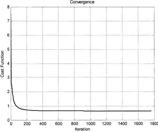
La méthode de Recuit Simulé (Simulated Annealing) est habituellement basée sur l'utilisation aléatoire de valeurs d'entrée et du calcul d'un nouveau vecteur de commande H. La fonction de coût J est ensuite comparée avec l'ancienne fonction de coût enregistrée, la plus petite des deux étant gardée. Cette méthode est très efficace pour minimiser une fonction qui possède plusieurs minimums locaux. Elle est valide à la fois pour un modèle de dynamique latérale linéaire et non-linéaire. Cependant, elle requiert un nombre élevé d'itérations à cause de son entrée aléatoire. Quelques étapes de calcul on été ajoutées afin d'améliorer la méthode de Recuit Simulé et c'est cette version améliorée qui a été utilisée pour résoudre le vecteur de commande H pour les simulations. Une étude de convergence de la méthode a été effectuée à partir de paramètres physiques d'un camion semi-remorque [ 46]. Dès les premières itérations de la méthode améliorée de Recuit Simulé, la fonction de coût diminue très rapidement pour se stabiliser après environ 200 itérations.
L'influence des différents paramètres du système conducteur/camion semi-remorque a été étudiée au chapitre 5. Désormais, les simulations peuvent être réalisées en calculant
Vll
un nouveau vecteur de commande H pour chaque cas. La perturbation pour toutes les simulations est une position initiale à y= lm et l'objectif du conducteur est de stabiliser le camion semi-remorque à y=O afin de minimiser le déplacement latéral. Pour fins de comparaison entre les différents paramètres, la première simulation sera considérée comme la référence avec les paramètres suivants:
• Le véhicule roule à 100 km/h
• Le temps de réponse du conducteur est de 0.2 secondes
Le critère d'évaluation de sécurité du camiOn semt-remorque sera la réponse en déplacement du système conducteur/véhicule en boucle fermée.
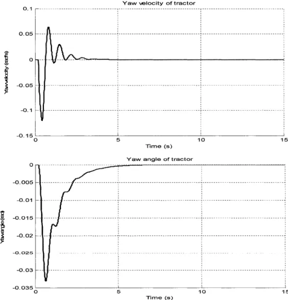
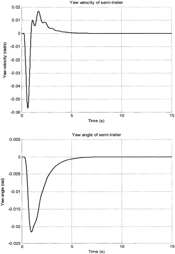
La première simulation montre une oscillation avec dépassement de l'angle de braquage des roues par le conducteur pour stabiliser le véhicule. Le déplacement latéral, quant à lui, est une très bonne réponse qui stabilise le véhicule en moins de 7 secondes, sans dépassement. La vitesse latérale du véhicule lors de la manœuvre est maximale à environ une seconde et ne dépasse pas lm/s. Les légères oscillations de la vitesse latérale du véhicule, comparativement à la position latérale, démontrent que le conducteur est plus apte à détecter la position latérale du véhicule que sa vitesse latérale. Dans le cas du tracteur et de la semi-remorque, les angles de lacet et vitesses de lacet sont bien contrôlé.
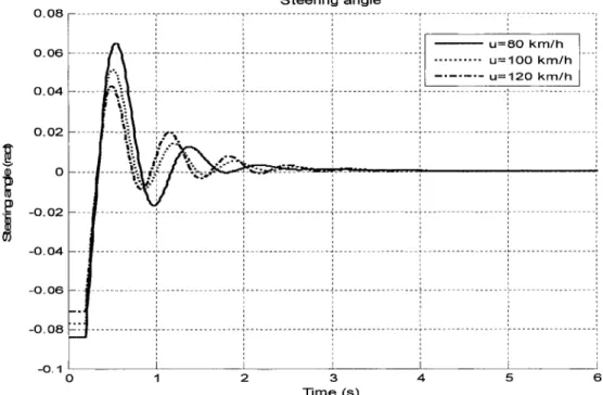
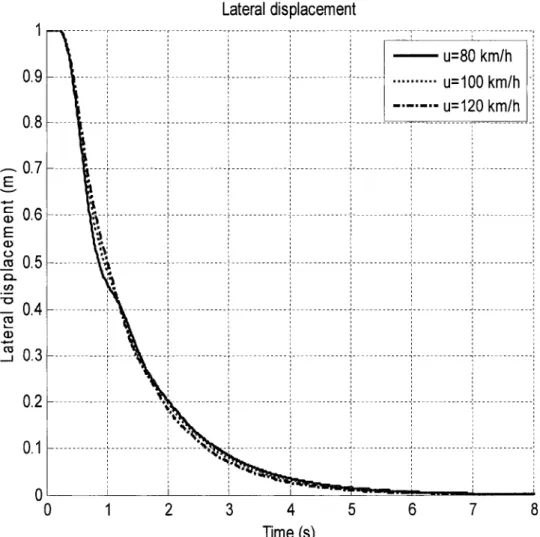
L'influence de la vitesse longitudinale du véhicule sur la stabilité du camiOn semt-remorque est maintenant étudiée. Les mêmes paramètres de véhicule et temps de réponse ont été conservés, cependant deux autres vitesses longitudinales du véhicule ont été ajoutées: 80 et 100 km/h. Les vecteurs de commande H sont calculés pour ces différentes vitesses. Pour des vitesses réduites, l'angle de braquage maximal est légèrement supérieur aux vitesses élevées. En effet, à faible vitesse, la réaction du véhicule face à un angle de braquage est moins importante qu'à haute vitesse. Pour
V111
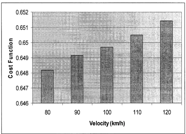
toutes les vitesses, le déplacement latéral est équivalent, alors que la vitesse latérale est légèrement plus élevée pour les faibles vitesses. On remarque les mêmes tendances pour les angles de lacet du tracteur et de la semi-remorque. Pour les vitesses de 80 à 120 km/h, par incrément de 1 0 km/h, la fonction de coût a été calculée pour chacun des cas en régime permanent. Cette étude démontre une légère augmentation de la fonction de coût presque proportionnelle avec l'augmentation de la vitesse du véhicule. Ainsi, la vitesse longitudinale a un impact sur la réponse dynamique du camion semi-remorque.
La réponse du système conducteur/camion semi-remorque est maintenant étudiée pour différentes charges de semi-remorque. La charge est variée de 5 à 25 tonnes par incrément de 5. Les résultats montrent que l'angle de braquage, la vitesse latérale et les angles de lacet pour toutes les charges sont sensiblement les mêmes. Les charges simulées de la semi-remorque n'affectent donc pas la réponse dynamique du camion sem1-remorque. Dans ces conditions, la fonction de coût a aussi été calculée pour chacun des cas en régime permanent. On remarque une légère augmentation de la fonction de coût proportionnellement avec l'augmentation de la charge.
La prochaine variable qui a été modifiée est le délai de réaction du conducteur. Originalement à .2 secondes, le délai est étudié de 0.2 à 1 seconde par intervalle de 0.1 seconde. L'angle de braquage en fonction du temps montre une importante augmentation du temps de stabilisation du véhicule, stabilisation qui n'est jamais complète pour les temps de réaction près d'une seconde. Le déplacement latéral témoigne de ces difficultés à stabiliser le véhicule pour les longs délais de réaction, cependant quoique l'angle de braquage soit en constante oscillation, le véhicule se stabilise avec peu de dépassement. Tel qu'observé précédemment, la fonction de coût augmente proportionnellement avec l'augmentation du délai de réponse du conducteur, mais d'une manière beaucoup plus importante que lors d'une augmentation de charge ou de vitesse longitudinale. Le temps de réaction du conducteur a donc un effet très prononcé sur le comportement et la stabilité du véhicule.
lX
Deux types de camwns sem1-remorque ont été comparés afin d'évaluer l'impact des différences de design sur la stabilité du système.
Le chapitre 6 présente un modèle de conducteur simplifié pour évaluer la distance de visibilité sécuritaire pour le système de camion semi-remorque/conducteur. Le modèle de conducteur simplifié est obtenu en évaluant l'importance du vecteur de commande H. Le système de commande du camion semi-remorque/conducteur a été transposé dans le domaine de Laplace. Dans le domaine de Laplace, le gain K et le délai Ta sont définis. La distance L de visibilité est présentée pour évaluer le degré de sécurité du camion semi-remorque. Les mêmes conclusions qu'au chapitre 5 peuvent être tirées concernant la sécurité. En particulier quand la distance de visibilité est réduite, par exemple en cas de mauvais temps, le conducteur doit réduire la vitesse longitudinale pour conduire le véhicule de façon sécuritaire.
Les principales contributions de cette recherche sont;
• Application de la méthode de Recuit Simulé (RS) améliorée pour étudier le système de commande du camion semi-remorque/conducteur.
• Étude de la réponse dynamique du système du camiOn semt-remorque/conducteur afin d'améliorer le comportement de conduite.
• Évaluation de l'importance des éléments de commande pour établir un modèle de conducteur simplifié et trouver la distance sécuritaire de visibilité d'un camion sem1-remorque.
La prochaine étape de ce travail serait d'analyser le système du camwn semt-remorque/conducteur dans le domaine de Laplace pour étudier la stabilité du véhicule. Les bénéfices de ces travaux futurs sont de permettre l'analyse théorique du système du camion semi-remorque/conducteur.
ACKNOWLEDGMENTS
I would like to thank my advisor, Dr. Zhaoheng Liu, for his invaluable guidance and excellent assistance during the course of this research. W orking with him has been rewarding in many ways that include and go beyond this research project.
I am deeply grateful to ali the professors who have so generously provided information and the assistance I required during my course of study and during this research project. Without their help, this work would not have been possible.
My thanks also go to the expert reviewers who took time to examine and critique the work in manuscript form.
Very special thanks go to my parents. I have been greatly influenced by them and their attitudes have always played an important role in my life.
TABLE OF CONTENTS Page SOMMAIRE ... ! ABSTRACT ... 11 RÉSUMÉ ... 111 ACKNOWLEDGMENTS ... xi
TABLE OF CONTENTS ... xii
LIST OF TABLES ... xv
LIST OF FIGURES ... xvi
NOMENCLATURE ... xviii
INTRODUCTION ... 1
CHAPTER 1 STATEMENT OF THE PROBLEM AND LITERATURE REVIEW ... 3
1.1 Statement of the problem ... 3
1.2 Literature review ... 5
1.2.1 Vehicle mo dels ... 5
1.2.2 Driver models ... 7
1.2.3 Solution method ... 8
CHAPTER 2 OBJECTIVES AND METHODOLOGY ... 10
2.1 Objectives ... 10
2.2 Methodology ... 10
2.2.1 Modeling the vehicle's lateral dynamics ... 10
2.2.2 Mode ling the human driver model.. ... 11
2.2.3 Solution method ... 12
CHAPTER 3 FORMULA TING THE VEHICLE 1 DRIVER CONTROL MODEL ... 13
3.1 The tractor semi-trailer vehicle dynamic model ... 13
3 .1.1 The trac tor in an inertial coordinate system ... 14
3 .1.2 Tractor semi-trailer dynamic system ... 16
3 .1.3 Tire forces ... 22
3 .1.3 .1 Slip angle and the cornering coefficient.. ... 22
3.1.3.2 Lateral force of the tractor semi-trailer ... 24
3 .1.4 Final equations for the vehicle' s dynamic system ... 26
3.2 Driver model with time delay ... 30
3.3 The tractor semi-trailer control system with time delay ... 31
3.4 Summary ... 32
CHAPTER 4 SOLUTION METHOD FOR SOL VING TIME-DELA YED SYSTEM AND OPTIMAL CONTROL PROBLEM ... 34
4.1 4.2 4.2.1 4.2.2 4.2.3 4.2.4 4.3 Xlll
Modified Runge-Kutta (RK) method for solving the differentiai-equation
system with time delay ... 35
The Simulated Annealing (SA) algorithm for an optimal control system36 Normal simulated annealing algorithm for a vehicle/driver dynamic system ... 37
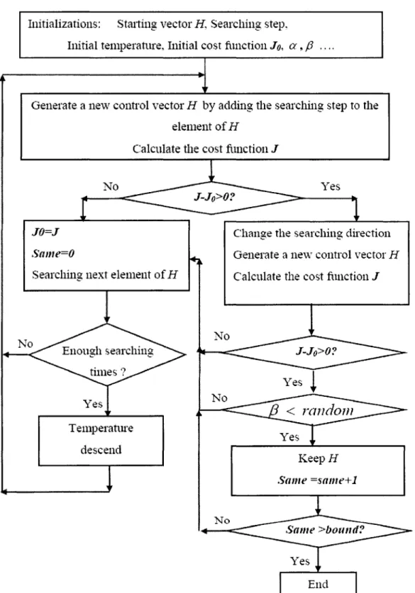
Solving the optimal control problem using improved Simulated Annealing (SA) ... 38
Parameter settings for the SA algorithm ... 41
Results of parameter setting ... 42
Summary ... 45
CHAPTER 5 SIMULATION RESUL TS ... 46
5.1 Dynamic responses of the tractor semi -trailer in cases oflateral 5.1.1 5.1.2 5.1.3 5.2 5.2.1 5.2.2 5.2.3 5.2.4 5.3 5.3.1 5.3.2 5.3.3 disturbance ... 46
Control vector H and steering angle response ... .4 7 Responses to lateral displacement and lateral velocity ... .48
Responses to yaw angle and yaw velocity ... 49
Responses to various forward speeds ... 52
Control vector H and steering angle response ... 52
Cost function at various forward speeds ... 53
Responses to lateral displacement and lateral velocity at various forward speeds ... 54
Responses to yaw angles and yaw velocities at various forward speeds. 56 Responses to various semi-trailer loads ... 59
Control vector H and steering angles at various loads ... 59
Cost function for various loads ... 60
Dynamic responses of the tractor semi-trailer at various loads on the semi -trailer ... 61
5.4 Responses to various time dela ys ... 65
5 .4.1 Control vector H and the steering angle at various time de lays ... 65
5.4.2 Cost function at various time delays ... 66
5.4.3 Lateral displacement and lateral velocity at various time delays ... 67
5.4.4 Responses to yaw angle and yaw velocity at various time delays ... 69
5.5 Comparison oftwo kinds oftractor semi-trailer. ... 72
5.5.1 Parameters for two types oftractor semi-trailer vehicle ... 72
5.5.2 Control vector H and steering angle ... 73
5.5.3 Responses to lateral displacement and lateral velocity ... 74
5.5.4 Responses to yaw angle and yaw velocity ... 76
5.6 Summary ... 80
CHAPTER 6 PREVIEW DRIVER MODEL SAFE VISIBILITY DISTANCE ... 81
6.1 Evaluating the most important elements in control vector H ... 81
6.2 The preview closed-loop control mo del ... 82
6.3 Visibility distance of the tractor semi-trailerldriver system ... 85
XlV
6.3.2 Visibility distance at various semi-trailer loads ... 86
6.3.3 Visibility distance for various time delays ... 87
6.4 Summary ... 89
CONCLUSION ... 90
LIST OF TABLES
Page
Table I Parameters for the tractor semi-trailer ... 41
Table II Optimal control vector H ... 47
Table III Control vector Hat various forward speeds ... 52
Table IV Control vector Hat various loads on the semi-trailer ... 59
Table V Control vector Hat various time delays ... 65
Table VI Parameters for the two tractor semi-trailers ... 72
Table VII Control vectors for the two vehicles ... 73
Table VIII Optimal control parameters at various forward speeds ... 86
Table IX Optimal control parameters at various loads of semi-trailer ... 87
Figure 1 Figure 2 Figure 3 Figure 4 Figure 5 Figure 6 Figure 7 Figure 8 Figure 9 LIST OF FIGURES Page
A closed-loop driver-vehicle model ... 3
Driver-parameter input model ... 4
Five-axle tractor semi-trailer [37] ... 14
Tractor yaw motion ... 15
The tractor semi-trailer ... 17
Y aw motion of the tractor semi -trailer ... 18
Bicycle model of the tractor semi-trailer. ... 18
The slip angle ... 23
A tire model ... 23
Figure 10 Tractor semi-trailer/driver control model.. ... 31
Figure 11 The annealing pro cess ... 3 7 Figure 12 Improved SA method for solving the tractor semi-trailer/driver system ... 40
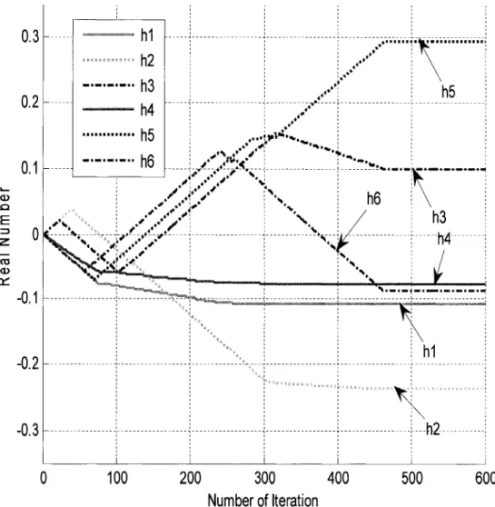
Figure 13 Variation of control vector H as a function of the number of iterations ... 4 3 Figure 14 Convergence of cost function in terms of iterations ... 44
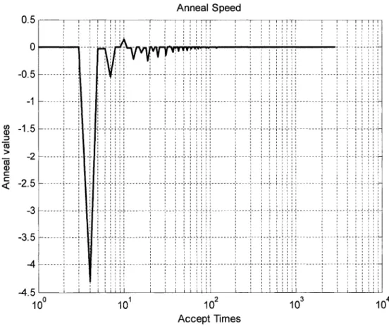
Figure 15 Anneal speed ... 45
Figure 16 Steering angle for step lateral displacement.. ... .4 7 Figure 17 Lateral displacement. ... 48
Figure 18 Lateral velocity ... 49
Figure 19 Yaw velocity and yaw angle of the tractor.. ... 50
Figure 20 Yaw velocity and yaw angle of the semi-trailer ... 51
Figure 21 Steering angle at various forward speeds ... 53
Figure 22 Cost function at various forward speeds ... 54
Figure 23 Lateral displacement at various forward speeds ... 55
Figure 24 Lateral velocity at various forward speeds ... 56
Figure 25 The tractor's yaw angle and yaw velocity at various forward speeds ... 57
Figure 26 The semi-trailer's yaw angle and yaw velocity at various forward speeds ... 58
Figure 28 Figure 29 Figure 30 Figure 31 Figure 32 Figure 33 Figure 34 Figure 35 Figure 36 Figure 37 Figure 38 Figure 39 Figure 40 Figure 41 x vu
Cost function for various loads ... 61
Lateral displacement at various loads ... 62
Lateral velocity at various loads ... 62
Yaw velocity and yaw angle of the tractor at various loads ... 63
Yaw velocity and yaw angle of the semi-trailer at various loads ... 64
Steering angle at various time dela ys ... 66
Cost function at various time dela ys ... 67
Lateral displacement at various time dela ys ... 68
Lateral velocity at various time dela ys ... 69
Y aw angle and yaw velocity of the tractor at various time delays ... 70
Yaw angle and yaw velocity of the semi-trailer at various time delays ... 71
Steering angles for the two tractor semi-trailers ... 74
Response to lateral displacement ... 75
Response to lateral velocity ... 76
Figure 42 The tractor' s response to yaw angle ... 77
Figure 43 The semi-trailer's response to yaw angle ... 78
Figure 44 The tractor' s response to yaw velocity ... 79
Figure 45 The semi-trailer' s response to yaw velocity ... 79
Figure 46 Cost function at various weight matrixes Qw ... 82
Figure 47 Lateral distance for a simple bicycle model.. ... 83
Body 1 Body2 o,x,~ 02X2Y2 OXY Axis OX 0 u 1 Tractor Semi-trailer NOMENCLATURE
The tractor's body-fixed coordinate system The semi-trailer's body-fixed coordinate system Global reference coordinate system
Road straight line
The tractor's steering angle
The tractor's constant forward velocity Heading angle
The tractor's heading angle The semi-trailer's heading angle The tractor's lateral deviation The semi-trailer's lateral deviation
The tractor's lateral velocity (in 01X1~)
The semi-trailer's lateral velocity (in 0 2X 2Y2 )
The tractor' s yaw velocity ( r1
=
~1
)The semi-trailer' s yaw velocity ( r2
=
~2
)Unit matrix
Principal yaw moment of inertia for the tractor's mass Principal yaw moment of inertia for the semi-trailer's mass Joint articulation point between tractor and semi-trailer
W eighting matrix
Distance between the tractor's front axle and centre ofmass Distance between the tractor's rear axle and centre ofmass
t Tr M1 NI K H A B
c
D FQyFn
al, J RK2 SADistance between the semi -trailer' s rear axle and centre of mass Distance betweenjoint point
Q
and the tractor's centre ofmass Distance betweenjoint pointQ
and the semi-trailer's centre ofmass Simulation timeTime delays
Symmetric positive definite matrix Damping matrix
Closed-loop gain Optimal control vector Mass matrix in (3.38) Damping matrix in (3.38) Stiffness matrix in (3.38)
Coefficient vector of steering angle in (3.38) Force at articulated point
Lateral force of the tractor' s front wheels Lateral force of the tractor's rear wheels Lateral force of the semi-trailer's rear wheels Tire characteristics for the tractor's front tires Tire characteristics for the tractor's rear tires Tire characteristics for the semi-trailer's rear tires Si de slip angle of the tractor' s front tires
Side slip angle of the tractor's rear tires Side slip angle of the semi-trailer's rear tires
Cost function
Second-order Runge-Kutta method Simulated annealing method
INTRODUCTION
Over the last few decades, the lateral dynamics and performance characteristics of articulated vehicle systems have been extensively studied, especially with regard to heavy-duty tractor trailer vehicles, for the following reasons: firstly, tractor semi-trailer vehicles play a significant role in transportation; secondly, there have been increasing concerns on how highway safety is affected by these heavy-duty tractor semi-trailer vehicles. This thesis explores the identification of lateral dynamics and parameters for tractor semi-trailer/driver systems under conditions of straight-line driving at a constant forward speed. The study of lateral dynamics focuses on modeling the tractor semi-trailer's lateral and yaw motions; parameter identification centers around recognizing the characteristics inherent in the human driver model. From a driver/vehicle closed-loop point of view, the human operator always tries to reduce lateral displacement caused by externat disturbances such as road irregularities or wind gusts, according to the vehicle's directional responses to the driver's delays in perception and reaction. Lateral dynamic responses are here defined as the vehicle's state vector: this consists of displacements and velocities. The inherent characteristics of human drivers are defined as parameters involving an optimal control model. The main goals of this thesis are to identify parameter vectors in an optimal control model and to study the dynamic behaviour of the vehicle system as driven by a predetermined optimal driver. Multi-body vehicle system equations are developed using Newton's second law; interaction between the vehicle and the road surface is modeled using a linear tire model for its lateral dynamics. A closed-loop system is achieved by combining the vehicle model and an optimal driver model with unknown parameter values. To identify the characteristics of these driver parameters, a numerical algorithm is used for searching optimal parameters while minimizing cost function. To illustrate the behaviour of the driver-vehicle system, simulations are performed using optimal control vectors under various steering conditions. In addition, a preview driver model is deduced from the
2
optimal driver model in order to demonstrate the importance of visibility distance for safe driving under a variety of driving conditions.
The chapters are organized as follows: Chapter 1 states the problem and reviews the literature. Chapter 2 de fines this study' s goals and the methodology used to ac hi eve them. Chapter 3 describes details on how to derive the tractor semi-trailer/driver control model. The numerical algorithms used for simulating delayed dynamic equations and an optimization method for determining optimal driver parameters are presented in Chapter 4. Chapter 5 demonstrates simulation results under various driving conditions. Chapter 6 introduces a preview driver model for evaluating safe visibility distance for the tractor semi-trailer/driver system. The Conclusion summarizes this project's main contributions and makes recommendations for further study.
CHAPTERl
STATEMENT OF THE PROBLEM AND LITERA TURE REVIEW
1.1 Statement of the problem
A tractor semi-trailer is a typical heavy articulated vehicle that plays a very important role in today's long-distance highway transportation. When a tractor semi-trailer is driven following a straight line at a constant forward speed, certain undefined lateral disturbances, such as wind gusts, may cause the tractor semi-trailer to stray from its straightforward direction. In such a case, the driver must guide his tractor semi-trailer back to its previous course as soon as possible by adjusting the steering wheel. The process of driving may be considered as a closed-loop driver-vehicle optimal control problem including the lateral dynamic vehicle model and the human driver model. Figure 1 demonstrates a closed-loop optimal control model, where the vehicle's input is the steering angle and the output is the tractor se mi -trailer' s states ( displacement, speed and acceleration).
Steering angle Tractor semi-trailer lateral State vector dynamic model
Steering angle State vector
Driver model
4
Optimal control of the tractor trailer is determined not only by various tractor semi-trailer designs and operating factors, but also by the driver' s interactions with the tractor semi-trailer. These interactions reveal how the driver's behaviour and the responses of the tractor semi-trailer affect one another. An excellent driver can adapt to a tractor semi-trailer and improve his performance rapidly. The behaviour of an excellent driver may be characterized as a set of inherent parameters. Thus, Figure 1 's closed-loop driver-vehicle optimal control model can be expressed by a driver-parameter input model, as shown in Figure 2.
Steering Inherent parameters
- - - . . ®
angleState vector
~ Tractor semi-trailer lateral
dynamic model
Figure 2 Driver-parameter input model
In this research project, focus has been placed on identifying lateral dynamics and parameters for a tractor semi-trailer/driver system. As shown in Figure 2, this problem does not fall under the classical framework of linear quadratic optimal control theory, because the input parameters are unknown and require identification. The Simulated Annealing algorithm is employed to search input parameters while minimizing cost function. This is achieved via large-scale searching without using a gradient method. The adopted algorithm is also well suited to both linear and nonlinear vehicle lateral dynamic models.
5
1.2 Literature review
In recent years, extensive research has been conducted in areas such as creating vehicle dynamic models [1-6]; driver models [7-15]; tire-road interaction models [16-19]; power steering models [20, 21]; automatic control models [22-32] and parameter estimations [33-35]. In this section of the thesis, we describe vehicle models, driver models and the solution method.
1.2.1 Vehicle models
The "bicycle model" is a well-known dynamic model for simulating vehicle kinetics [3 8]. In this model, a vehicle with four wheels and two axles is mode led as a one-track vehicle with two wheels (front and rear) with double lateral stiffness. J. P. Wideberg [1] has presented a simplified method for evaluating the lateral behaviour of a heavy vehicle using the bicycle model. Wideberg's results show that during simulations, dynamic effects worsen when flexible vehicle frames are taken into account.
Der Ho Wu et al. [4] have proposed a three-degree-of-freedom vehicle model, using the following assumptions:
• Nonlinearities in the springs; the dampers' behaviours are not taken into account;
• The comering force produced by a given tire is a linear function of the slip angle;
• The influence of wheel camber on lateral force generation and aligning moment are not taken into account;
• The tractor's forward speed remains constant.
In addition, in [4] the system is considered to be stable if it retums to a state of equilibrium within a finite time following a disturbance.
6
Chien Chen et al. [3] have proposed a complex vehicle model for the tractor semi-trailer. In their project, the results of the open loop experiment following a field test are compared with the results of simulating the complex vehicle model. The results of this comparison yield a linear model as follows:
M/j(t) + N/J(t) + E(q(t), q(t)) + Lq(t)
=
8 (1.4)Two properties are observed in this linear model:
• M1 is a symmetric positive definite matrix containing the vehicle system's
inertial information. 8 is the steering angle. L is a matrix.
• The N1 matrix can be interpreted as a damping matrix. Each element of the E
matrix contains tire-cornering stiffness. If the cornering stiffness is small, the vehicle system will become lightly damped and more oscillatory. For example, if the vehicle is operated on an icy road, its stability will decrease.
In work done by M.Tai et al. [2], a heavy vehicle is considered as a system of interconnected rigid-bodies interacting with the environment. In their simple model, only planar translational motion, the tractor's yaw motion, and the semi-trailer's yaw motion are considered. This model simplifies the complex model by setting certain modes at zero. By applying Newton's second law, M. Tai et al. set up the following dynamic equations:
n 4 4
F;~;al
=
L((L~~1
)sin(B1
-s1
)+(L~~)cos(s, - &1))(1.5)
i=l J=l J=l
n 4 4
F;~;a' = L((L~~
1
)cos(e1
-e1
)-(L~;1
)sin(e1
-e1))i=l j=l J=l
7
1.2.2 Driver models
Human-driver lateral control behaviour resembles a situation where a driver repeatedly tries to minimize lateral position and/or orientation tracking errors. This effort is constrained by the driver's physicallimitations.
X. Yang et al. [7] have proposed a single-loop and a multi-loop driver directional control model in order to study driver/vehicle interaction. During the directional control process, the driver acts as both sensor and controller. The driver's feedback information may in elude the tractor unit' s path and orientation errors as well as both units' lateral accelerations, yaw rates, roll angles and roll rates. These variables may be detected by the driver directly and indirectly while formulating his directional control strategy.
In [7], the considerations and assumptions associated with studying a driver's directional control behaviour include the following:
• The previewed path is expressed by a low-order polynomial function, since it includes primarily low-frequency components;
• The vehicle's path is previewed with respect to the body fixed co-ordinate system of the le ad or trailing unit;
• The driver's control actions are always directed towards minimizing the cost function.
A. Y. Ungoren et al. [8] have proposed an adaptive lateral-preview human-driver model. Their driver model is developed using the adaptive predictive control (APC) framework. The following key features characterize this APC framework:
• Use ofpreview information; • Internai model identification;
8
In this model, the driver uses predicted vehicle information in a future window to determine optimal steering action. A tunable matrix is defined in order to assign relative importance to lateral displacement, lateral velocity, yaw angle and yaw velocity in the cost function to be optimized. In this paper [8], a weighting matrix Qw is introduced in order to evaluate relative importance.
According to
T.
Legouis et al. [36], the mathematical models for driver steering control have progressed along three dimensions:• Quasi-linear; where the human operator is represented by a function with a frequency-dependent gain and phase;
• Predictive, leading to a better physical interpretation. It is assumed that the driver focuses on a fictitious point ahead in the vehicle's direction and reacts only to the vehicle's apparent lateral displacement;
• Optimal control, generated by a linear feedback loop resulting from the cascade combination of a Kalman filter and a minimum mean squared predictor.
In studying a closed-loop system for a passenger car [36], the steering model is written as
(1.6) where the constants h1, h2 , h3 and h4 are real numbers determined experimentally from
the vehicle's characteristics, speeds, and the disturbances. rjJ is heading angle. r is yaw velocity. y is lateral displacement.
1.2.3 Solution method
T. Legouis et al. [36] have proposed an optimal-approach method with time delay in order to solve the problem of driver-vehicle control. This problem does not fall under the
9
classical framework of linear quadratic optimal control theory, even without time delay. To solve this problem, the authors have devised an alternative numerical method. They begin by considering cost function to be a function of the control vector. The cost function's gradient is then expressed by the state vector and its derivative. To solve the state vector's derivative, an adjoint state equation is defined. After integrating the adjoint state equation in reverse order, from the simulation's end to its beginning, it becomes possible to evaluate the gradient. The cost function's minimum value is determined in the direction opposite to this gradient by means of a one-dimensional optimization algorithm yielding a new control vector. This algorithm must integrate the state equations, adjoint state equations, and the introduction of a one-dimensional optimization algorithm. It is limited by simulation time and step size.
M. Heinkenschloss et al. [39] have proposed an interface between the application problem and the proposed nonlinear optimization algorithm in order to solve the numerical solution of distributed optimal control problems. By using this interface, numerical optimization algorithms can be designed to take advantage of inherent problem features: for instance, splitting variables into states, controls, and scaling inherited from functional scalar products.
S. Nahar et al. [40] used the Simulated Annealing method to solve the problem of combinatorial optimization. Later, P. P. Mutalik et al. [41] proposed a parallel Simulated Annealing method for solving a similar problem involving combinatorial optimization.
P. Siarry et al. [42] have proposed a new global optimization algorithm for functions containing many continuous variables. Their new global optimization algorithm, derived from the basic Simulated Annealing method, can deal with high-dimensionality minimization problems that are often difficult to solve by all known minimization methods, with or without gradients.
CHAPTER2
OBJECTIVES AND METHODOLOGY
2.1 Objectives
The general objectives are to identify the model parameters inherent in an optimal human driver and to study the behaviour of a tractor semi-trailer vehicle system for a typical lateral regulation task following an externat disturbance during high-speed driving. The specifie objectives are:
1. Characterizing the model parameters inherent in an optimal human driver;
2. Simulating the articulated vehicle's dynamic responses using the predetermined optimal driver model;
3. Simulating the articulated vehicle's dynamic behaviour at various vehicle speeds, vehicle loads and human-driver reaction delays using optimal-driver model parameters;
4. Evaluating the effect of visibility distance on the vehicle's dynamic response using a simplified driver model.
2.2 Methodology
To achieve these objectives, research is divided into several steps; various modeling and solution methods were adopted for each step.
2.2.1 Modeling the vehicle's lateral dynamics
Using the bicycle model ([38] and [1]), the tractor semi-trailer is studied as a "two-rigid-body bicycle mode l'' consisting of the bicycle mo del and its "trailer mode l'' connected at
11
point
Q
(the fifth wheel). The lateral dynarnics of both the tractor unit and the serni-trailer unit are studied together, using a two-rigid-body bicycle rnodel, since both units have the sarne lateral velocity at point Q. Newton's second law is used to arrive at the articulated vehicle's lateral dynarnic equations, as used in [2], using the linear tire force along with sorne assurnptions such as those found in [4]. The variables used for the articulated vehicle's lateral dynarnic equations are the tractor's lateral displacernent and the yaw angles for both the tractor and serni-trailer units. The driver's steering angle is unknown.2.2.2 Modeling the human driver model
Modeling the hurnan driver involved extending to the 3-DOF rnathernatical driver-steering rnodel used by T. Legouis et al. [36], which is a 2-DOF driver-steering-angle rnodel (2.1 ).
(2.1)
The articulated vehicle/driver model (2.1), possessing single-loop [7] and lateral-preview [8] aspects, is here defined as the function of the vehicle's state vector q(t),
control vector H and tirne delay Tr. To suit the 3-DOF tractor serni-trailer dynarnic equations, equation (2.1) has been extended as follows:
S(t)
=
h1j;1 (t- Tr) + h2r1 (t- Tr) + h3r2 (t- Tr) + h4y1 (t- Tr) + h5rp
1 (t- Tr) + h6rp
2 (t- Tr)(2.2) where Yi is lateral displacement of the tractor, Yi is lateral vdocity of the tractor, epi is the tractor's yaw angle and ri =~
1
is the tractor's yaw velocity,rp
2 is the semi-trailer's yaw angle and r2=~2
is the serni-trailer's yaw velocity12
2.2.3 Solution method
The closed-loop tractor semi-trailer system has been set up using a vehicle lateral dynamic model and a driver steering model. The lateral dynamic equations include the vehicle's state vector with time delay and control vector H, as yet unidentified. Improvements are made to the Runge-Kutta method [45] in order to solve the problem of time delay in the dynamic equations. To identify control vector H, the cost function proposed by T. Legouis et al. [36] is introduced, consisting of the state vector and the weight matrix. In general, the weight matrix is considered to be equivalent to the unit matrix. Although the value of the initial state vector is known, cost function J cannot be calculated, because the state vector is known to be a function of control vector H and the previous state vector. This problem does not fall under classical control theory. The gradient method by T. Legouis et al. [36] proposed for solving this problem is limited by the linear equation. P. Siarry et al. [42] recommend the introduction of a modified Simulated Annealing algorithm to solve such problems in this type of research. Using a form of the Simulated Annealing algorithm enhanced by utilizing a fixed-search step size, we are able to seek the optimal control vector by minimizing cost function J.
CHAPTER3
FORMULA TING THE VEHICLE 1 DRIVER CONTROL MODEL
In this chapter we propose a tractor semi-trailer lateral dynamic model and a driver model. For our purposes, the tractor semi-trailer's input is the steering angle, whereas the tractor semi-trailer model's output is the state vector. As for the input of the driver model, this is the state vector a human driver can detect following a certain time delay; the output of the human driver model is the steering angle. In this way, a closed-loop tractor semi-trailer/driver control system with time delay can be created.
3.1 The tractor semi-trailer vehicle dynamic model
An articulated vehicle such as a tractor semi-trailer consists of the tractor unit and a semi-trailer unit. These are assumed to be rigid bodies with fixed centre of gravity. A five-axle tractor semi-trailer is the type of heavy articulated vehicle used in this thesis. We chose a tractor unit with a single driving axle and rear twin-axle, linked by a wheel coupling to a twin-axle trailer unit. Figure 3 shows a typical five-axle tractor semi-trailer running on a highway.
In order to study the vehicle's dynamics, we used a coordinate system; this was attached to the vehicle in order to describe the vehicle's motion. The tractor semi-trailer's motion was described within an x-y inertial reference frame. The extended bicycle model for automobiles was used to analyze the tractor trailer's motion. The tractor semi-trailer vehicle was considered to be moving along a straight line at a constant forward speed with a small angular deviation in heading. The suspension and brakes were ignored. Following Newton's second law and after applying sorne simplifications, it was then possible to set up a three-degree-of-freedom (3-DOF) tractor semi-trailer vehicle dynamic model.
14
Figure 3 Five-axle tractor semi-trailer [37]
3.1.1 The tractor in an inertial coordinate system
The first analysis we performed concerned the motion of the tractor that can be described within an x-y inertial reference frame. Figure 4 shows a view of the tractor as seen from above. The coordinates
x
and y locate the centre of mass of the tractor with respect to the ground; rjJ is the angle between the centerline of the tractor and a line on the ground parallel to the x-axis. The x-y axes are presumed to be neither accelerating nor rotating. The parameters of the tractor are a 1 and b 1 or the distance from the centreof mass to the front and rear axles respectively; m1 is the mass, and/z1 is the moment of
15
y
0
x
Figure 4 Tractor yaw motion
Normal motion is considered to have a constant speed
u
along the x-axis; the variables needed to describe the lateral motion are therefore primarily y(t) and r/J(t). Althoughx(t) is also required, generally speaking, under conditions of normal and disturbed
motion, it is here assumed that
x ::::::
u is a constant; therefore, x(t) =ut+ constant. Thus speed, u, plays the role of a parameter in the analysis. In normal motion, because there is no lateral disturbance, y ,y ,
rjJ and ~ all vanish, and the rigid body proceeds along the x-direction at a constant speed u.When motion is disturbed,
y
is assumed to be small as compared to the constant speedu; values rjJ and ~ are also small. The speed, brjJ is therefore small compared to the constant speed u . This means that the small angle approximations cos rjJ :::::: 1 and sin rjJ :::::: rjJ may be used wh en taking disturbed motion into account. The kinematic equations can therefore be written as
drjJ - = r dt dy= v +ur/J dt 16 (3.1) (3.2)
where y is the lateral displacement, rjJ is the yaw angle, r is the yaw velocity, v is the lateral speed, and u is the constant forward speed.
The side forces are determined to be F1 and F,. Of course, vertical forces at both axles are necessary in order to support the weight of the body; however, these forces play no role in the body's lateral dynamics. Three equations of motion can be written easily, because the tractor is described in an inertial coordinate system and is undertaking a plane motion. The force equations are arrived at by multiplying mass by acceleration in two directions; the moment is found to be equal to the rate of changing of angular momentum around the z-axis. The angle rjJ is assumed to be very small for the disturbed motion; the equations for the disturbed motion are
mit= 0 m(v+ur)
=
F1 +F,(3.3) (3.4) (3.5)
where u is the constant forward speed of the vehicle, m is the total mass of the vehicle, v
is its lateral speed, and r is its yaw velocity.
3.1.2 Tractor semi-trailer dynamic system
The second analysis takes into account the motion of both the tractor and the semi-trailer, connected at point Q. These are also described within an x-y inertial reference frame. Figures 5 and 6 show a view of the tractor semi-trailer. The global coordinates x and y located at the centres of mass of the tractor and semi-trailer ( rjJ1 and rjJ2 respectively) are
17
the angles between the centreline of the tractor semi-trailer and aline on the ground that is parallel to the x-axis. The x-y axes are presumed to be neither accelerating nor rotating.
z
c2
c1
1•
1 u0
b2
b1
i 1a1
x
~'"~~.~~·-~---~ Figure 5 The tractor semi-trailerThe parameters of the tractor are a1 and bi ; the distance from the centre of mass to the
front and rear axles, c1 (or the distance between joint point Q and the centre of mass);
mi is the mass, and I zi , the moment of inertia surrounding the centre of mass with respect to the vertical axis. The parameters for the semi-tractor are b2 , the distance from the centre of mass to the rear axles;
c
2 , the distance between joint point Q and the masscentre; m2, the mass, and I zz , the moment of inertia surrounding the centre of mass with respect to the vertical axis. The distance between the two tires, which are fixed on the same si de of the axle, is not taken into account. Lateral forces for both tires are taken to be twice that for a single tire.
18
y
v2 2fr2 2fr2 y0
x
Figure 6 Yaw motion of the tractor semi-trailer
When sorne approximations are applied with respect to the tractor semi-trailer, such as disregarding the distance between the tractor's two rear axles, this yields a bicycle model of the tractor semi-trailer, as shown in Figure 7.
y
c
x
19
According to the tractor dynamics analyzed in subsection 3 .1.1, two kinematic equations can be arrived at for the tractor when motion is disturbed:
dfA
- = r dt 1
(3.6)
(3.7)
According to the tractor dynamics analyzed in subsection 3 .1.1, two kinematic equations can also be written for the semi-trailer in the event of disturbed motion:
(3.8)
(3.9)
For the tractor, the side forces are 2F11 and 8Fr1 for the front wheel and the rear wheel,
respective! y. F Qy is the side force generated by the semi-trailer. The above analysis shows that equations of motion for the tractor unit can be expressed as follows:
(3.10) (3 .11)
For the semi-trailer, the side forces are 8Fr2 for the rear wheel. FQy is the side force generated by the tractor. The analysis above shows that equations of motion for the semi-trailer unit can be expressed as follows:
20
(3.13)
The tractor's lateral velocity at joint articulation point Q can be represented as:
(3.14)
The semi-trailer's lateral velocity at joint articulation point Q can be represented as:
(3.15)
Because the tractor and semi-trailer are connected at joint articulation point Q, they have the same lateral velocity at this point:
Thus, the lateral velocity of the semi-trailer at point
Q
can be written as:Based on the derivative in (3.17), the lateral acceleration of the semi-trailer can be written as:
Based on equation (3.12) and equation (3.18), the force, FQycan be written as:
(3.16)
(3.17)
(3.18)
21
The resulting · dynamic equations for the tractor semi-trailer system are obtained by displacing force F Qy by equation (3 .19). Equation (3 .1 0) can then be written as:
After simplification, the above equation is expressed by the state vector and the tire forces.
(3.20)
Equation (3.11) can be written as:
After simplification, the above equation is expressed by the state vector and the tire forces.
(3.21)
Equation (3.13) can be written as:
After simplification, the above equation is expressed by the state vector and the tire forces.
22
The equations of motion (3.20),(3.21),(3.22) corresponding to 3 DOF consist of the dynamic equations presented in terms of lateral tire force.
3.1.3 Tire forces
Accurate nonlinear mathematical models of tire-road interaction, verified by experiment, have been developed for use in computer simulations of vehicle dynamics [38]. These models are useful for simulating complex vehicle models that are in turn utilized for predicting the response of proposed vehicle designs. Generally, simple linear models of tire force generation are used to analyze vehicle dynarnics under the influence of small disturbances away from a basic state of motion. Slip angle and the comering coefficients are used to describe tire-road interaction.
3.1.3.1 Slip angle and the cornering coefficient
Because the wheel supports the load, a normal force exists between the road' s surface and the tire' s contact patch. If a small lateral force is then applied to the wheel, a corresponding lateral force will arise in the contact patch between the tire and the road surface due to friction. Although the lateral force may be too small to cause the tire to slide sideways over the surface, the wheel will no longer continue to move in the direction in which it has been pointed. Rather, it will acquire a sideways or lateral velocity in addition to its forward velocity. Thus, the total velocity vector of the wheel will point in a different direction than the direction of the wheel' s centre plane. This angle between the wheel and the direction in which the wheel moves when a lateral force is applied is called the slip angle, a . [ 4 3] An example of a slip angle is shown in Figure 8.
23
u
. y a~-U F 1'.
1 .Figure 8 The slip angle
When analyzing the stability of vehicles using pneumatic tires, it is common to use a linear model showing the relationship between the lateral force generated by the tire, F,
and the slip angle, a .
F
Skid
a
24
Figure 9 shows that over a certain range, lateral force and the slip angle are found to be nearly proportional to each other. The linear tire force model will apply in an approximate way for small values of the lateral force and for small values of the slip angle. As long as the lateral force remains small enough so that the tire does not begin to skid, the slip angle remains quite small. For small slip angles, a proportionality constant, the cornering coefficient Ca , can be defined as the slope of the line that relates lateral force to slip angle. This means that the lateral force can be expressed as:
(3.23)
At large slip angles, the tire begins to skid and the force-vs-slip-angle relationship becomes significantly nonlinear. At a certain slip angle, the lateral force reaches a maximum.
3.1.3.2 Lateral force of the tractor semi-trailer
When a disturbance is slight, the linear tire model is used to analyze the tire force generated by the tractor semi-trailer. The tractor's front-tire force can be expressed as:
where
8 is the front steering angle.
Front-tire force is then expressed using lateral velocity, yaw velocity, constant forward speed, vehicle parameters and steering angle.
25
F _ -C (v' +a1r1 _ s:)
f i - fi u
u
(3.24)
The tractor's rear-tire force can be expressed as
where
Rear-tire force is then expressed using lateral velocity, yaw velocity, constant forward speed and vehicle parameters.
(3.25)
The semi-trailer's rear tire force can be expressed as
where
The semi-trailer's rear-tire force is expressed using lateral velocity, yaw velocity, constant forward speed, and vehicle parameters.
26
(3.26)
3.1.4 Final equations for the vehicle's dynamic system
From equations (3.24), (3.25) and (3.26), tire forces for the tractor semi-trailer can be expressed in terms of vehicle parameters, state variables and tire-comering coefficients. Substituting the tire force into the tractor semi-trailer dynamic equations yields the equations for the tractor semi-trailer's dynamic system.
(m1 + m2)v1 + (m1 + m 2 )ur1 - m 2c1
J\-
m 2c 2r
2=
-2C/I(VI +airi -S)-8Cri(vi-biri)-8Cr2(v2u u
- c 1 m 2
v
1 - c 1 m 2 ur 1 + (! z 1 + c 12 m 2 )1\
+ c 1 c 2 m 2r
2=
(3.27)
- 2a]C fi (v, + a,r, - 8) + 8b!C ri (VI -bir!)+ 8c!C r2 ( v2 - b2r2) (3.28)
u u u
In equations (3.27), (3.28) and (3.29), there are four variables: v1 , v2 ,r1 ,r2 ; however, a 3-DOF dynamic model has only three independent equations. Using equation (3.11), v2 is eliminated and the equations become:
(3.30)
( 1 2 ) • c 1 m 2 v 1 - c 1 m 2 ur 1 + z 1 + c 1 m 2 r 1 + c 2 c I m 2 r 2 v 1 + a 1 ri r 1 ( v 1 - b 1 ri )
=
-2a 1C n(----'---~=--- 5)+
8b 1C u u u and - c 2 m 2 v 1 - c 2 m 2 ur 1 + c 1 c 2 m 21\
+ ( 1 z 2 + ci
m 2 )r
2=
8 ( b 2 + c 2 ) C r 2 ( u ( rjJ 1 - rjJ 2 ) + v 1 - cI ri - c 2 r 2 - b 2 r 2 ) uFollowing calculation and simplification:
2a1C f i - 8b1C r i - 8c1C ,2 + (( m 1 + m 2 ) u + ) r1 u 8C,2(b2 +c2 ) A. CA. C s: - r2 + 8Cr2'f'I- 8 r2'f'2
=
2 Jiu u and • 2 • . 2a1C11 -8b1Cri -8c1C,2- clm2vi + (JzJ +ci m2)rJ + clc2m2r2 + ( )vi
u
2a]2C fi+ 8bl2C ri+
s<c
r2 Sel (b2 + c2 )C r2+ ( - c1m 2u)r1 + r 2
u
u
- 8c1C ,2r/J1 + 8c1C ,2r/J2=
2a1C 115 and • • ( / 2 ) " 8(b2 +c2)C,2 - c 2 m 2 v 1 + c 1 c 2 m 2 ri + z 2 + c 2 m 2 r 2 - v 1 u (8c1(b 2 +c2)C,2 ) 8(b2 +c2 ) 2 C, 2 + - c 2 m 2 u r1 + r 2 u u - 8(b2 + c2)C r2rP1 + 8(b2 + c2)C r2rP2=
0From equation (3.2), the relative equation of
y
1 and v1 is obtained:27
(3.31) (3.32) (3.33) (3.34) (3.35)28
(3.36)
After differentiation, the relative equation of
y
1 and1\
is obtained:(3.37)
Lastly, the tractor semi-trailer's dynamic equations, which are expressed by the state vector, can be written as follows:
lA,
Al2A,r,J lB"
Bl2 A2I A22 A 23 ~~ + B 21 Bn A31 A32 A 33 r2 B 31 B 32le"
cl2
c,
r· J
lD"]
+c
21c
22c
23 <Pl=
D2I 8c
31c
32c
33 <P 2 D3I where8 Steering angle of the tractor
</J
1 = Heading angle of the tractor
<jJ
2 Heading angle ofthe semi-trailer
y1 Lateral deviation of the tractor
r1 Y aw velocity of the tractor ( r1
=
~1
) r2 Y aw velocity of the semi-trailer ( r2=
~2
)Ali =ml +m2 A12
![Figure 3 Five-axle tractor semi-trailer [37]](https://thumb-eu.123doks.com/thumbv2/123doknet/7487047.224135/34.915.167.733.185.624/figure-five-axle-tractor-semi-trailer.webp)