Are Private Equity Funds of Funds managed by more risk-tolerant Private Equity Firms necessarily more risky?

(1)

HEC Paris

Strategy and Business Policy Prof. Oliver Gottschalg, PhD

Are Private Equity Funds of Funds managed by more

risk-tolerant Private Equity Firms necessarily more risky?

A thesis submitted in partial satisfaction of the requirements for the degree

Master of Science in Management (Grande ´Ecole)

by

Torben Rabe

Torben Rabe Brookweg 88a

21465 Wentorf bei Hamburg Germany

(2)

To my parents, Sabine and Lars,

for their endless love and support. My sincere gratitude to Prof. Gottschalg, PhD,

(3)

ABSTRACT OF THE MASTER THESIS

by

Torben Rabe

Master of Science in Management (Grande ´

Ecole)

HEC Paris, 2016

Professor Oliver Gottschalg, PhD

Are Private Equity Funds of Funds managed by more

risk-tolerant Private Equity Firms necessarily more risky?

The aim of this thesis is to analyze the risk-return characteristics of portfolios of Private Equity Funds, so-called Funds of Funds (FoFs). I used a large data set of 5,539 Euro-pean, U.S. and Asian funds with historic performance information from Preqin covering vintage years from 1977 to 2011. The dataset includes 1,312 buyout funds and 774 ven-ture capital funds.

This thesis shows that the risk and return characteristics of FoFs are significantly influ-enced by portfolio construction parameters related to the number of fund investments, the length of the investment period, the investment rhythm, the vintage year, the size focus, the geography and the selection ability of the investor.

To this aim, I present a framework to analyze the risk profile of FoFs using fund per-formance data. Through Monte Carlo simulations, I am able to test how the portfolio construction and fund selection decisions at the Fund of Funds (FoF) level affect the risk- return properties of the portfolio.

This framework allows me to derive a probability distribution of historically possible FoF performances, and conclude on the risk profile of a FoF. The risk associated to a FoF investment is significantly smaller than the one for a fund investment. The risk-mitigating effect of diversification depends, however, on the portfolio’s investment period length, investment rhythm, size focus, geography, selection ability and fund type. I find that the weight allocation technique has only a negligible effect on the risk of FoFs.

(4)

List of Figures

1 An exemplary portfolio containing loss-making deals . . . 16

2 Illustration of Skewness using a Beta Distribution . . . 17

3 Kernel density of portfolio TVPI for overall dataset . . . 24

4 Kernel density of portfolio TVPI for buyout funds . . . 24

5 Analysis of TVPI dispersion by dataset . . . 25

6 Utility vs. Number of Funds (dataset) . . . 26

7 Risk-return ratio vs. Number of Funds (dataset) . . . 26

8 Analysis of TVPI dispersion by Investment Period . . . 29

9 Utility vs. Number of Funds (Investment Period) . . . 30

10 Risk-return ratio vs. Number of Funds (Investment Period) . . . 30

11 Analysis of TVPI dispersion with different Investment Rhythm . . . 34

12 Skewness of portfolio TVPI vs. Number of Funds . . . 35

13 Excess kurtosis of portfolio TVPI vs. Number of Funds . . . 35

14 Utility vs. Number of Funds . . . 36

15 Risk-return ratio vs. Number of Funds . . . 36

16 Boxplot of TVPI dispersion by Size Focus . . . 40

17 Analysis of TVPI dispersion by Size Focus . . . 41

18 Utility by Size Focus . . . 42

19 Analysis of TVPI dispersion by Weight Allocation . . . 46

20 Utility vs. Number of Funds . . . 47

21 Boxplot of TVPI dispersion by Region Focus . . . 50

22 Analysis of TVPI dispersion by Region Focus . . . 51

23 Utility vs. Number of Funds (Region Focus) . . . 52

24 Risk-return ratio vs. Number of Funds (Region Focus) . . . 52

25 Boxplot of TVPI dispersion by Selection Ability . . . 56

26 Analysis of TVPI dispersion by Selection Ability . . . 57

27 Utility vs. Number of Funds (Selection Ability) . . . 58

28 Risk-return ratio vs. Number of Funds (Selection Ability) . . . 58

29 Boxplot of TVPI dispersion by Fund Type . . . 63

30 Analysis of TVPI dispersion by Fund Type . . . 64

(7)

32 Risk-return ratio vs. Number of Funds (Fund Type) . . . 65

33 Boxplot of TVPI dispersion by dataset . . . XII 34 Skewness-to-risk Ratio vs. Number of Funds (dataset) . . . XIII 35 Boxplot of TVPI dispersion by Investment Period . . . XIV 36 Skewness-to-risk Ratio vs. Number of Funds (Investment Period) . . . . XV 37 Skewness-to-risk ratio vs. Number of Funds (Investment rhythm) . . . . XVI 38 Skewness-to-risk Ratio vs. Number of Funds (Size Focus) . . . XVII 39 Boxplot of TVPI dispersion by Weight Allocation . . . XVIII 40 Skewness-to-risk Ratio vs. Number of Funds (Weight Allocation) . . . . XIX 41 Skewness-to-risk Ratio vs. Number of Funds (Region Focus) . . . XX 42 Skewness-to-risk Ratio vs. Number of Funds (Selection Ability) . . . XXI 43 Skewness-to-risk Ratio vs. Number of Funds (Fund Type) . . . XXII

List of Tables

1 Overview of overall dataset by selection ability . . . 7

2 Overview of overall dataset by region focus . . . 7

3 Overview of overall dataset by fund size category . . . 7

4 Results of overall dataset - TVPI . . . 22

5 Results of overall dataset - Other measures . . . 22

6 Buyout funds - TVPI . . . 23

7 Buyout funds - other measures . . . 23

8 Investment Period: Results of buyout funds - TVPI . . . 28

9 Investment Period: Results of buyout funds - Other measures . . . 28

10 Results of one- and two-sided MWW test, CI=95% (PERACS Risk Coef-ficient vs. Investment Period) . . . 28

11 Equal Rhythm: Results of buyout funds - TVPI . . . 31

12 Equal Rhythm: Results of buyout funds - Other measures . . . 31

13 Random Rhythm: Results of buyout funds - TVPI . . . 32

14 Random Rhythm: Results of buyout funds - Other measures . . . 32

15 Results of one- and two-sided MWW test, CI=95% (PERACS Risk Coef-ficient vs. Investment Rhythm) . . . 32

(8)

17 Small and medium buyout funds (Smid) - other measures . . . 38

18 Large buyout funds - TVPI . . . 38

19 Large buyout funds - other measures . . . 38

20 Results of one- and two-sided MWW test, CI=95% (PERACS Risk Coef-ficient vs. Size Focus, only large cap and smid focus) . . . 39

21 Random weights: buyout funds - TVPI . . . 44

22 Random weights: buyout funds - other measures . . . 44

23 Equal weights: buyout funds - TVPI . . . 44

24 Equal weights: buyout funds - other measures . . . 44

25 Pro rata weights: buyout funds - TVPI . . . 45

26 Pro rata weights: buyout funds - other measures . . . 45

27 Results of two-sided MWW test, CI=95% (PERACS Risk Coefficient vs. Weight Allocation) . . . 45

28 American buyout funds - TVPI . . . 49

29 American buyout funds - other measures . . . 49

30 European buyout funds - TVPI . . . 49

31 European buyout funds - other measures . . . 49

32 Result of one- and two-sided MWW test, CI=95% (PERACS Risk Coef-ficient vs. Region Focus) . . . 50

33 Upper median buyout funds - TVPI . . . 55

34 Upper median buyout funds - other measures . . . 55

35 Lower median buyout funds - TVPI . . . 55

36 Lower median buyout funds - other measures . . . 55

37 Results of one- and two-sided MWW test, CI=95% (PERACS Risk Coef-ficient vs. Selection Ability) . . . 56

38 Buyout funds - TVPI . . . 61

39 Buyout funds - other measures . . . 61

40 VC funds - TVPI . . . 61

41 VC funds - other measures . . . 61

42 Real Estate funds - TVPI . . . 62

43 Real Estate funds - other measures . . . 62

44 Early Stage funds - TVPI . . . 62

(9)

46 Result of one- and two-sided MWW test, CI=95% (PERACS Risk Coef-ficient vs. Fund Type) . . . 63

(10)

Glossary

CAPM Capital Asset Pricing Model. 13 e.g. exempli gratia. 7

FoF Fund of Funds. III, 1, 4, 5, 10, 11, 13, 21, 27, 31

FoFs Funds of Funds. III, 1, 2, 4, 5, 8, 10, 20, 21, 27, 37, 48, 53, 59 i.e. id est. 4, 10, 15, 17, 53

ILPA International Limited Partner Association. 12, 13 IPO Initial Public Offering. 48

MPT Modern Portfolio Theory. 3, 4

MWW Mann-Whitney-Wilcoxon. 19, 27, 33, 43, 48, 53, 59 pdf probability density function. 18

PE Private Equity. 1

TVPI Total Value to Paid In. 19, 21, 27, 33 USA United States of America. 7, 9

(11)

1 Introduction

”The word ’risk’ derives from the early Italian risicare, which means ’to dare’. In this sense, risk is a choice rather than a fate. The actions we dare to take, which depend on how free we are to make choices, are what the story of risk is all about. And that story helps define what it means to be a human being.”

Peter L. Bernstein, Against the Gods: The Remarkable Story of Risk

Private Equity (PE) provides equity capital to private companies. Due to its attractive risk-return characteristics and especially its supposedly1 _{low correlation with other}

as-set classes, Private Equity has become more and more popular among institutional and sophisticated investors. David Swensen, the longtime investment chief at the Yale Uni-versity Endowment Fund, has pioneered a model that favors a longer investment horizon and committing capital to illiquid investments such as Private Equity. This approach has yielded superior returns in the past (Swensen (2009)). Other sophisticated investors have followed suit. However, Private Equity is still widely perceived as a risky asset class, and many investors struggle with the strategic capital allocation to this asset class (Gottschalg et al. (2015)).

The emergence of Private Equity FoFs coincides with this development. A FoF allocates capital from investors in multiple underlying funds on their behalf. FoF investors are typically pension funds, banks, insurance companies, corporate investors, and other FoFs (Weidig et al. (2005)). Private equity FoFs are now contributing more than 10% of the total capital in private equity, i.e. venture capital and buyout funds (Preqin (2014)). However, their risk profile is not well understood due to their intransparent and illiquid nature, as well as the limited access to performance figures.

The majority (59%) of investors interviewed by Preqin stated that the main reason they used FoF investments was to diversify their portfolios. This seems intuitive at first glance: Investors commit to private equity FoF to gain access to a wide range of underlying fund types, investment strategies, underlying assets, fund managers, vintage years2_{, industries, geographies and currencies. (Preqin (2014)). A FoF should have}

reduced risk in comparison to a single fund investment due to the non-perfect correlation between funds and a second level diversification effect, as FoFs consist of funds which themselves consist of investments. A greater diversification level has two important implications. First, a wider range of fund managers and their applied strategy is included

1_{Phalippou and Zollo (2005) show that, in reality, the performance of private equity funds is}

pro-cyclical as it positively co-varies with both the business cycles and public stock-markets. 2

(12)

in the portfolio, which usually has a positive effect. More importantly, a greater degree of diversification at the fund level implies a greater degree of diversification in terms of portfolio companies. A portfolio of 10 private equity funds containing 80 to 150 underlying portfolio companies has different risk characteristics than a portfolio of, say, 100 funds with 800 to 1,500 companies, which have been acquired at different stages of the business cycle. Thus, FoF investors should have clear diversification benefits. FoFs need to understand their own risk profile, if they are to convince potential investors of their lower risk.

The aim of this thesis is to clarify the diversification benefits and how portfolio construc-tion decisions such as the number of underlying funds, the geographic focus, selecconstruc-tion ability, fund size focus, investment period and investment rhythm affect the risk-return characteristics of portfolios.

Therefore, I simulated historical FoFs and performed a thorough analysis of their risk-return characteristics under different scenarios. Historical FoFs are constructed by creat-ing portfolios of historical Funds that are randomly selected from the Preqin dataset given some varying constraints described in 4.1 and while respecting the time line. Through Monte Carlo simulation techniques, I am able to analyze how different portfolio design decisions impact the risk-return characteristics of the portfolio.

The remainder of this paper is structured as follows. After this introductory section, I discuss the importance of diversification in the context of Private Equity as an asset class. After that, I will present the data used for this research along with its limitations and possible biases. I then describe the used framework & model before I go over to the results for each hypothesis. Finally, I will conclude the paper with a short summary of the main findings.

(13)

2 Diversification

”You’re missing the big picture”, he told her. ”A good album should be more than the sum of its parts.”

Ian Rankin, Exit Music

2.1 Private Equity and Modern Portfolio Theory

According to Modern Portfolio Theory (MPT), the more diversified a portfolio and the more uncorrelated its components, the less idiosyncratic risk3 contributes to the risk of the overall portfolio. The notion of diversification is best summarized by Benoit Mandel-brot, who recommended ”broad, very broad diversification with small equal allocations” Taleb (2012). Diversification is a fundamental part of the investment approach of almost all institutional and sophisticated investors. Including diversification in the investment approach is supported by a wide range of academic research since its establishment by Markowitz (1952).

However, one needs to be careful to apply MPT to Private Equity because of the unique nature of Private Equity as an asset class and challenges related to data availability and other modeling assumptions. MPT assumes that investors pay no taxes or transaction fees and can optimize their portfolios through a mean-variance optimization. Models based on MPT may be adequate for the universe of publicly traded instruments but rely on parameters that are instable, unreliable or even unavailable in Private Equity. Most investors assume that Private Equity investments have a low correlation with the public market, which makes the asset class look attractive in the eyes of portfolio managers. Nevertheless, MPT does not offer the right tools to analyze Private Equity returns and to construct Private Equity portfolios for the following reasons (see Meyer (2014)):

• The market for Private Equity is not efficient: valuations are usually unreliable and infrequent and the investments are illiquid because of long holding periods and few buyers and sellers. Investors usually only get access to the company’s financial data once they invest in the private company. This makes it difficult, if not impossible, to measure risk as the volatility of a time series. The interpretation of correlation as a measure of dependence can be misleading.

(14)

• Due to the illiquidity of Private Equity investments and the long investment period of between 10 to 12 years, the assumption of MPT that all investors have the same time horizon is not true.

• As shown in section 3.1.1, private Equity fund returns are highly non-normal, which goes against the MPT assumption of normally distributed returns.

If we go one step above to the FoF level, the properties look a little different. Mathonet and Weidig (2004) show that for a diversified portfolio of funds the return multiple distribution of FoFs is nearly normally distributed with flattening tails, id est (i.e.) the return multiple distribution function of FoFs approaches the normal distribution function as we add more and more funds to the portfolio and increase the diversification level. Thus, while investors should not use MPT on the fund level, the notions of this theory may be applicable to the FoF level. Consequently, I will MPT-related concepts such as standard deviation or the risk-return ratio, which is similar to the sharpe ratio, but will also focus on the PERACS Risk CurveTM _{and PERACS Risk Coefficient}TM _{as the}

measure of risk.

2.2 The Impact of Diversification on the Portfolio

The overall goal of portfolio construction is to select and combine assets with funda-mentally different attributes to optimize the risk-return characteristics of the portfolio and to ultimately meet the manager’s objectives. Diversification is a technique used to protect the portfolio against the impact of adverse events and unfavorable outcomes. However, with an increasing number of assets the portfolio’s return reverses to the aver-age market performance. As Warren Buffett states, wide diversification is only required when investors do not understand what they are doing. Investors may use the principle of concentration to achieve growth instead (Meyer (2014)).

Thus, before discussing whether an ’optimal’ level of diversification exists, the benefits and limits of diversification techniques need to elaborated on.

2.2.1 The Benefits of Diversification

Diversification, at least to a certain degree, has an undeniably positive effect on the risk-return characteristics of a portfolio. There are very few investors that would invest only in one asset on the Fund or FoF level, given that investors have sufficient capital. The benefits are (Meyer (2014)):

(15)

• Diversification reduces the contribution of idiosyncratic risk to the risk of the over-all portfolio. Private Equity funds have on average in 20-25 investments in their portfolio. Private Equity FoFs in turn also have on average 20-30 funds in their portfolio. Thus, investors gain exposure to hundreds of Private Equity investments by investing in Private Equity FoFs. The FoFs managers improve the portfolio’s risk-return properties by including more funds in their portfolio and gaining expo-sure to different industries, geographies, fund types or vintage years.

• Diversification may make the fund raising process for FoF managers easier. With an increasing diversification level there is an increasing stability and predictability of portfolio behavior and notably more reliable cash flows. Thus, it may be easier to find investors.

• For the same reasons diversification may enable higher leveraging to manage a portfolio’s risk profile.

These benefits are mutually exclusive, but not necessarily collectively exhaustive.

2.2.2 The Limits to Diversification

The level of diversification might have an upper limit, however, when one considers the impact of diversification under risk-return aspects. Not only will diversification increase the investor’s protection against the downside, but it also has a detrimental impact on the portfolio‘s upside.

• If one accepts the idea that only the best funds provide a competitive return, diver-sification will eventually prove counterproductive and lead to a mean reversion of the portfolio’s return. At some point there will be a lack of high quality investment opportunities and the overall performance of the portfolio will be reduced if less attractive investments are included to increase the level of diversification, if the investor has an asset selection ability higher than the average selection ability.4

• Overdiversification is costly and leads to high transaction costs, due diligence and monitoring costs and administrative costs that reduce the overall portfolio’s return.

4_{If the investor has a lower selection ability, diversification might prove to be a more powerful tool.}

(16)

2.3 The ”Optimal” Level of Diversification

Considering the benefits and limits to diversification, the question emerges which level of diversification is ’optimal’ for FoFs. Answering this question is not trivial and has been subject to academic research (see especially Gottschalg et al. (2015), but also Ljungqvist and Richardson (2003), Korteweg and Sorensen (2010),Cornelius (2011) or Hochberg et al. (2007). Mathonet and Weidig (2004) found that the maximum diversification ben-efit is achieved with just twenty to thirty underlying funds. Gottschalg et al. (2015) shows that the benefits of diversification also depend on the size focus and the selection ability of the FoF. The question of how much to diversify on the Fund of Fund level depends, among other things, on the investor’s risk appetite, selection skills and the returns targeted for the overall portfolio. FoF managers who are convinced of their se-lection abilities to identify attractive investment opportunities may find it more effective to use concentrated portfolios that include only the most attractive investment opportu-nities according to their assessment. Thus, the optimal level of diversification ultimately depends on the risk appetite of investors.

The question will be revisited in section 5.

2.4 How to achieve Diversification

There are three ways to construct a diversified portfolio (Meyer (2014)):

1. The top-down approach is based on a construction of the overall portfolio, de-termining allocation ranges first and then searching for investments that fit these allocations. Using this approach, portfolio managers prioritize the choice of sec-tors, countries, trends and vintage years as opposed to the selection of individual assets. The major drawback of this approach is that in reality it is not always possible to stick to the allocations the strategy proposes.

2. Using the bottom-up approach, portfolio managers take the opposite direction and focus on screening all investment opportunities based on their individual attrac-tiveness and risk-return characteristics. Portfolio considerations such as geographic diversification are assumed to only have a subordinate role.

3. The naive approach includes a portfolio construction technique where the portfolio components have an equal portfolio weights. Portfolios that are constructed in such a way are found to be not significantly inferior to the other approaches. However, investing the same amount of capital in every fund in the portfolio introduces a

(17)

bias as it is implicitly a bet that smaller funds will perform better than the larger ones.

3 Data

3.1 Data sample and Descriptive Statistics

On the fund level, the Preqin dataset comprises 5,539 funds with historic performance information from Europe, United States of America (USA) and Asia provided by Pre-qin covering vintage years from 1977 to 2011. Funds after 2011 are not included in the dataset because younger funds may not be fully liquidated yet and their performance multiple given by Preqin may still be subject to valuation principles applied to unrealized investments. The data set includes 1,312 buyout funds and 774 venture capital funds. The other types of funds are summarized in the appendix.

Table 1 gives an overview of the descriptive statistics of the overall dataset including different fund types. For most of my thesis, i used buyout funds.

Table 1: Overview of overall dataset by selection ability

Selection Ability Number of Funds Mean TVPI Median TVPI Minimum TVPI Skewness Kurtosis 1 Lower median 2606 1.14 1.19 0.00 0.36 6.37 2 Upper median 2933 2.19 1.78 0.68 10.42 167.25

Table 2: Overview of overall dataset by region focus

Region Focus Number of Funds Mean TVPI Median TVPI Minimum TVPI Skewness Kurtosis

1 Asia 407 1.62 1.40 0.30 4.79 34.72

2 Europe 1236 1.56 1.42 0.00 4.66 48.99

3 US 3896 1.75 1.51 0.00 11.55 212.42

Table 3: Overview of overall dataset by fund size category

Fund Size Category Number of Funds Mean TVPI Median TVPI Minimum TVPI Skewness Kurtosis

1 Large 992 1.47 1.43 0.12 1.68 11.03

2 Medium 3123 1.65 1.46 0.00 13.21 287.42 3 Small 1424 1.94 1.56 0.01 8.36 120.64

(18)

3.1.1 Statistical Tests on Funds for Simulation

Test of normality. The Kolmogorov-Smirnov test checks for the normality of the fund performances.5 _{With a probability of 0.00%, the performances of buyout funds are}

normally distributed.6 _{Therefore standard concepts of financial theory, which assume}

normally distributed returns, are not applicable for the modeling of Private Equity port-folios on the fund level. This includes standard deviation, correlation and any other ratios that use these measures, exempli gratia (e.g.) Sharpe ratio or the Sortino ra-tio. As the fund performance is not normally distributed, non-parametric tests like the Mann-Whitney test and the Kruskal-Wallis test have to be used (Meyer (2014)).

However, we will assume that the returns of portfolios on the Fund of Fund level are nor-mally distributed. The Kolmogorov-Smirnov test statistic indicates that the distribution of portfolios with a higher diversification level is close to a normal distribution. As shown later, this assumption is also supported by the change in skewness and kurtosis towards a normal distribution when comparing Fund level and Fund of Fund level returns. Using the Mann-Whitney test statistic, significant differences between Venture Capital (VC) and buyout funds are found as a whole. Therefore the simulation and analysis of FoFs is done solely for buyout funds first. I will look at the risk-mitigating effect of diversification for VC and other fund types in section 5.8.

3.2 Limitations of the dataset

Although I am working with a relatively large data set of 5,539 funds, I am looking at smaller subsets to isolate and investigate certain effects. For that reason, some years or regions may be over- or underrepresented, as explained in 3.3.

Furthermore, I am assuming that the TVPI and other variables of the funds in the dataset are independent and identically distributed random variables. The independence of variables is one of the central tenets of conventional asset allocation frameworks built around the concept of ”normality” of asset returns.

5_{The normal distribution is a statistical distribution commonly used to model asset class returns in}

traditional Mean-Variance Optimization frameworks.

6_{The Kolmogorov-Smirnov test is used to decide if a sample comes from a population with a specific}

(19)

3.3 Possible Biases

Before discussing the framework and results of my analysis, I have to describe potential biases in the dataset. The Preqin dataset is a combination of self-reported informa-tion provided by fund managers and US performance data published by public pension schemes. Because of the nature of this dataset, a number of potential biases could arise. First, a potential survivorship bias could occur if the funds stop reporting data once their fund returns decrease or are expected to perform poorly, as Gottschalg et al. (2015) point out. Gottschalg et al. (2015) also argue that portfolio managers follow their own specific objectives in the design of their private equity portfolios. Thus, fund selection decisions and skills of the portfolio managers could influence the data. For both of these reasons, the fund returns in the dataset are likely to be too high as compared to the actual average returns of all private equity funds.

Furthermore, the data might be impacted by a selection bias due to the self-reported nature of the data. The Preqin data was provided by fund managers. It could be the case that only high-performing funds report their performance. Weidig et al. (2005) argue that reporting funds should have no incentive to bias their performance data if the data set is based on voluntary reporting. Kaplan and Schoar (2003) suggest that a selection bias does not occur in the Venture Economics data set that they used.

The number of funds per vintage year in the Preqin data set varies. For instance, there are only 8 funds in 1982, but 522 funds in 2007 in the data set. This has implications for the Monte Carlo simulation because a low number of funds for a vintage year may lead to two different sources of error. Firstly, statistical errors and lower significance may occur. Secondly, there might be a systematic bias due to a lower coverage in a vintage year. If one vintage year is underrepresented, subsequent vintage years might also be underrepresented in the simulation. Since the maximum distance of vintage years of the funds in the simulated portfolios is constrained by the investment period, some periods, such as the 1980’s may be underrepresented. The same holds for different regions: In contrast to European (maximum number of funds: 119 in 2007) and Asian (maximum number of funds: 52 in 2008) funds, US funds show a relatively high coverage (maximum number of funds: 313 in 2007).

The majority of the funds in the dataset have the USA as their region focus (3379 US funds and 734 US buyout funds). The simulated portfolios are designed in such a way that all funds in the portfolio have the same region focus. Thus, simulated portfolios predominantly consist of US funds.

(20)

Finally, younger funds (i.e. funds with vintage years after 2011) might not be fully liquidated yet. If some funds in the dataset are not fully realized, the valuation principles by which their return is measured differ. To mitigate this effect, I excluded private equity funds raised with vintage years after 2011. It is worth noting that, while these biases may influence the average returns and overall dispersion of the data, the relationship between different variables (especially portfolio design decision variables) might not be affected.

4 Framework & Model

I simulated historical FoFs because performance data on historical FoFs is rare and standard portfolio theory cannot be applied to model FoFs risk (Weidig et al. (2005)). For that reason, a Monte Carlo simulation technique is used to compute the performance and risk of FoFs with varying characteristics. Ideally, all possible combinations of funds would be simulated. This, however, is not feasible due to the high number of possible combinations. Nevertheless, the more portfolios are constructed randomly, the closer the sample resembles the population of all possible portfolios. Given the large number of simulated portfolios, the simulation in this thesis delivers a good level of approximation.

4.1 Monte Carlo Simulation

To construct a historical fund, a hypothetical FoF is simulated in a random year, and funds are assigned given specific constraints. A first fund is randomly drawn and all other funds in the portfolio follow constraints that depend on the characteristics of the first fund drawn and the hypothesis tested. Firstly, only funds the FoF could have invested in during the chosen investment period can be included. For instance, if the first fund drawn is from 1995 (i.e. its vintage year is 1995) and the investment period is 5 years, then only funds with vintage year from 1995 to 1999 can be included in the portfolio. Secondly, only funds with the same region focus can be included. Thus I implicitly assume that FoFs only invest in one region. For example, if the first fund has a region focus on Europe, then the subsequent funds are also focused on Europe. Thirdly, only funds with the same fund size category can be included. Doing that, I implicitly assume that FoFs only invest in funds with a similar fund size category. The fund size categories are small (≤ 100mn USD), medium (≤ 800mn USD) and large (> 1,500mn USD). According to Gottschalg et al. (2015), the small, medium and large size categories reflect the commonly agreed definition of fund sizes. Additionally, small and

(21)

medium funds are summarized as ’smid’ funds (0-800mn USD) to compare against the large fund category.

To analyze the risk-mitigating effect of increasing the diversification level, I randomly create 1,000 random portfolios of Funds which consist of 1, 5, 10, 15, 20, 25, 30, 50 or 100 underlying Fund(s). For hypotheses 1, the overall dataset including different fund types is used. For hypothesis 8, four different fund types are compared (buyout, vc, early stage, real estate). For the other hypotheses, only buyout funds are used to simulate portfolios in order to isolate the risk-mitigating effect of changing certain parameters. Each Fund can be drawn several times between different portfolios, but never in the same portfolio. The performance of FoF portfolios is the average performance of the underlying funds. The return dispersion of the simulated portfolios is calculated using two different approaches. First, the difference between the maximum and minimum portfolio returns is calculated and analyzed in form of boxplot graphics.7 _{Second, I will}

apply the approach used in Gottschalg et al. (2015), more precisely the PERACS Risk CurveTM _{and Coefficient}TM _{explained in 4.3.2.}

Related to section 2.4, this thesis mimics both the top-down and naive approach to simulate portfolios according to pre-defined allocations. For the Monte Carlo simulation, I used both equal portfolio weights as well as random weights and pro rata weights.8 There are several ways to achieve diversification. FoF managers increase the number of funds, alternate the geographic focus or size focus of the funds they are invested in, or include different vintage years in the portfolio. The model used in this thesis tests how the risk-mitigating effect of increasing the number of funds in the portfolio changes under different circumstances.

7_{The whiskers of the boxplot graphics in section 5 represent the minimum and maximum, not}

quan-tiles.

(22)

4.2 Hypotheses

When running the Monte Carlo Simulation, several hypotheses were tested. The results of these tests are shown in section 5. The simulation of portfolios of funds was designed differently for each hypothesis. I did find evidence for most, but not all, hypotheses.

1. Hypothesis 1: The risk of Funds and Funds of Funds is reduced as the number of investments and funds, respectively, is increased.

(a) The diversification effect can already be seen when comparing the median & average risk-return profile of Private Equity Funds and Funds of Funds. (b) At the same time, the marginal diversification benefit of increasingly large

portfolios decreases rapidly (as can be measured by the number of investments or Funds in the portfolio). There exists a number of Funds beyond which the marginal cost exceeds the marginal benefit of diversification.

2. Hypothesis 2: There exists a risk-mitigating effect by increasing the investment period and thus diversifying the vintage years in the portfolio. However, the diver-sification effect is smaller than the diverdiver-sification effect from increasing the number of funds in the portfolio, as also shown by Mathonet and Weidig (2004).

3. Hypothesis 3: The diversification effect of increasing the number of underlying funds is influenced by the investment rhythm.

4. Hypothesis 4: Portfolios of small-cap funds enjoy a disproportionate risk-mitigating effect when the diversification level is increased (Gottschalg et al. (2015)).

5. Hypothesis 5: Increasing the number of funds has a different risk-mitigating effect when the portfolio weights within the Fund of Fund are allocated equally, randomly, or pro rata.

6. Hypothesis 6: There exists a difference in the optimal number of funds in a Private Equity portfolio depending on the regional focus of the fund.

7. Hypothesis 7: Investors with a low selection ability enjoy a higher risk-mitigating effect from increasing the number of funds in the portfolio than investors with a high selection ability.

8. Hypothesis 8: Increasing the number of funds has a different risk-mitigating effect for different fund types.

(23)

4.3 Measures

4.3.1 Performance Measures

The TVPI is a measure of gross returns to invested to capital. It is a cumulative realisation ratio and is also called multiple. According to the International Limited Partner Association (ILPA), the TVPI is the ratio of the current value of remaining investments within a fund, plus the total value of all distributions to date, relative to the total amount of capital paid into the fund to date.

T V P I = DP I + RV P I DP I = Distributionscumulative

CapitalP aidIncumulative

RV P I = ResidualV alue CapitalP aidIncumulative

The TVPI is commonly used in the context of Private Equity investments and funds according to the ILPA. The used Net TVPI is net of fees, expenses and carry.9

There are several reason why this thesis does not focus on the IRR as the primary per-formance measure. As Gottschalg points out, the IRR method puts too much emphasis to the returns generated early in the life of a PE fund. Morevover, IRR tries to express the annual performance of a PE fund for the time from the inception of this fund to its last cash flow, while the money is in fact invested gradually (and returned gradually) in Private Equity. Hence the IRR formula makes implicit assumptions about the returns generated while the money is not yet (or no longer) invested by the PE fund and these assumptions distort the performance assessment. Furthermore, the calculation of the pooled IRR10 _{would significantly complicate the analysis of the simulated model. In the}

TVPI multiple calculation, the reinvestment rate is assumed to be zero. In the IRR calculation, it is assumed that capital can be reinvested at the same rate. Harris, Jenk-inson, and Kaplan (2011) report weighted average TVPIs of 1.76-2.30 for buyout funds and 2.19-2.46 for VC funds.

9_{Carry = carried interest, i.e. percentage of profits that general partners receive out of the profits}

of the investments made by the fund.

(24)

4.3.2 PERACS Risk CurveTM and PERACS Risk CoefficientTM

Because of the illiquid nature of Private Equity investments, it is difficult to determine the volatility of underlying portfolio companies or funds, and even more difficult to calculate the volatility of the overall Fund or FoF. Other analyses of Private Equity related to the Capital Asset Pricing Model (CAPM) model tend to be complex to conduct and difficult to interpret (Driessen et al. (2012)). Instead, the PERACS Risk CurveTM and PERACS Risk CoefficientTM developed by Oliver Gottschalg and Peracs are part of a profit-distributions method that measures the risk within a private equity portfolio. The risk profile for a Private Equity Fund or FoF is created through plotting the cumulative profits. First, the contribution of each individual investment to the total profit of the portfolio is calculated. The contribution can be either calculated in terms of simple dollars or any other currency or in terms of net present value (NPV)) of each investment in a private portfolio. Then, the investments are ranked according to their contribution.

Based on this, we can plot a graphical representation of the cumulative function of the empirical distribution of profits. The resulting PERACS Risk CurveTMis a performance-distribution curve constructed by plotting the percentage of a fund’s investments, ordered by their profit contribution, on the x-axis and the percentage of profit contribution from the corresponding fund on the y-axis. Every point on the Curve corresponds to a performance statistic. Consequently, one can for example see that the worst x% of the portfolio contribute to y% of the portfolio’s profit. The PERACS Risk CurveTM _is

equivalent to the Lorenz Curve11 _{used in economics.}

11_{Max Lorenz developed the lorenz curve in 1905, which represents the inequality of wealth}

(25)

The PERACS Risk CurveTM is defined as: Fi = i/n Si = i X j=1 Yj Li = Si/Sn where:

• n refers to the number of investments.

• yi is a sequence of i = 1 to n For n investments, with a sequence of yi, i = 1 to n

that is indexed in increasing order (yi ≤ yi+1).

• The PERACS Risk CurveTM _{is the resulting continuous linear function from}

con-necting (Fi, Li).

The PERACS Risk CurveTM _{is equal to the ’line of perfect equality’ (i.e. the curve}

would be a 45◦straight line) if every investment generates the same absolute profit. The ’case of perfect inequality’ describes the case when a single investment generates all the portfolio profits (Gottschalg et al. (2015)).

Using this approach, investors can easily assess a portfolio’s risk characteristics and compare them with the portfolio’s return. Overall, the more curved the graph is, the more profits are concentrated in a low number of investments. As Gottschalg et al. (2015) points out, Private equity investors may differ in their preferences for different shapes of the PERACS Risk CurveTM_.

Another concept created by Gottschalg and Peracs is the PERACS Risk CoefficientTM_.

It refers to the area between the ’line of perfect equality’ and the PERACS Risk CurveTM_.

The higher the coefficient, the more unequal the profit distribution (i.e. 0 = perfectly distributed profit, 1 = perfectly concentrated profit). The Coefficient is equivalent to the Gini Coefficient12. The PERACS Risk CoefficientTMis calculated through a method similar to a method developed and used by Chen et al. (1982), who calculate the Gini coefficient for economies with individuals of negative net wealth. The PERACS Risk CurveTM_{, as well as the PERACS Risk Coefficient}TM_{, are designed to be independent}

of the absolute amount of profits generated by the portfolio (Gottschalg et al. (2015)). Gottschalg argues that this makes it possible to compare risk profiles of different Private Equity portfolios, independent of their absolute returns.

(26)

Figure 1: An exemplary portfolio containing loss-making deals

Source: Peracs and Chen et al. (1982)

The PERACS Risk CoefficientTM _{can be intuitively understood using the areas in}

fig-ure 1:

P ERACS Risk Coef f icientTM= A + B A + B + C

As Chen et al. (1982) point out, the area (A + B) can be considered as the area of concentration whereas area C is an area of equalization. In a portfolio without loss-making deals, B + C = 0.5 and P ERACS Risk Coef f icientTM _{= B/2, which is identical}

(27)

4.3.3 Skewness and Kurtosis

Skewness is a parameter that measures the asymmetry in a random variable’s proba-bility distribution. The probaproba-bility density functions of exemplary beta distributions in figure 2 differ only in their skewness. The mean and the standard deviation are iden-tical. The graph on the left is positively skewed. The graph on the right is negatively skewed. The skewness for symmetric distributions, such as the normal distribution or in the middle figure, is zero (Meyer (2014)). Investors generally prefer a positive value for the skewness of returns so that the right tail is longer and more positive extreme returns can be achieved.

(a) Positive skewness (b) Zero skewness (c) Negative skewness

Figure 2: Illustration of Skewness using a Beta Distribution

The skewness of a distribution is calculated as:

skewness = n P i=1 (xi−¯x)3 n σ3

Kurtosis is a measure of whether the data is more peaked or flat compared to a normal distribution. A higher kurtosis indicates that more of the variance is due to infrequent extreme deviations. Normal distributions have a kurtosis of three. Distributions with a kurtosis value greater than three (so-called leptokurtosis) are characterized by a high peak and fat tails. Distributions with a kurtosis lower than three (so-called platykur-tosis) are characterized by a less peaked distribution and thinner tails. High kurtosis is associated with having ’fat tails’, i.e. the payoff of winners and the losses associated with losers tend to be more extreme. Thus, investors who are convinced of their selection ability may prefer a high kurtosis (Meyer (2014)). A risk-averse investor, on the other hand, prefers a distribution with low kurtosis so that returns tend to be not far away from the mean.

(28)

The kurtosis of a distribution is calculated as: kurtosis = n P i=1 (xi−¯x)4 n σ4

4.4 Other Measures

Shortfall risk is the probability that the portfolio of funds will not achieve a set target multiple:

P (T V P IP) ≤ T V P IP,T

where T V P IP is the net return multiple of the portfolio P and T V P IP,T is the target

multiple for the portfolio.

Mathonet and Weidig (2004) introduced an expected utility function in their analysis of mean variance-skewness-kurtosis-efficient portfolios. Similary, this thesis analyzes the realized utility of simulated portfolios. The realized utility is a probability density function (pdf), which has four moments: mean, variance, skewness and kurtosis. If the four moments are not realized but expected values, the investor’s utility can be expressed with a Taylor series.

In this thesis only realized values are analyzed with the following function: Up = A ∗ T V P Ip− 1 2 ∗ B ∗ variancep+ 1 3!∗ C ∗ skewnessp− 1 4!∗ D ∗ kurtosisp where:

• Up is the utility of a portfolio investor.

• T V P Ip is the average return multiple of the portfolio, which is desirable. The

return coefficient A hence has a positive sign and is set to 4 in this thesis.

• B is the risk aversion coefficient of the average investor assumed in this thesis. The risk aversion coefficient is set to 4 in this thesis. The variance of the T V P Ip is

undesirable, hence the negative sign.

• Positive skewness is desirable, negative skewness is undesirable, hence the positive sign. The skewness coefficient C is set to 2 in this thesis.

• Excess kurtosis above 3 indicates a more peaked distribution, with fatter tails than normal. Generally, kurtosis is undesirable, which would imply a negative

(29)

sign. However, in the context of diversifying Private Equity risk, the question whether kurtosis is beneficial or not is not so clear. For instance, for an investor with high selection ability, a fat tail would be more desirable. This is why the kurtosis aversion coefficient D is set to zero in this thesis.

The standard deviation of the portfolios’ return multiple is a risk indicator for the return dispersion for a given investment strategy. In this context, the standard deviation is defined as: σp = s Pn i=1(T V P Ii− T V P I) n

where σp is the standard deviation of the given investment strategy, TVPI is the final

return of the portf olioi and n is the number of simulated portfolios for the given number

of funds, investment period etc.

Other measures are the to-risk ratio and the risk-return ratio. The skewness-to-risk ratio tries to capture the trade-off between skewness (which is utility-enhancing for investors) and risk.

Skewness − to − risk = Skewness σi

The risk-return ratio is similar, but not equal, to the sharpe ratio. It captures the trade-off between the reduced average return multiple and the reduced risk from diver-sification. Risk-return

SR = ((T V P Ii− 1) σi

For comparing different distributions, I used a Mann-Whitney-Wilcoxon (MWW) test. The MWW is a nonparametric test of the null hypothesis that independent two samples come from the same population. The MWW test can also be used to determine whether the one population tends to have larger values than the other. In that sense, the MWW test is similar to a t-test. Unlike the t-test, however, the MWW does not require the assumption of normal distributions. MWW has a power advantage when one of the samples is drawn from a skewed, a peaked distribution or a mutimodal dis-tribution De Winter and Dodou (2010). I used the MWW in particular to compare the PERACS Risk CoefficientTM _{of simulated portfolios under different circumstances.}

For example, when I compared US and European buyout funds, the MWW test indi-cated which of the two samples of simulated portfolios had the higher PERACS Risk CoefficientTM _value.

(30)

4.5 Limitations of the Model

The Total Value to Paid In (TVPI) return multiple does not incorporate the time value of money nor the opportunity costs of capital.

As expected, the average returns remain relatively stable when comparing Funds and FoFs, and kurtosis and skewness all decrease. However, my simulations do not account for the diseconomies of scale and program size, which would normally decrease returns. The coefficients in the utility function are set arbitrarily. They do not account for different risk-return preferences of individual investors or types of investors. Rather, an average investor with a high preference for a high average return is assumed.

(31)

5 Results

5.1 Hypothesis 1: Overall dataset and diversification level

Hypothesis 1a: The risk of Funds and Funds of Funds is reduced as the number of investments and funds, respectively, is increased. The diversification effect can already be seen when comparing the median & average risk-return profile of Private Equity Funds and Funds of Funds.

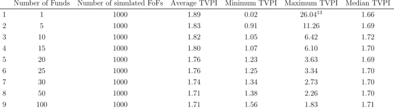
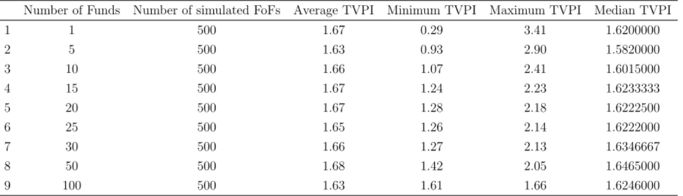
Table 4 shows the TVPI of simulated FoFs with different number of funds in the portfolio and an investment period of five years. I used the overall dataset, equal portfolio weights and a random investment rhythm to simulate the portfolios. Comparing the return multiples of Funds (n = 1) and simulated FoFs (n > 1), it can be seen that the average TVPI is relatively similar for Funds or FoFs, although it is worth mentioning that the mean TVPI is reduced as n is increased. While both the minimum and maximum TVPI revert to the mean as n is increased, the median TVPI is higher for any value for n other than 1.

This is because the FoF distribution is less skewed with more funds in the portfolio, as can be seen in 5. The Kernel distributions in figure 3 and figure 4 show that with an increasing number of funds, the TVPI multiple of the portfolio is more concentrated around the mean. The mean and median come closer, implying a more symmetric distribution.

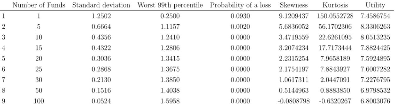
Figure 5 shows that the standard deviation of FoF returns is reduced as n is increased. Similarly, the worst 99th percentile of the 1000 simulated portfolios in terms of perfor-mance already averages a TVPI above 1 with 10 underlying funds, and the probability of a loss is reduced to 0.0000% with 15 underlying funds (Table 5).

Hypothesis 1b: At the same time, the marginal diversification benefit of increasingly large portfolios decreases rapidly (as can be measured by the number of investments or Funds in the portfolio). There exists a number of Funds beyond which the marginal cost exceeds the marginal benefit of diversification.

The utility of the hypothetical average investor can be seen in figure 6. For both the overall dataset as well as the combined data of buyout and venture capital funds, the utility sharply increases as n is increased. It can be seen that the distribution of FoF returns has much thinner tails and is less skewed than the distribution of individual fund returns. Interestingly, the skewness and kurtosis of the overall dataset become negative for n = 100.

(32)

However, the utility then levels off around 20 to 30 funds in the portfolio. For both datasets, the utility reaches a maximum at n = 25. This is mainly due to the variance reduction, as the variance coefficient in the utility function is set to 4. Figure 5 shows the reduction in skewness, which is unfavorable for the investor, but is outweighted by the reduction in variance at first, as can be seen in figure 6. The skewness coefficient in the utility function is set to 2. Thus, the utility is increased as n is increased. However, as n is increased, the return multiple is reduced, thus decreasing the utility for n > 30. As n is increased, the marginal diversification benefit of increasingly large portfolios (measured by the number of investments or Funds in the portfolio) decreases rapidly: not only will the investor incur additional costs, but the investor will aslo give up some chances to reap some extraordinary returns. Therefore, the utility function shows a plateau at n = 25 given the assumed utility function and the used dataset.

To sum up, there exists a trade-off between a lower risk level through diversification and diminishing returns paired with reduced marginal benefits of diversifiaction. As Borel (2004) states, ”LPs have recognized that beyond a certain point, the return of any addi-tional diversification is likely to diminish [...] To avoid such a regression though excess diversification to an undesired mean, a growing number of investors are aggressively cutting back on the number of managers they want to commit the money to.”

Table 4: Results of overall dataset - TVPI

Number of Funds Number of simulated FoFs Average TVPI Minimum TVPI Maximum TVPI Median TVPI

1 1 1000 1.89 0.02 26.04 1.66 2 5 1000 1.83 0.91 11.26 1.69 3 10 1000 1.82 1.05 6.42 1.72 4 15 1000 1.80 1.07 6.10 1.70 5 20 1000 1.76 1.23 3.63 1.69 6 25 1000 1.76 1.25 3.34 1.70 7 30 1000 1.74 1.34 2.73 1.70 8 50 1000 1.71 1.38 2.26 1.70 9 100 1000 1.71 1.56 1.83 1.71

Table 5: Results of overall dataset - Other measures

Number of Funds Standard deviation Worst 99th percentile Probability of a loss Skewness Kurtosis Utility

1 1 1.2502 0.2500 0.0930 9.1209437 150.0552728 7.4586754 2 5 0.6664 1.1157 0.0020 5.6836052 56.1702306 8.3306263 3 10 0.4356 1.2410 0.0000 3.4719559 22.6261095 8.0513235 4 15 0.4322 1.2806 0.0000 3.2074234 17.7173444 7.8824425 5 20 0.3036 1.3415 0.0000 2.2315254 7.9658189 7.5924895 6 25 0.2868 1.3675 0.0000 2.1754197 7.8843927 7.6007282 7 30 0.2130 1.3850 0.0000 1.0617311 2.0447091 7.2276795 8 50 0.1516 1.4038 0.0000 0.5144963 0.8883850 6.9798532 9 100 0.0524 1.5958 0.0000 -0.0808798 -0.6320267 6.8003076

(33)

Table 6: Buyout funds - TVPI

1 1 1000 1.89 0.02 26.0413 _1.66 2 5 1000 1.83 0.91 11.26 1.69 3 10 1000 1.82 1.05 6.42 1.72 4 15 1000 1.80 1.07 6.10 1.70 5 20 1000 1.76 1.23 3.63 1.69 6 25 1000 1.76 1.25 3.34 1.70 7 30 1000 1.74 1.34 2.73 1.70 8 50 1000 1.71 1.38 2.26 1.70 9 100 1000 1.71 1.56 1.83 1.71

Table 7: Buyout funds - other measures

1 1 1.2502 0.2500 0.0930 9.1209437 150.0552728 7.4586754 2 5 0.6664 1.1157 0.0020 5.6836052 56.1702306 8.3306263 3 10 0.4356 1.2410 0.0000 3.4719559 22.6261095 8.0513235 4 15 0.4322 1.2806 0.0000 3.2074234 17.7173444 7.8824425 5 20 0.3036 1.3415 0.0000 2.2315254 7.9658189 7.5924895 6 25 0.2868 1.3675 0.0000 2.1754197 7.8843927 7.6007282 7 30 0.2130 1.3850 0.0000 1.0617311 2.0447091 7.2276795 8 50 0.1516 1.4038 0.0000 0.5144963 0.8883850 6.9798532 9 100 0.0524 1.5958 0.0000 -0.0808798 -0.6320267 6.8003076

(34)

0 1 2 3 4 5 6 0.0 0.5 1.0 1.5 2.0 TVPI Density

Overall dataset TVPI Distribution

1 fund 5 funds 10 funds 15 funds 20 funds 25 funds 30 funds 50 funds 100 funds

Figure 3: Kernel density of portfolio TVPI for overall dataset

0 1 2 3 4 5 0 1 2 3 4 TVPI Density

Buyout funds TVPI Distribution

1 fund 5 funds 10 funds 15 funds 20 funds 25 funds 30 funds 50 funds 100 funds

(35)

0.0 0.5 1.0 1.5 2.0 Standard deviation Number of Funds Standard de viation 0.0 0.5 1.0 1.5 2.0 Number of Funds 1 10 20 30 50 100 Dataset Overall dataset Buyout funds 0 1 2 3 4 5 6 0.0 0.2 0.4 0.6 0.8 1.0 CDF by Selection Ability TVPI Fn(x) Dataset Overall dataset Buyout funds 0 2 4 6 8 10 12 Skewness Number of Funds Sk e wness 0 2 4 6 8 10 12 1 10 20 30 50 100 Dataset Overall dataset Buyout funds 0 50 100 150 200 Kurtosis Number of Funds K ur tosis 0 50 100 150 200 1 10 20 30 50 100 Dataset Overall dataset Buyout funds

(36)

5 6 7 8 9 Number of Funds Utility 5 6 7 8 9 1 5 10 15 20 25 30 50 100 Dataset Overall dataset Buyout funds

Figure 6: Utility vs. Number of Funds (dataset)

0 5 10 Number of Funds Risk−retur n r atio 0 5 10 1 5 10 15 20 25 30 50 100 Dataset Overall dataset Buyout funds

(37)

5.2 Hypothesis 2: Investment period

Hypothesis 2: There exists a risk-mitigating effect by increasing the investment period and thus diversifying the vintage years in the portfolio. However, the diversification effect is smaller than the diversification effect from increasing the number of funds in the portfolio, as also shown by Mathonet and Weidig (2004).

In standard Private Equity FoFs, the total capital available gets invested mostly during the investment period, i.e. the first three to five years of the funds lifetime, but also afterwards, in a more targeted manner, to follow on the most successful investments (Weidig et al. (2005)). The distributions of capital to limited partners are done as soon as investments get exited, mostly during the divestment period, i.e. the remaining funds lifetime. Therefore, Private Equity fund investments should be made over the full course of the economic cycle and should not be concentrated in any one year to reduce the risk of getting in or out at the wrong time. Thus, there should be a clear diversification benefit by increasing the investment period length and thus diversifying vintage years in the portfolio.14

Table 8 shows the TVPI of simulated FoFs with 25 funds in the portfolio for different in-vestment periods. I used buyout funds, equal portfolio weights and a random inin-vestment rhythm. Both the average and median TVPI increase with the length of the investment period. The minimum TVPI for investment period lenghts ≤ 2 is above 1.

The risk measures are summarized in table 9. The standard deviation of the TVPI first sharply increases from a 1-year investment period to 2 years, before it decreases from investment period lengths 4 to 6. The utility goes up as the investment period length increases, because both the skewness and the average return increase.

Figure 8 shows the evolution of different TVPI dispersion metrics for different investment period lengths. In terms of standard deviation, portfolios with shorter investment periods benefit most from adding funds to the portfolio. Portfolios with investment periods 1 and 2 have the lowest standard deviation for n ≤ 50. Both the skewness and kurtosis of the portfolios are reduced significantly for all investment periods and decrease to almost 0 for investment periods 1 & 2.

The utility by number of Funds in figure 9 shows that the diversification benefit by adding funds to the portfolio exists for all investment periods. The optimum level of diversification is different for different investment periods, but is between 10 and 30 funds. Generally, the utility increases if the investment period length is increased. However, the effect on the investor’s utility is smaller in relative and absolute terms compared to adding more funds to the portfolio.

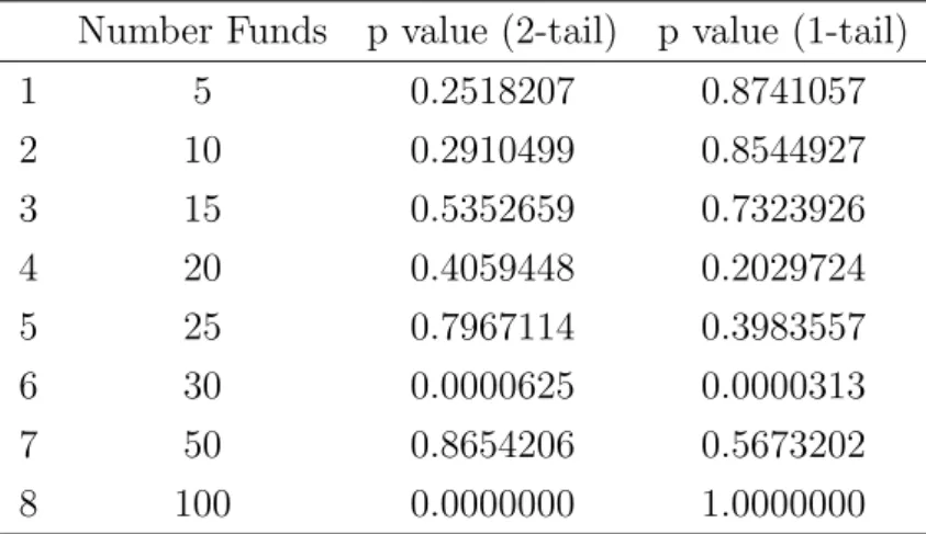
The MWW test of the PERACS Risk CoefficientsTM for portfolios with 3 and 6 years investment period length reveals no significant difference. At 0.05 significance level, I conclude that the risk coefficients for the two period lengths are identical populations for all values of n except for n = 30 (Table 10). Thus, a difference in risk cannot be observed using the risk coefficients.

14_{In this thesis the EVCAs definition of vintage year as the year of fund formation and first drawdown}

(38)

In short, I observe a diversification benefit of increasing the length of the investment period. All risk and return metrics are improved by increasing the length of the in-vestment period. This is intuitive, as the FoF investor gains more and more exposure to the economic cylce and avoids having to choose the perfect timing. In the words of Maximilian Broenner from LGT Capital Partners, ”analyzing the different fund raising and return cycles over the last 20 years makes one thing very clear: the perfect timing in an asset class which requires long-term commitment and does not offer daily liquidity is rather impossible” (taken from Mathonet and Meyer (2008)).

Table 8: Investment Period: Results of buyout funds - TVPI

Investment Period Number of simulated FoFs Average TVPI Minimum TVPI Maximum TVPI Median TVPI

1 1 1000 1.72 1.34 2.15 1.70 2 2 1000 1.71 1.33 2.43 1.67 3 3 1000 1.73 1.31 2.55 1.69 4 4 1000 1.73 1.31 2.88 1.69 5 5 1000 1.76 1.25 3.34 1.70 6 6 1000 1.74 1.30 3.40 1.69

Table 9: Investment Period: Results of buyout funds - Other measures

Investment Period Standard deviation Worst 99th percentile Probability of a loss Skewness Kurtosis Utility

1 1 0.1931 1.3884 0 0.3391 -0.8107 6.9165 2 2 0.2055 1.3539 0 0.7953 0.6243 7.0069 3 3 0.2169 1.3812 0 0.8108 0.6223 7.0873 4 4 0.2268 1.3620 0 1.1056 1.8369 7.1980 5 5 0.2868 1.3675 0 2.1754 7.8844 7.6007 6 6 0.2602 1.3720 0 1.8833 6.0405 7.4601

Table 10: Results of one- and two-sided MWW test, CI=95% (PERACS Risk Coefficient vs. Investment Period)

Number Funds p value (2-tail) p value (1-tail)

1 5 0.2518207 0.8741057 2 10 0.2910499 0.8544927 3 15 0.5352659 0.7323926 4 20 0.4059448 0.2029724 5 25 0.7967114 0.3983557 6 30 0.0000625 0.0000313 7 50 0.8654206 0.5673202 8 100 0.0000000 1.0000000

(39)

0.0 0.5 1.0 1.5 2.0 Standard deviation Number of Funds Standard de viation 0.0 0.5 1.0 1.5 2.0 0.0 0.5 1.0 1.5 2.0 0.0 0.5 1.0 1.5 2.0 0.0 0.5 1.0 1.5 2.0 1 10 20 30 50 100 0 1 2 3 4 5 0.0 0.2 0.4 0.6 0.8 1.0 CDF by Investment Period TVPI Fn(x) 0 2 4 6 8 10 Skewness Number of Funds Sk e wness 0 2 4 6 8 10 0 2 4 6 8 10 0 2 4 6 8 10 0 2 4 6 8 10 1 10 20 30 50 100 0 50 100 150 Kurtosis Number of Funds K ur tosis 0 50 100 150 0 50 100 150 0 50 100 150 0 50 100 150 1 10 20 30 50 100 Investment Period 1 year 2 years 3 years 4 years 5 years 6 years

Figure 8: Analysis of TVPI dispersion by Investment Period

(40)

6.0 6.5 7.0 7.5 8.0 8.5 9.0 Number of Funds Utility 6.0 6.5 7.0 7.5 8.0 8.5 9.0 6.0 6.5 7.0 7.5 8.0 8.5 9.0 6.0 6.5 7.0 7.5 8.0 8.5 9.0 6.0 6.5 7.0 7.5 8.0 8.5 9.0 1 5 10 15 20 25 30 50 100 Investment Period 1 year 2 years 3 years 4 years 5 years 6 years

Figure 9: Utility vs. Number of Funds (Investment Period)

0 10 20 30 40 50 60 Number of Funds Risk−retur n r atio 0 10 20 30 40 50 60 0 10 20 30 40 50 60 0 10 20 30 40 50 60 0 10 20 30 40 50 60 0 10 20 30 40 50 60 1 5 10 15 20 25 30 50 100 Investment Period 1 year 2 years 3 years 4 years 5 years 6 years

(41)

5.3 Hypothesis 3: Investment rhythm

Hypothesis 3: The diversification effect of increasing the number of underlying funds is influenced by the investment rhythm.

Within the investment period, FoF portfolio managers can put different emphasis on single vintage years. Intuitively, it is not enough to increase the length of the investment period. Portfolio managers also need to make sure that emphasis on each vintage year is relatively well diversified. Fund investments need to be spread over the investment period in such a way that the weight of investments in any given vintage year does not overwhelm that of other years to the harm of the overall portfolio return. I define the ”investment rhythm” as the method by which the number of funds from each vintage year within the investment period is determined. In this thesis, the equal investment rhythm and the random investment rhythm are compared. Simulated portfolios with an equal investment rhythm have an equal number of Funds from each vintage year within their investment period. For instance, a portfolio of 20 funds and an investment period of 5 years consists of 4 funds from each vintage year. Simulated portfolios with a random investment rhythm allocate a random number of Funds to each vintage year.

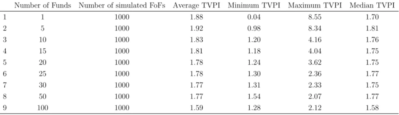
Table 11: Equal Rhythm: Results of buyout funds - TVPI

1 1 1000 1.88 0.04 8.55 1.70 2 5 1000 1.92 0.98 8.34 1.81 3 10 1000 1.83 1.20 4.16 1.76 4 15 1000 1.81 1.18 4.04 1.75 5 20 1000 1.78 1.24 3.62 1.75 6 25 1000 1.78 1.30 2.36 1.77 7 30 1000 1.77 1.31 2.33 1.75 8 50 1000 1.77 1.54 2.07 1.77 9 100 1000 1.59 1.28 2.12 1.58

Table 12: Equal Rhythm: Results of buyout funds - Other measures

1 1 0.8743 0.3399 0.0900 2.5831 14.0127 6.8404 2 5 0.5579 1.1079 0.0010 3.5067 27.1121 8.2295 3 10 0.3526 1.3190 0.0000 2.1051 7.3560 7.7781 4 15 0.3151 1.3440 0.0000 2.1871 7.8028 7.7768 5 20 0.2716 1.3614 0.0000 2.8111 14.4336 7.9130 6 25 0.1896 1.3588 0.0000 0.2337 0.1614 7.1132 7 30 0.1745 1.3727 0.0000 0.2419 0.2081 7.0910 8 50 0.0908 1.5862 0.0000 0.2292 -0.1137 7.1536 9 100 0.1100 1.3781 0.0000 1.2052 3.2075 6.7367

(42)

Table 13: Random Rhythm: Results of buyout funds - TVPI

1 1 1000 1.89 0.02 26.04 1.66 2 5 1000 1.83 0.91 11.26 1.69 3 10 1000 1.82 1.05 6.42 1.72 4 15 1000 1.80 1.07 6.10 1.70 5 20 1000 1.76 1.23 3.63 1.69 6 25 1000 1.76 1.25 3.34 1.70 7 30 1000 1.74 1.34 2.73 1.70 8 50 1000 1.71 1.38 2.26 1.70 9 100 1000 1.71 1.56 1.83 1.71

Table 14: Random Rhythm: Results of buyout funds - Other measures Number of Funds Standard deviation Worst 99th percentile Probability of a loss Skewness Kurtosis Utility 1 1 1.2502238 0.2500000 0.093 9.1209437 150.0552728 7.4586754 2 5 0.6664311 1.1156600 0.002 5.6836052 56.1702306 8.3306263 3 10 0.4356140 1.2410000 0.000 3.4719559 22.6261095 8.0513235 4 15 0.4321759 1.2806333 0.000 3.2074234 17.7173444 7.8824425 5 20 0.3036234 1.3414700 0.000 2.2315254 7.9658189 7.5924895 6 25 0.2868105 1.3675440 0.000 2.1754197 7.8843927 7.6007282 7 30 0.2130041 1.3849933 0.000 1.0617311 2.0447091 7.2276795 8 50 0.1516456 1.4038000 0.000 0.5144963 0.8883850 6.9798532 9 100 0.0524408 1.5957900 0.000 -0.0808798 -0.6320267 6.8003076

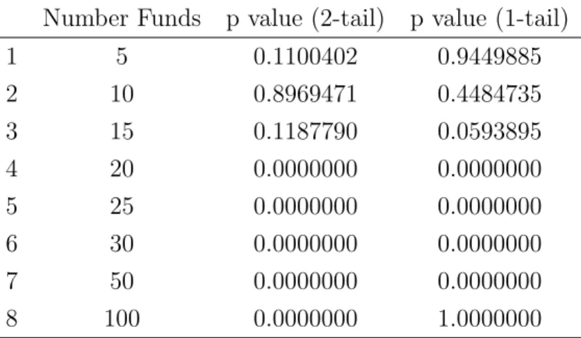
Table 15: Results of one- and two-sided MWW test, CI=95% (PERACS Risk Coefficient vs. Investment Rhythm)

Number Funds p value (2-tail) p value (1-tail)

1 5 0.1100402 0.9449885 2 10 0.8969471 0.4484735 3 15 0.1187790 0.0593895 4 20 0.0000000 0.0000000 5 25 0.0000000 0.0000000 6 30 0.0000000 0.0000000 7 50 0.0000000 0.0000000 8 100 0.0000000 1.0000000

with H1 : P ERACS Risk Coef f icientequal > P ERACS Risk Coef f icientrandom for

(43)

Tables 11 to 14 summarize the risk-return characteristics of both investment rhythms. I used buyout funds and venture capital funds with a 5-year investment period and equal portfolio weights. For both investment rhythms, the average TVPI first increases and then decreases, while the median TVPI gets closer to the average TVPI as n is increased. However, for the equal investment rhythm the average TVPI for n > 30 is reduced significantly from 2.04 (n = 25) to 1.59(n = 100).

I find that portfolios with random investment rhythm benefit more from adding funds to the portfolio than those with random investment rhythm. Firstly, the standard deviation of the TVPI for portfolios with random investment rhythm is higher for small number of funds. However, for n = 5 to n = 25, the standard deviation for portfolios with random investment rhythm is lower. Secondly, for an identical investment period, there is a lower return dispersion for portfolios with equally distributed vintage years when compared to randomly distributed vintage years. Nevertheless, figure 11 shows that, as n is increased, the return dispersion for portfolios with random investment rhythm is reduced signif-icantly and approximates the return dispersion of portfolios with an equal investment rhythm. This means that increasing diversification leads to an over-proportionate risk mitigating effect in portfolios with random investment rhythm. Intuitively, the simulated portfolios with a random investment rhythm enjoy a double-diversification effect: not only are more underlying funds added to the portfolio, but also the number of funds per vintage year are more diversified.

As the number of underlying funds is increased, the distributions of the PERACS Risk CoefficientTM become non-identical at a 0.05 significance level for n ≥ 20 (table 15). Interestingly, the one-tail MWW test reveals that the risk coefficient tends to be larger for equal investment rhythm portfolios only for 20 ≤ n ≤ 50. For those values, we can reject the null hypothesis and accept the hypothesis that the risk coefficient is larger for equal investment rhythm portfolios. For smaller and larger values of n, this holds not true.

Figure 14 shows that the optimal level of diversification is at 25 funds for portfolios with equal investment rhythm and 30 funds for portfolios with random investment rhythm. The maximum for the equal investment rhythm is higher, but is very close the maximum for the random investment rhythm. As n is increased, the number of investments per vintage year is relatively well diversified - even for the random investment rhythm.

(44)

1 5 10 15 20 25 30 50 100 0 5 10 15 20 25 30

Equal Rhythm TVPI distribution

Number of Funds TVPI 1 5 10 15 20 25 30 50 100 0 5 10 15 20 25 30

Random Rhythm TVPI distribution

Number of Funds TVPI 0.5 1.0 1.5 2.0

Standard deviation of Portfolio TVPI

Number of Funds Standard de viation 0.5 1.0 1.5 2.0

Standard deviation of Portfolio TVPI

Number of Funds Standard de viation 1 10 20 30 50 100 Investment Rhythm Equal Random 0 1 2 3 4 5 0.0 0.2 0.4 0.6 0.8 1.0 CDF by Investment Rhythm TVPI Fn(x) Weights Equal Random

(45)

0 2 4 6 8 10 Number of Funds Sk e wness 0 2 4 6 8 10 1 5 10 15 20 25 30 50 100 Investment Rhythm Equal Random

Figure 12: Skewness of portfolio TVPI vs. Number of Funds

0 50 100 150 Number of Funds K ur tosis 0 50 100 150 1 5 10 15 20 25 30 50 100 1 5 10 15 20 25 30 50 100 Investment Rhythm Equal Random

Figure 13: Excess kurtosis of portfolio TVPI vs. Number of Funds

(46)

6.0 6.5 7.0 7.5 8.0 8.5 9.0 Number of Funds Utility 6.0 6.5 7.0 7.5 8.0 8.5 9.0 1 5 10 15 20 25 30 50 100 Investment Rhythm Equal Random

Figure 14: Utility vs. Number of Funds

0 5 10 15 Number of Funds Risk−retur n r atio 0 5 10 15 1 5 10 15 20 25 30 50 100 1 5 10 15 20 25 30 50 100 Investment Rhythm Equal Random

Are Private Equity Funds of Funds managed by more risk-tolerant Private Equity Firms necessarily more risky?

Are Private Equity Funds of Funds managed by more

risk-tolerant Private Equity Firms necessarily more risky?

ABSTRACT OF THE MASTER THESIS

by

Torben Rabe

Master of Science in Management (Grande ´

Ecole)

HEC Paris, 2016

Professor Oliver Gottschalg, PhD

Are Private Equity Funds of Funds managed by more

risk-tolerant Private Equity Firms necessarily more risky?

Contents

List of Figures

List of Tables

Glossary

1

Introduction

2

Diversification

2.1

Private Equity and Modern Portfolio Theory

2.2

The Impact of Diversification on the Portfolio

2.3

The ”Optimal” Level of Diversification

2.4

How to achieve Diversification

3

Data

3.1

Data sample and Descriptive Statistics

3.2

Limitations of the dataset

3.3

Possible Biases

4

Framework & Model

4.1

Monte Carlo Simulation

4.2

Hypotheses

4.3

Measures

4.4

Other Measures

4.5

Limitations of the Model

5

Results

5.1

Hypothesis 1: Overall dataset and diversification level

5.2

Hypothesis 2: Investment period

5.3

Hypothesis 3: Investment rhythm