U.F.R. Sciences de la Vie et de la Terre
Thèse
pour obtenir le grade de
Docteur de l’Université de Toulouse
Délivré par l’Université Toulouse III – Paul Sabatier
Discipline : Neurosciences Cognitives
présentée et soutenue publiquement par
Timothée Masquelier
le 15 février 2008
Learning mechanisms to account for the
speed, selectivity and invariance of
responses in the visual cortex
Jury
Gustavo Deco
Rapporteur
Olivier Faugeras
Examinateur
Yves Frégnac
Rapporteur
Martin Giurfa
Examinateur
Pascal Mamassian Examinateur
There may be only a few basic learning mechanisms underlying all this complex [brain] activity. The final explanation is likely to be in terms of the basic patterns of connections laid down in normal development, plus the key learning algorithms that modify those connections and other neural parame-ters. Thus the neocortex may well have an underlying simplicity, not at the level at which the mature brain behaves but at the way by which it arrives at that intricate behavior, based on its innate structure and guided by its rich experience of the world.
In this thesis I propose various learning mechanisms that could account for the speed, selectivity and invariance of the neuronal responses in the visual cortex. I also present the results of a relevant psychophysical experiment demonstrating that familiarity can accelerate visual processing.
In Chapter 2, I demonstrate that, in a feedforward neural model of the ventral stream, a combination of a temporal coding scheme, where the most strongly activated neurons fire first, with Spike Timing Dependent Plasticity (STDP) leads to a situation where neurons in higher order visual areas will gradually become selective to frequently occurring feature combinations. At the same time, their responses become more and more rapid. I firmly believe that such mechanisms are a key to understanding the remarkable efficiency of the primate visual system.
In Chapter 3, I present a second study, not restricted to vision, where one receiving STDP neuron integrates spikes from a continuously firing neuron population. It turns out, somewhat surprisingly, that STDP is able to find repeating spatio-temporal spike patterns and to track back through them, even when embedded in equally dense ‘distractor’ spike trains – a computa-tionally difficult problem. STDP thus enables some form of temporal coding, even in the absence of an explicit time reference. Given that the mechanism exposed here is simple and cheap it is hard to believe that the brain did not evolve to use it.
One interesting prediction of the STDP models of Chapters 2 and 3 is that visual responses’ latencies should decrease after repeated presentations of a same stimulus. In Chapter 4 I tested this prediction experimentally by inferring the visual processing times through behavioral measures. I used a saccadic forced-choice paradigm. The target was always the same repeating image (an interior scene), while the distractors (other interior scenes) were changing. The experiment revealed a familiarity-induced speed-up effect of about 100 ms. Most of it can be attributed to the learning of the task but a ∼25 ms effect corresponds to the familiarity with a given image, and is reached after a few hundred presentations. Of course this does not mean
that the STDP models of Chapters 2 and 3 are true – only that they are plausible.
In Chapter 5, I investigated the learning mechanisms that could account for the invariance of certain neuronal responses to some stimulus proper-ties such as location or scale. It has been proposed that the appropriate connectivity could be learnt by passive exposure to smooth transformation sequences, and the use of a learning rule that takes into account the recent past activity of the cells: the ‘trace rule’. I proposed a new variant of the trace rule that only reinforces the synapses between the most active cells, and therefore can handle cluttered environments. I applied it on V1 complex cells in the HMAX model, and demonstrated that, after exposure to natural videos, the learning rule was indeed able to form pools of simple cells with the same preferred orientation but with shifted receptive fields.
Taken together, these simulations suggest how the visual cortex could wire itself. While still speculative at the time of writing the models presented here all rely on widely accepted biophysical phenomena and are thus biologically plausible. The psychophysical results of Chapter 4 are compatible with the STDP models of Chapter 2 and 3.
Those last two models also demonstrate how the brain could easily make use of information encoded in the spike times. Whether these spike times contain additional information with respect to the averaged firing rates – a theory referred to as ‘temporal coding’ – is controversial. Given that the mechanisms proposed here are simple, efficient, and satisfy the known tem-poral constraints coming from the experimental literature, they provide a strong argument in favor of the use of temporal coding, at least when rapid processing is involved.
Keywords: vision, object recognition, ultra-rapid visual categorization, learning, temporal coding, spiking neurons, Spike Timing Dependent Plas-ticity (STDP)
Dans cette thèse je propose plusieurs mécanismes d’apprentissage qui pourraient expliquer la rapidité, la sélectivité et l’invariance des réponses neuronales dans le cortex visuel. J’expose également les résultats d’une ex-périence de psychophysique pertinente, qui montrent que la familiarité peut accélérer les traitements visuels.
Au Chapitre 2, je démontre que, au sein d’un model neuronal de la voie ventrale de type ‘feedfoward’, la combinaison d’une part d’un schéma de codage temporel dans lequel les neurones les plus stimulés déchargent en premier, et d’autre part de la Spike Timing Dependent Plasticity (STDP), amène à une situation dans laquelle les neurones des aires de haut niveau deviennent graduellement sélectifs à des combinaisons fréquentes de primi-tives visuelles. En outre, les réponses de ces neurones deviennent de plus en plus rapides. Je crois fermement que de tels mécanismes sont à la base de la remarquable efficacité du système visuel du primate.
Au Chapitre 3 je présente une autre étude, non spécifique à la vision, dans laquelle un unique neurone reçoit des potentiels d’action (ou ‘spikes’) provenant d’une population d’afférents qui déchargent continuellement. Il s’avère, étonnamment, que la STDP permet de détecter puis de remonter des patterns de spikes spatio-temporels même s’ils sont insérés dans des trains de spikes ‘distracteurs’ de même densité – un problème computationnellement complexe. La STDP permet donc l’utilisation d’un codage temporel, même en l’absence d’une date de référence explicite. Etant donné que le mécanisme présenté ici est simple et peu coûteux, il est difficile de croire que le cerveau n’a pas évolué pour l’utiliser.
Une prédiction intéressante des modèles STDP des Chapitres 2 et 3 est que les latences des réponses visuelles devraient diminuer après présentations répétées d’un même stimulus. Au Chapitre 4 j’ai testé expérimentalement cette prédiction, en inférant les temps de traitement visuels à partir de me-sures comportementales. J’ai utilisé un paradigme de choix forcé saccadique, avec comme cible toujours la même image répétée (une scène d’intérieur), alors que les distracteurs (également des scènes d’intérieur) changeaient. Les
résultats mettent en évidence une accélération des temps de traitement de l’ordre de 100 ms. La majeur partie de cet effet est imputable à l’apprentis-sage de la tâche, mais environ 25 ms correspondent a de la familiarité avec une image donnée. Ces 25 ms sont gagnées au bout de quelques centaines de présentations. Bien sûr cela ne veut pas dire que les modèles STDP des Chapitres 2 et 3 sont vrais – seulement qu’ils sont plausibles.
Au Chapitre 5 j’ai recherché les mécanismes d’apprentissage qui pour-raient expliquer l’invariance de certaines réponses neuronales à certaines pro-priétés du stimulus visuel comme la position ou la taille. Il a été proposé que la connectivité appropriée pourrait être apprise à partir d’exposition passive à des séquences de transformations continues, et d’une règle d’apprentissage qui prend en compte l’activité de la cellule moyennée sur un passé récent : la ‘trace rule’. Je propose une nouvelle variante de cette ‘trace rule’ qui renforce uniquement les synapses entre les cellules les plus actives, ce qui lui permet de fonctionner dans des environnements chargés. Je l’ai appliquée sur les cellules complexes de V1 dans le modèle HMAX, et on voit que, après expo-sition à des vidéos naturelles, la loi d’apprentissage forme des ensemble de cellules simples dont l’orientation préférée est la même, mais dont les champs récepteurs sont décalés.
Les simulations présentées ici suggèrent comment le cortex visuel pourrait s’auto-organiser. Même s’ils sont spéculatifs aujourd’hui, les modèles propo-sés s’appuient tous sur des mécanismes biophysiques communément admis – ils sont donc biologiquement plausibles. Les résultats de psychophysique du Chapitre 4 sont compatibles avec les modèles STDP des Chapitres 2 et 3.
Ces deux derniers modèles démontrent aussi comment le cerveau pourrait facilement tirer profit de l’information contenue dans les dates de spikes. Si ces dates contiennent d’avantage d’information par rapport au taux de dé-charge moyen – la théorie dite du ‘codage temporel’ – est controversé. Etant donné que les mécanismes proposés ici sont à la fois simples, efficaces, et sa-tisfont les contraintes temporelles provenant de la littérature expérimentale, ils constituent un argument fort en faveur de l’utilisation de codage temporel, du moins dans les traitements rapides.
Mots-clefs : vision, reconnaissance d’objets, catégorisation visuelle ultra-rapide, apprentissage, codage temporel, neurones impulsionnels, Spike Ti-ming Dependent Plasticity (STDP)
I would like to acknowledge first my advisor Dr. Simon Thorpe (DR1 CNRS, France) for the quality of his supervision, his permanent enthusiasm, his creative ideas and his broad scientific curiosity. His open-mindedness pushed him to take me in his team although I had very little experience nor training in neuroscience.
I would like to thank all the team of SpikeNet Technology Inc. (http: //www.spikenet-technology.com/) for their support and for allowing me
to do both applied and fundamental research. In particular the
interac-tions with the R&D engineers Jong-Mo Allegraud and Nicolas Guilbaud were smooth and I think profitable for both parts. It was also a pleasure to work with them. I also acknowledge the Association Nationale pour la Recherche Technique (ANRT), which provided the other half of my funding through a Conventions Industrielles de Formation par la Recherche (CIFRE).
I would like to thank all the CERCO team for making the CERCO such a nice place to work, and in particular: Dr. Rufin Van Rullen (CR1 CNRS, France) for keeping an eye on my work, reading and commenting all my manuscripts before I submitted them, and giving me pointers to relevant lit-erature; my predecessor and collaborator Dr. Rudy Guyonneau who first in-troduced me to Spike Timing Dependent Plasticity; Sébastien Crouzet for his precious help on psychophysical issues; Dr. Jean-Michel Hupé (CR1 CNRS) for his expertise and rigor on statistics.
Many thanks to my friends and collaborators at MIT: Thomas Serre (Mc-Govern Institute, MIT), first – for convincing me to join the field of neuro-science, for the numerous brainstorms we had during my PhD, and for the profitable collaboration we had on invariance learning – and Prof. Tomaso Poggio (McGovern Institute, MIT) for welcoming me in his brilliant group in summer 2006 and spring 2007, and for the pertinent feedback he gave on my work.
I aknowledge the members of my thesis committee for their interest in my work: Prof. Dr. Gustavo Deco (ICREA, Spain), Dr. Olivier Faugeras (DR INRIA, France), Dr. Yves Frégnac (DR1 CNRS, France), Prof. Dr. Martin
Abstract iii
Résumé v
Acknowledgments vii
Contents xii
1 Introduction 1
1.1 Learning is the key . . . 1
1.2 Object recognition in the primate’s visual cortex . . . 3
1.2.1 Selectivity & invariance in the ventral stream . . . 3
1.2.2 Speed . . . 7
1.3 Learning and plasticity in the visual cortex . . . 10
1.4 Theoretical neuroscience . . . 11
1.4.1 Rate coding, temporal coding and population coding . 11 1.4.2 Randomness, noise, and unknown sources of variability 12 1.4.3 Neuronal models . . . 13
1.5 Evidence for temporal coding in the brain . . . 15
1.6 Models of object recognition in cortex . . . 17
1.6.1 Feedforward and feedback . . . 17
1.6.2 Static, single spike wave and mean field approximations 19 1.6.3 Weight-sharing . . . 20
1.7 Spike Timing Dependent Plasticity (STDP) . . . 21
1.7.1 Experimental evidence . . . 21
1.7.2 Previous modeling work . . . 22
1.8 Original contributions . . . 24
1.8.1 STDP-based visual feature learning . . . 24
1.8.2 STDP-based spike pattern learning . . . 26
1.8.3 Visual learning experiment . . . 26
1.8.4 Invariance learning . . . 27 ix
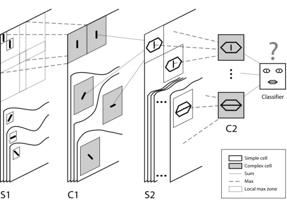
2 STDP-based visual feature learning 29 2.1 Résumé . . . 29 2.2 Abstract . . . 30 2.3 Introduction . . . 31 2.4 Model . . . 32 2.4.1 Hierarchical architecture . . . 32 2.4.2 Temporal coding . . . 32 2.4.3 STDP-based learning . . . 34 2.5 Results . . . 35 2.5.1 Single-class . . . 36 2.5.2 Multi-class . . . 40 2.5.3 Hebbian learning . . . 43 2.6 Discussion . . . 45
2.6.1 On learning visual features . . . 45
2.6.2 A bottom-up approach . . . 46
2.6.3 Four simplifications . . . 46
2.6.4 ‘Early vs. later spike’ coding and STDP: two keys to understand fast visual processing . . . 48
2.7 Technical details . . . 49 2.7.1 S1 cells . . . 50 2.7.2 C1 cells . . . 50 2.7.3 S2 cells . . . 51 2.7.4 C2 cells . . . 51 2.7.5 STDP Model . . . 51 2.7.6 Classification setup . . . 52 2.7.7 Hebbian learning . . . 53
2.7.8 Differences from the model of Serre, Wolf and Poggio . 54 3 STDP-based spike pattern learning 55 3.1 Résumé . . . 55
3.2 Abstract . . . 56
3.3 Introduction . . . 57
3.3.1 The computational problem: spike pattern detection . 57 3.3.2 Background: STDP and discrete spike volleys . . . 57
3.3.3 Experimental set-up: STDP in continuous regime . . . 59
3.4 Results . . . 60
3.4.1 A first example . . . 60
3.4.2 Batches . . . 64
3.5 Discussion . . . 69
3.5.1 STDP in continuous regime . . . 69
3.5.3 Argument for temporal coding . . . 70
3.5.4 A generic mechanism . . . 71
3.5.5 Extension: competitive scheme . . . 71
3.6 Technical details . . . 72
3.6.1 Poisson spike trains . . . 72
3.6.2 Leaky Integrate and Fire (LIF) neuron . . . 73
3.6.3 Spike Timing Dependent Plasticity . . . 75
4 Visual learning experiment 77 4.1 Résumé . . . 77
4.2 Abstract . . . 78
4.3 Introduction . . . 78
4.4 Methods . . . 80
4.4.1 Participants . . . 80
4.4.2 The saccadic forced-choice . . . 80
4.4.3 Design . . . 81
4.4.4 Stimuli . . . 82
4.4.5 Saccade detection . . . 83
4.5 Results . . . 84
4.6 Discussion . . . 90
4.6.1 A robust experience-induced speed-up . . . 90
4.6.2 Type of stimuli and shift-invariance . . . 90
4.6.3 Target-distractor distance has more impact than intra-class variability . . . 91
4.6.4 The gap shifts the speed-accuracy trade-off . . . 93
4.7 Conclusion . . . 93
5 Invariance learning: a plausibility proof 95 5.1 Résumé . . . 95
5.2 Abstract . . . 97
5.3 Introduction . . . 98
5.4 HMAX Model . . . 99
5.4.1 The Simple S units . . . 99
5.4.2 The Complex C units . . . 99
5.4.3 Neural implementations of the two key operations . . . 101
5.5 On learning correlations . . . 103
5.5.1 Simple cells learn spatial correlations . . . 103
5.5.2 Complex cells learn temporal correlations . . . 104
5.6 Results . . . 107
5.6.1 Simple cells . . . 107
5.7 Discussion . . . 110
5.8 Technical details . . . 114
5.8.1 Stimuli: the world from a cat’s perspective . . . 114
5.8.2 LGN ON- and OFF-center unit layer . . . 115
5.8.3 S1 layer: competitive hebbian learning . . . 115
5.8.4 C1 Layer: pool together consecutive winners . . . 117
5.8.5 Main differences with Einhäuser et al . 2002 . . . 118
6 Conclusions 119 6.1 Résumé . . . 119
6.2 On selectivity, invariance and speed in the visual system . . . 121
6.3 On learning rates . . . 122
6.4 On temporal coding in general . . . 122
6.5 Perspective: top-down effects and feedback . . . 123
6.6 On the roles of models . . . 123
6.7 Applications . . . 124
A Papers (Peer-reviewed international journals) 127 A.1 Unsupervised Learning of Visual Features through Spike Tim-ing Dependent Plasticity . . . 127
A.2 Spike Timing Dependent Plasticity Finds the Start of Repeat-ing Patterns in Continuous Spike Trains . . . 139
B Conference abstracts & posters 149 B.1 Ultra-rapid visual form analysis using feedforward processing . 149 B.2 Face feature learning with Spike Timing Dependent Plasticity 150 B.2.1 Paper . . . 150
B.2.2 Poster . . . 155
B.3 Learning simple and complex cells-like receptive fields from natural images: A plausibility proof . . . 157
B.3.1 Abstract . . . 157
B.3.2 Poster . . . 157
List of tables 159
List of figures 167
Introduction
1.1
Learning is the key
Activity driven refinement of local neural networks, through synaptic plastic-ity and axon remodeling, is ubiquitous in developing neural systems, and is a necessary supplement to the genetically programmed mechanism of laying out coarse connections between brain areas (Katz and Shatz, 1996; Innocenti and Price, 2005). In some cases, this refinement must occur at a given period of development, said ‘critical’, otherwise the functionality of the network is irreversibly impaired. For example Hubel and Wiesel demonstrated that ocu-lar dominance columns in the lowest neocortical visual area of cats, V1, were largely immutable after a critical period in development (Hubel and Wiesel, 1970). In congenitally blind people, the areas that would have become visual are involved in other functions, such as audition or language processing (see for example (Ofan and Zohary, 2007)). This means that an area ’s functions largely emerges from experience, and are not hard-coded in the genes.
Among all the living organisms humans are probably the ones that learn the most. New born humans are far from being operational and need con-stant education and care for at least the first ten years of their lives. Wild children’s development is severely impaired and lead to irreversible disfunc-tions (Benzaquén, 2006). At birth our brain volume is only 25% of its adult size (against 70% in the macaque). Most of the cerebral growth thus occurs after birth, while the organism is perceiving the outside world, and interact-ing with it. The acquisition of cognitive skills, and the underlyinteract-ing cerebral maturation and brain area specialization, thus result from complex interac-tions between experience and a genetically specified assembly program.
The cost of the long necessary training for humans is probably compen-sated by the ability to adapt to new environments and to build on knowledge
acquired by others, in particular across generations. This contrasts with more primitive organisms, which are genetically programmed to behave in a more fixed manner, but need less training.
From a computational point of view learning is arguably the key to un-derstanding intelligence (Poggio and Smale, 2003), and has thus been studied extensively by the Artificial Intelligence community. In the context of neural networks learning can be defined as follow (Haykin, 1994):
Learning is a process by which the free parameters of a neural network are adapted through a process of stimulation by the environment in which the network is embedded. The type of learning is determined by the manner in which the parameter changes take place.
Among all the potential parameters the synaptic weights are probably the most important. In the cortex the number of connections from and to each neuron is in the order of a few thousands, and activity-driven synaptic reg-ulation has been observed both in vivo and in vitro. The key of intelligence probably lies in this dense connectivity and its plasticity.
We distinguish supervised and unsupervised learning. Supervised learn-ing requires a ‘teacher’, and is task-specific. For example a network can be trained to classify between faces and non-faces images from a set of labeled examples. The network is then able to generalize to new data to a certain extent, that is to label previously unseen images. This capacity to generalize, beyond the memory of specific examples, is critical (Poggio and Bizzi, 2004). Vapnik and Chervonenkis showed that there is an optimal VC dimension for the network (Vapnik and Chervonenkis, 1971) (the VC dimension is roughly the capacity of the network to fit any set of training data). If it is too small the network is not flexible enough to learn the training examples, let alone to generalize. If it is too big the network behaves like a look-up table: it does learn the specific training associations but does not generalize well to new data, unless a huge amount of training data is available. Humans, by being able to learn a new visual category from just a few examples, clearly outperform any machine-learning algorithm today. How we generalize so well remains a mystery.
In unsupervised (or self-organized) learning there is no external teacher to oversee the learning process. However, providing the world is not random, the network can tune itself to its statistical regularities. It can develop the ability to form internal representations for encoding features of the input and thereby to create new classes automatically (Becker, 1991). This type of learning is task-independent: it only depends on the world’s statistics. Unsupervised learning presumably dominates in the lower layers of the visual
system.
1.2
Object recognition in the primate’s visual
cortex
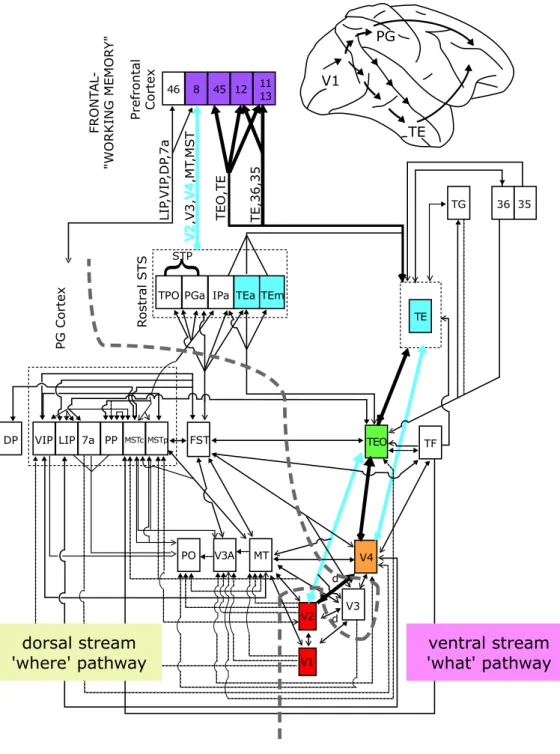
The primate’s visual cortex processes the information coming from the retina through the Lateral Geniculate Nucleus (LGN). It is made of several areas that are roughly hierarchically organized (Felleman and Van Essen, 1991). As can be seen on Fig. 1.1, it is generally assumed that the processing can be divided in two pathways: the so-called ventral and dorsal streams (Mishkin et al., 1983; DeYoe and Essen, 1988). The first one, also called the ‘what’ pathway, is primarily involved in object recognition (independently of the object location), whereas the second one, also called the ‘where’ pathway is mostly involved in spatial vision, object localization, and control of ac-tion (Ungerleider and Haxby, 1994). From now on I am going to focus on the ventral stream, which consists in a chain of neurally interconnected areas, including the primary visual cortex V1, and the extrastriate visual areas V2, V4 and IT.
Beyond IT, the Pre-Frontal Cortex (PFC) is thought to be involved in
linking perception to memory and action. It is probably there that the
categorization take place, essentially from the output of IT, using task specific circuits (Freedman et al., 2001).
1.2.1
Selectivity & invariance in the ventral stream
Robust object recognition requires both selectivity – so that an object (or object class) A is not confused with an object (class) B – and invariance – so that the object (class) A is recognized whatever its position, scale and whatever the viewpoint and lighting conditions, and eventually despite non-rigid transformations (for example facial expressions) and, for categorization, variations of shape within a class. Computer vision scientists know well how difficult this problem is. For example two face portraits of two individuals A and B are usually much more similar, in terms of low level image features, than a face and a profile portrait of A. Yet our visual system robustly extracts the identity the people in our visual fields, outperforming any computer vision system. How do we do that?
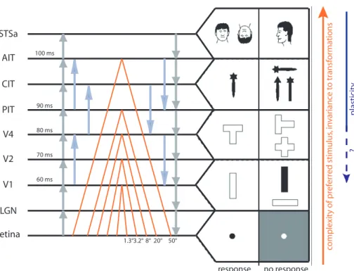
Over the last decades, a number of physiological studies in non-human primates have established several basic facts about the cortical mechanisms of recognition in the ventral stream. The accumulated evidence points towards two key features (see Fig. 1.2): from V1 to IT, there is a parallel increase in:
}
PG Cortex Ro s tr al ST S Prefrontal Cortex STP FRONT AL -"WORKING MEMOR Y" DP VIP LIP 7a PP FST PO V3A MT TPO PGa IPaV3 V4 TEO TF TG LIP ,VIP ,DP ,7a V2 ,V3, V4 ,MT ,MST TEO ,TE TE,36,35 MSTc d d V1 PG TE 46 8 45 12 11 13 TEa TEm TE V2 V1 dorsal stream 'where' pathway ventral stream 'what' pathway MSTp 35 36
Figure 1.1: Ventral and dorsal streams of the visual cortex. Modified from Ungerleider & Van Essen (Gross, 1998). Courtesy of Thomas Serre.
retina 60 ms LGN V1 V2 V4 PIT CIT AIT STSa response no response co m p le xi ty o f p re fe rr ed s ti m u lu s, in va ri an ce to t ra n sf o rm at io n s p la st ic it y ? 1.3°3.2° 8° 20° 50° 70 ms 80 ms 90 ms 100 ms
Figure 1.2: Increasing selectivity, RF sizes, and response latencies along the ventral stream. Modified it from (Oram and Perrett, 1994; Serre et al., 2007). Typical latencies are from (Thorpe and Fabre-Thorpe, 2001). RF sizes are from (Wallis and Rolls, 1997)
1. the complexity of the optimal stimuli for the neurons (Perrett and Oram, 1993; Desimone, 1991; Kobatake and Tanaka, 1994). That is neurons respond selectively to objects that are more and more complex. To be precise, V1 neurons’ preferred stimuli are oriented bars (Hubel
and Wiesel, 1959, 1968). In V2 many neurons are also orientation
selective (Hubel and Wiesel, 1965, 1970) but some encode combina-tions of orientacombina-tions such as angles (Boynton and Hegdé, 2004; Anzai et al., 2007). Further along in the hierarchy, neurons in V4 respond to features of intermediate complexity (Kobatake et al., 1998), such as Cartesian and non-Cartesian gratings (Gallant et al., 1996) or combi-nation of boundary conformations (Pasupathy and Connor, 1999, 2001, 2002). Beyond V4, in the Infero-Temporal cortex (IT), and particularly in its anterior part (AIT) neurons are tuned to complex stimuli, for ex-ample faces, hands and other body parts (Gross, 1972; Bruce et al., 1981; Perrett et al., 1982; Rolls, 1984; Perrett et al., 1984; Baylis et al., 1985; Perrett et al., 1987; Yamane et al., 1988; Hasselmo et al., 1989; Perrett et al., 1991, 1992; Hietanen et al., 1992; Souza et al., 2005), see (Logothetis and Sheinberg, 1996) for a review.
2. invariance of the responses to position and scale (Hubel and Wiesel, 1968; Perrett and Oram, 1993; Logothetis et al., 1995; Logothetis and Sheinberg, 1996; Tanaka, 1996; Riesenhuber and Poggio, 1999), and finally view point (Logothetis et al., 1995). This also means the size of the Receptive Fields (RF) increases until IT (Perrett and Oram, 1993; Tanaka, 1996). Understanding how these invariances are obtained – while neurons remain selective to their preferred stimuli – is a major challenge for visual neuroscientists. In V1, Hubel and Wiesel identified two kinds of cells that differ in their functional properties: the simple and the complex cells (Hubel and Wiesel, 1968). Both are orientation selective, but the complex cells’ responses are more invariant to the phase and/or position of the stimuli. To account for this invariance, Hubel and Wiesel (1962) proposed that the complex cells could pool their inputs from a group of simple cells tuned to the same orientation, but with shifted receptive fields. A number of models have been built on this proposal, extending the scheme to the whole hierarchy (Fukushima, 1980; LeCun and Bengio, 1998; Riesenhuber and Poggio, 1999; Wallis and Rolls, 1997; Rolls and Milward, 2000; Stringer and Rolls, 2000; Masquelier and Thorpe, 2007; Serre et al., 2007). How the appropriate connectivity could be learnt remains largely unknown and is the subject of Chapter 5. Lastly, one of the most striking aspect of the the shift and scale invariance observed in higher area such as IT is that it does not
seem to require exhaustive previous experience (Logothetis et al., 1995; Hung et al., 2005). Show a monkey an object it has never seen before at position P and scale S. This generates a set of IT responses R. Shifting
the object by a few degrees (∼4◦ for typical stimulus size of 2◦ ) or
rescaling it by a few octaves (∼2) will generate a new set of responses
R0 similar to R. Whether such invariance derives from a lifetime of
previous experience with other similar objects (feature sharing) or from innate structural properties of the visual system or both, remains to be determined. In any case, the observation that the adult IT population has significant position and scale invariance for arbitrary ‘novel’ objects provides a strong constraint for any explanation of the computational architecture and function of the ventral visual stream (Hung et al., 2005).
1.2.2
Speed
The speed of object recognition in cortex is an extremely useful piece of in-formation since it allows to infer what could be the underlying neural compu-tations and to exclude some type of processing that are too time-consuming. The visual system seems to have an ‘fast recognition’ mode – the initial phase of recognition before eye movements and high-level processes can play a role – which is already surprisingly accurate. This ‘fast recognition’ has been studied extensively in humans and monkeys by Thorpe and colleagues us-ing ultra-rapid categorization paradigms (Thorpe et al., 1996; Fabre-Thorpe et al., 1998; Rousselet et al., 2002; Bacon-Mace et al., 2005; Kirchner and Thorpe, 2006; Girard et al., 2007). Recently, it has been found that when two images are simultaneously flashed to the left and right of fixation, human subjects can make reliable saccades to the side where there is a target animal in as little as 120-130 ms (Kirchner and Thorpe, 2006). If we allow 20-30 ms for motor delays in the oculomotor system, this implies that the underlying visual processing can be done in 100 ms or less. The same protocol has just been used with monkeys, leading to even faster minimal reaction times of about 100 ms (Girard et al., 2007). Fig. 1.3 illustrates the time course of visual and motor processing in a go-no go task.
This psychophysical result is backed-up by electrophysiology in monkeys. The responses in IT begin 80-100 ms after onset of the visual stimulus, and are selective from the very beginning (Oram and Perrett, 1992), here to faces and heads, even in Rapid Serial Visual Presentation (RSVP) paradigms, when the preferred image is hidden in a continuous flow at rates up to 72
images per seconds (Keysers et al., 2001). More recently, recordings in
pro-Figure 1.3: The feedforward circuits involved in a go-no go rapid visual categorization task in monkeys. At each stage two latencies are given: the first is an estimate of the earliest neuronal responses to a flashed stimulus, whereas the second provides a more typical average latency. Reproduced with permission from (Thorpe and Fabre-Thorpe, 2001)
LGN V1 V2 V4 IT
20-40ms 30-50ms 40-60ms 50-70ms 60-80ms 70-100ms Retina
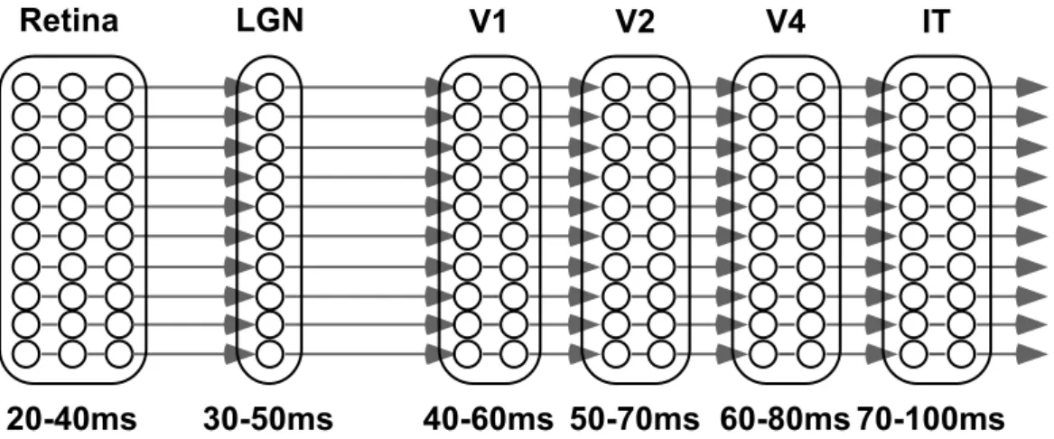
Figure 1.4: Constraints on computation time in an ultra-rapid visual
cat-egorization task (adapted from (Thorpe and Imbert, 1989)). The shortest path from the retina to IT has at least 10 neuronal layers. At each stage two latencies are given: the first is an estimate of the earliest neuronal responses to a flashed stimulus, whereas the second provides a more typical average la-tency. The time window available for a neuron to perform its computation is in the order of 10 ms, and will rarely contain more than one spike. Feedback is almost certainly ruled out.
duce essentially a binary vector with either ones or zeros) and only about 100 ms after stimulus onset contain remarkably accurate information about the nature of a visual stimulus (Hung et al., 2005).
These temporal constraints are extremely severe: given than about 10 neuronal layers separate IT from the retina (see Fig. 1.4), they leave about 10 ms of processing time for each neuron (Thorpe and Imbert, 1989). Since firing rates are seldom above 100 Hz in the visual system, this 10 ms window will rarely contain more than one spike. So talking about the firing rate of one neuron in this ‘fast recognition’ mode makes little sense, though we can talk about the firing rate of a population of neurons (see also 1.4.1). We can also talk about individual spike times. These spike times have been largely ignored by most of the neuroscientists: since Adrian recorded sensory neurons in the 1920’s and reported that their mean firing rates increased with the intensity of the stimulus (Adrian, 1928) it has been commonly assumed that these rates encode most of the information. However this view is under challenge, as we will see in Section 1.3.
These severe temporal constraints have another major implication: they almost certainly rule feedback out (see Fig. 1.4), and suggests that a core hi-erarchical feedforward architecture may be a reasonable starting point for
a theory of visual cortex aiming to explain ‘fast recognition’. This
hy-pothesis is backed up by the fact that feedforward-only models have been shown to perform very well on object recognition in natural non-segmented images (Masquelier and Thorpe, 2007; Serre et al., 2007), sometimes even matching the human performance with backward masking (Serre et al., 2007).
1.3
Learning and plasticity in the visual cortex
In the developing animal, ‘rewiring’ experiments (see (Horng and Sur, 2006) for a recent review), which re-route inputs from one sensory modality to an area normally processing a different modality, have now established that visual experience can have a pronounced impact on the shaping of cortical networks. How plastic is the adult visual cortex is however still a matter of debates.
From the computational perspective, it is very likely that learning may occur in all stages of the visual cortex. For instance if learning a new task involves high-level object-based representations, learning is likely to occur high-up in the hierarchy, at the level of IT or PFC. Conversely, if the task to be learned involves the fine discrimination of orientations like in perceptual learning tasks, changes are more likely to occur in lower areas at the level of V1, V2 or V4 (see (Ghose, 2004) for a review). It is also very likely
that changes in higher cortical areas should occur at faster time scales than changes in lower areas.
By now there has been several reports of plasticity in all levels of the ventral stream of the visual cortex (see (Kourtzi and DiCarlo, 2006), i.e. both in higher areas like PFC (Rainer and Miller, 2000; Freedman et al., 2003;
Pasupathy and Miller, 2005) and IT (see for instance (Logothetis et al.,
1995; Rolls, 1995; Kobatake et al., 1998; Booth and Rolls, 1998; Erickson et al., 2000; Sigala and Logothetis, 2002; Baker et al., 2002; Jagadeesh et al.,
2001; Freedman et al., 2006) in monkeys or the LOC in humans (Dolan
et al., 1997; Gauthier et al., 1999; Kourtzi et al., 2005; Op de Beeck et al., 2006; Jiang et al., 2007). Plasticity has also been reported in intermediate areas like in V4 (Yang and Maunsell, 2004; Rainer et al., 2004) or even lower areas like V1 (Singer et al., 1982; Karni and Sagi, 1991; Yao and Dan, 2001; Schuett et al., 2001; Crist et al., 2001), although their extent and functional significance is still under debate (Schoups et al., 2001; Ghose et al., 2002; DeAngelis et al., 1995).
Supervised learning procedures to validate Hebb’s covariance hypothesis in vivo in the visual cortex at the cellular level have also been proposed. The covariance hypothesis predicts that a cell’s relative preference between two stimuli could be displaced towards one of them by pairing its presentation with imposed increased responsiveness (through iontophoresis). It was indeed shown possible to durably change some cells’ RF properties in cat primary visual cortex, such as ocular dominance, orientation preference, interocular orientation disparity and ON or OFF dominance, both during the critical developmental period (Frégnac et al., 1988) and in adulthood (McLean and Palmer, 1998; Frégnac and Shulz, 1999). More recently, a similar proce-dure was used to validate the Spike Timing Dependent Plasticity (see Sec-tion 1.7.1) in developing rat visual cortex (Meliza and Dan, 2006) using in vivo whole-cell recording.
Altogether the evidence suggests that learning plays a key role in deter-mining the wiring and the synaptic weights of visual cortex cells.
1.4
Theoretical neuroscience
1.4.1
Rate coding, temporal coding and population
cod-ing
Where neural information processing is concerned, it is usually assumed that spikes are the basic currency for transmitting information between neurons, the reason being that they can propagate over large distances. How the brain
actually uses them to encode information remains more controversial. Spikes have little variation in amplitude and duration (about 1 ms). They are thus fully characterized by their dates (the idea that this spike dates indeed contain information is referred to as ‘temporal coding’). However many electrophysiologists report that the individual dates are not always reliable. Summarizing them by counting how many spikes occurred in a given time window (i.e. computing a mean firing rate) usually leads to more reproducible values. Whether information is lost in this averaging operation has been the object of an on going debate for some time. (the idea that most of the information remains in the averaged rate is referred to as ‘rate coding’).
The answer probably depends on the size of the time window. If too big, averaged values may fail to capture some dynamical aspects of the re-sponses. It is thus tempting to use a small window, and compute a more ‘instantaneous’ firing rate. However to estimate the firing rate of one neu-ron the time window must contain at least a few spikes. The minimal time window is thus in the order of a few typical Inter Spike Intervals (ISI). This is sometimes longer than the order of magnitude of some behavioral times, ruling out the hypothesis that the individual firing rates are indeed used in the neural computations that underlie the behavior.
Electrophysiologists can sometimes reduce this window by averaging over several runs, with carefully controlled conditions. Obviously this solution is not possible in the brain. However the same result could be obtained by averaging over a population of redundant neurons with similar selectivity. This is referred to as ‘population coding’ and is indeed a possibility, though costly in terms of number of neurons (Gautrais and Thorpe, 1998).
In this thesis, I explored another possibility. I assumed individual spike times were (somewhat) reliable, despite what some electrophysiologists think, and investigated how information could be encoded and decoded in those spike times.
1.4.2
Randomness, noise, and unknown sources of
vari-ability
According to Laplace, randomness is only a measure of our “ignorance of the different causes involved in the production of events.” (Laplace, 1825). Throw a dice. You cannot guess the number that will come out. But theoretically, if you knew the initial conditions (speed and position of the dice) with enough precision, and used an fine enough model, you could compute it. The more chaotic the system (high sensitivity to the initial conditions), the more you
need to know the initial conditions with accuracy. Now build a machine capable to throw the dice always at the same position and speed. If the machine is accurate enough, the the number which comes out will always be the same. Thus the dice by itself is not a random number generator.
Whether we live in a deterministic world or not, and the implications for the notion of free will, have been the object of a raging debate for some centuries, involving both scientists and philosophers. It is out of the scope of this thesis. However there is generally a consensus on that in realistic experiences there is always a limit on how accurately controlled the conditions are, and there are usually non-controlled ones. Both can lead to unexplained variability in the results that we call ‘noise’ (even though the term can be misleading and I prefer the term ‘unexplained variability’).
In the field of neuroscience, this variability is huge. According to the semi-serious Harvard Law of Animal Behavior: “Under carefully controlled experimental circumstances, an animal will behave as it damned well pleases”. Electrophysiologists also report variability in their measures. But inferring a lack of precision in the neural code from observations of variability is haz-ardous. In this thesis, I will argue that the variability in some recorded spike times, in particular in the visual system, could come from non-controlled variables that might also affect neuronal activation, such as attention, eye movements, mental imagery, top-down effects etc. This is even more true for higher order neurons, because they do not only receive input from the retina, so the total input for these neurons is basically unknown. As Barlow wrote about neural responses in 1972, “their apparently erratic behavior was caused by our ignorance, not the neuron’s incompetence.” (Barlow, 1972).
1.4.3
Neuronal models
Computational neuroscientists have come-up with more or less detailed neu-ronal models. At which level the neurons should be modeled in a neural network model is always a difficult question. The neuronal model should capture all the essential mechanisms that underlie the network’s functional-ity, and, to save time, avoid computing side effects which do not impact this functionality. This is easier said than done.
A somewhat coarse model is the firing rate model. It is an approximation
of how a neuron behaves in a steady regime. The input spikes are then
summarized by a firing rate xj for each afferent (it thus ignores, among
other things, that simultaneous presynaptic spikes are more efficient than distant ones in triggering a postsynaptic one). The output spikes are also
summarized as a firing rate y, given by: y = f X j wj · xj ! (1.1)
f is the transmission function that is increasing and usually non-linear. In particular f usually saturates above a certain value, because the output firing rate is limited by the refractory period. A popular choice for f is a sigmoid. This model, although very simplified, is extremely popular, in particular among the Artificial Intelligence community. For example the well known perceptron or the Self-Organizing Maps (SOM) both use rate-based neuronal models.
In the firing rate model the individual spikes are not modeled. When needed, some authors sometimes generate them through a stochastic process (usually Poisson). The existence of such randomness in the true spike gener-ation process is somewhat dubious, especially because we know that neurons stimulated directly by current injection in the absence of synaptic input give highly stereotyped and precise responses (Mainen and Sejnowski, 1995).
Another drawback of the firing rate model is the assumption of a steady regime. It thus fails to capture the transients, which are probably the most interesting aspects of neural computation, especially when rapid processing is involved.
For these reasons, in most the work presented here I have used the (Leaky) Integrate-and-Fire model, in which individual input and output spikes are modeled. A neuron is modeled as a capacitor C in parallel with a leaking resistance R driven by an input current I(t). The membrane potential u is thus driven by:
C · du
dt = I(t) −
u(t)
R (1.2)
If we multiply Eq. 1.2 by R and introduce the membrane time constant
τm = RC of the leaky integrator, it follows:
τm·
du
dt = R · I(t) − u(t) (1.3)
If the input current I(t) is in fact generated by the arrival of presynaptic
spikes s at several synapses indexed by j, with weights wj, and at times t
(s) j
it has the form:
I(t) =X j wj · X f α(t − t(s)j ) (1.4)
and that we will not detail here.
The LIF neuron also has a threshold. When it is reached, due to the nearly simultaneous arrival of several presynaptic spikes, a postynaptic spike is emitted. This is followed by a negative after potential and a refractory period, during which the membrane potential is set to a resting value. Then Eq. 1.3 holds again. Fig. 1.5 illustrates those points.
Finer biophysical neuronal models also exists such as conductance-based IF (gIF) models (Destexhe, 1997), the Hodgkin-Huxley model (Hodgkin and Huxley, 1952) or compartmental models (see (Brette et al., 2007) for a recent review on spiking neuron models). They provide a detailed description of how one single neuron behaves, but their computational cost is usually prohibitive for network applications like the ones I investigate in this thesis. The LIF model is widely accepted as a decent approximation of real neurons and I assumed it did capture all the essential mechanisms.
1.5
Evidence for temporal coding in the brain
Since Adrian recorded sensory neurons in the 1920’s and reported that their mean firing rates increased with the intensity of the stimulus (Adrian, 1928) it has been commonly assumed that these rates encode most of the informa-tion processed by the brain. According to this view the spike generainforma-tion is supposed to be a stochastic process, usually assumed to be Poisson. The sig-nature of such a Poisson process is that the spike count over a time interval has a variance equal to its mean across trials (the ratio of both quantities is called the Fano factor and it thus equal to 1 for a Poisson process).
However the conventional view is under challenge. First various recent studies show that some neuronal responses are too reliable for the Poisson hypothesis to be tenable: for example Liu et al. (2001) and (Uzzell and Chichilnisky, 2004) find a Fano factor of about 0.3 in the retina and in the LGN respectively. Amarasingham et al. (2006) also proves that the Poisson hypothesis should be rejected for the first part of IT responses, from 100 ms to 300 ms after stimulus onset.
Second spike times are found reproducible in many neuronal systems (see Table 1.1), sometimes with millisecond precision. The time reference is either the onset of a stimulus, the maximum of a brain oscillation, or other spike times in case of spike patterns. These spike times are shown to encode infor-mation, sometimes complementary with respect to the information encoded in the rates: for example in monkeys Gawne et al. (1996) found that some V1 neurons encode the stimulus form in their rates and the stimulus contrast in their latency, and Kiani et al. (2005) showed that IT responses’ latencies
0 10 20 30 40 50 60 70 80 −3 −2 −1 0 1 2 3 4 5 6 t(ms)
Potential (arbitrary units)
potential threshold resting pot. input spike times
Figure 1.5: Leaky Integrate-and-Fire (LIF) neuron. Here is an illustrative example with only 6 input spikes. The graph plots the membrane potential as a function of time, and clearly demonstrates the effects of the 6 corresponding Excitatory PostSynaptic Potentials (EPSP). Because of the leak, for the threshold to be reached the input spikes need to be nearly synchronous. The LIF neuron is thus acting as a coincidence detector. When the threshold is reached, a postsynaptic spike is fired. This is followed by a refractory period of 1 ms and a negative spike-afterpotential.
were shorter for human faces than for animal faces, although both resulted in the same response magnitude.
In spontaneous activity, several second long firing sequences have also been found reproducible in slices of mouse primary visual cortex or in intact cat primary visual cortex in vivo (Ikegaya et al., 2004). Such long sequences, called ‘cortical songs’, could be generated by synfire chains (Abeles, 2004), that is series of pools of neurons connected in a feedforward manner. Note that the relevance of such long cortical songs in vivo is controversial because they could emerge by chance (McLelland and Paulsen, 2007; Mokeichev et al., 2007). However the spikes of the first 100 ms after the onset of an active period (‘UP state’) occur with up to millisecond precision (Luczak et al., 2007).
Other authors report a higher variability in the spike times. But first the variability could also come from the use of an inappropriate time reference. For example the stimulus onset is often used, while using the population ac-tivation onset (i.e. measuring the relative neuron’s latency with respect to its neighbors) sometimes lead to more reproducible and informative values Chase and Young (2007). This of course requires simultaneous multi-units record-ing. When oscillations are present, using their maximums as a time reference (i.e. measuring the phase of the spikes) may lead to more reproducible values than the absolute latencies. For example Fries et al. (2001) recorded neu-rons in cat primary visual cortex and showed that their absolute latencies could be prolonged or shortened from one trial to another (depending on when the stimulus was presented with respect to the phase of a LFP gamma-oscillation) but their phase with respect to the gamma-cycle reference frame remained roughly constant (Fries et al., 2007).
Second, as said above in Section 1.4.2, such variability, could come from non-controlled variables.
1.6
Models of object recognition in cortex
1.6.1
Feedforward and feedback
The vast majority of models of object recognition in cortex today are feedfor-ward only, and ignore back-projections (Fukushima, 1980; LeCun and Ben-gio, 1998; Riesenhuber and PogBen-gio, 1999; Wallis and Rolls, 1997; Rolls and Milward, 2000; Stringer and Rolls, 2000; Ullman et al., 2002; Masquelier and Thorpe, 2007; Serre et al., 2007). This is somewhat surprising as the circuitry of the cortex involves a massive amount of backprojections that convey infor-mation from higher areas back to the lower areas (Felleman and Van Essen,
T a ble 1 .1 : Evid en ce for temp o ra l co di ng in the brain (ada pt ed and up dated fro m (V anRullen et a l., 2 005 )) Sy stem/Prep ara tion Reco rdin g si te Co d ing In format ion Ref erence sign al Ref s So m a tosen sory Human P eripheral nerv e fib ers Time -to-first-spik e Direction of force, surface shap e Stim ulus o nset Joh ansson and Birznieks (2004) Ra t Barrel cortex T ime-to-fi rst-spik e (inhi bition ba rra ge) Stim ulus lo cat ion Stim ulus o nset P etersen et al. (2001); Sw a dlo w and G usev (2002) Ra t Prim. somatosen s. cortex Time -to-first-spik e Stim ulus lo catio n Stim ulus on set F offani et al. (2004 ) Olfa cto ry Lo cust Mushro o m b o dy S parse and/ or binary , phase -lo c k ed (inhi bition ba rra ge) Odo r iden tit y 20-30 H z oscillation P erez-Oriv e et al. (200 2); Casse -naer an d Lau re n t (2007) Aud ito ry Cat In ferior c olliculus T ime-to-fi rst spik e S ound lo calizat ion P opu lation on set Ch ase and Y oung (200 7) Marmoset A u ditory cortex S pik e-tim e Audit ory ev en t (when) St im ul us transien ts L u et al. (2001) Cat A u ditory cortex T ime-to-fi rst spik e P ea k pressu re St im ul us onset Heil (19 97) Marmoset A u ditory cortex R elativ e spik e tim e Audit ory features (wha t) Othe r spik es deCh arms and Merzen ic h (1996) Ra t A u ditory cortex T ime-to-fi rst spik e (bina ry ) T one freq u ency Stim ulus o nset DeW eese et al. (20 03) Visu al Fly H1 P recise ti ming (∼ 1 ms) Visual ev e n t (w hen) Stim ulus o nset & transie n t de R uy ter v a n Stev en inc k et a l. (1997 ) Salam ander Reti na P recise tim ing (∼ 3 ms) Visual ev en t (w hen) Stim ulus on set & transie n t Berry and Meister (19 98) Macaque Reti na P recise ti ming (∼ 1 ms) Visual ev en t (w hen) Stim ulus on set U z zell and Chic hilnisky (2 004) Cat LG N P recise ti ming (<1 ms and 1 -2 ms) Visual feature (w hat): lumin ance Stim ulus o nset Rei nagel and Re id (2000); Li u et al. (2001) Cat LG N S pik e pat terns Visual featu re (what) : lumin ance Othe r spik es Rei nagel and Reid (2002); F e l-lous et al. (2004 ) Macaque V1 R esp onse late ncy Visual features (what): con trast, orie n tati on Stim ulus o nset Celeb rini et al. (1993); G a wn e et al. (1996) Cat V1 P hase an d/or laten cy shift Lin e orien tation Other sp ik es and/ or LFP gamma oscilla tions K önig (19 95); F rie s et al. (20 01) Macaque V1 Bu rsts L ine orie n tati on Microsac cades Martine z-Conde e t al. (200 0) Macaque V4 P hase Iden tit y of the stim ulus to remem b er LFP theta o scillation Lee et al. (2 005) Macaque IT R esp onse late ncy Huma n v s. animal face Stim ulus o nset Kiani et al. (20 05) Macaque MT P recise ti ming (a few milli seconds) Visual ev en t (w hen) Stim ulus on set & transie n t Bair and K o c h (1996) Macaque MT S pik e pat terns Motio n O ther spik es Burac as e t a l. (1998); F e llous et al. (2004) Hipp o ca m p us Ra t CA1 and C A 3 P hase P lace T heta oscill ation O’ Keefe and R ecce (19 93); Meh ta et al. (2 002) Premot or/p refro n ta l Macaque Prem otor/prefron tal S pik e pat terns Beh a vioral resp onse O ther spik es P rut et al. (1998)
1991). The anatomy has been extensively studied in the visual system where it is clear that feedforward connections constitute only a small fraction of the total connectivity (Douglas and Martin, 2004). For example about as many neurons project from V2 to V1 as from V1 to V2.
The main justification for these feedforward-only models is that the visual system seems to have an ‘fast recognition’ mode in which feedback is probably largely inactive (see Section 1.2.2). It is this mode, and only this mode that the feedforward models attempt to simulate. In this thesis, I will focus on feedforward-only models.
However, feedback and top-down mechanisms, particularly those that
handle attentional effects have also been modeled. Deco and colleagues
looked at top-down attention (Deco and Zihl, 2001; Deco and Lee, 2002; Rolls and Deco, 2002; Deco and Rolls, 2004, 2005). They use mean-field neu-rodynamical approaches in which attention is modeled as a top-down input that bias the competition between neurons of a same area. Some authors also studied bottom-up (image-based) attention which postulates that the most salient features are attended first, see for example (Tsotsos et al., 1995; Itti and Koch, 2000).
1.6.2
Static, single spike wave and mean field
approxi-mations
As for single neurons (see Section 1.4.3), the question of at which level a network should be modeled is tricky. A proper way to answer it would be to model it at the ‘finest possible level’, and investigate a posteriori how legitimate is a given approximation. Unfortunately it is not always possible to define such finest possible level. Furthermore this approach is often too computationally expensive. Modelers thus attempt to justify approximations a priori.
As far as the visual system modeling is concerned, three simplifications are usual, and can be used independently. The first one is the assumption of steady neuronal activities, meaning time can be removed from the equations, and it is very common (for example made by (Fukushima, 1980; Riesen-huber and Poggio, 1999; Wallis and Rolls, 1997; Rolls and Milward, 2000; Stringer and Rolls, 2000; Serre et al., 2007)) Firing rates can thus be defined at the neuronal level, and rate-based neuronal models can be used (see 1.4.3). However the assumption of a steady regime is dubious. As said before there is psychophysical and electrophysiological evidence showing that high level recognition can be done in 100 ms or less in humans (see 1.2.2). This means a steady regime in terms of firing rates has not enough time to settle, at least
at the neuronal level. Models based on firing rates may thus fail to capture some key transient mechanisms of this ‘fast recognition’ process. This is the reason why I did not use them, except for the work on invariance learning of Chapter 5. Furthermore, static models are inherently unable to deal with dynamical stimuli, such as videos or RSVP.
The second approximation is completely different: it consists in limit-ing the simulation to the first spike emitted by each neuron after onset of the visual stimulus, like in most of the studies done by Thorpe and col-leagues (VanRullen et al., 1998; Perrinet et al., 2001; Delorme et al., 2001; VanRullen and Thorpe, 2001, 2002; Perrinet et al., 2004b; Masquelier and Thorpe, 2007). The justification for it is that, as said in section 1.2.2, the time window available for each neuron to perform the computation which un-derlie ‘fast recognition’ is in the order of 10 ms and will rarely contain more than one spike. This approximation enormously simplifies the computations: irrespective of the actual anatomical connectivity, a network in which each neuron only ever fires one spike is by definition a pure feed-forward network, because a neuron activity cannot influence itself through any loop. Activity is thus modeled as a single spike volley (also called spike wave) that prop-agates across the layers of the network. Between two successive volleys all the membrane potential are reset to their resting values. This approach also means that we do not have to worry about the effects of refractory periods and synaptic dynamics such as depression due to depletion etc. Because of the discrete processing though, these models cannot deal with dynamical stimuli.
The third approximation is the mean field approach, in which neurons are not considered individually, but modeled in population of neurons with similar characteristics and connectivity (Deco and Zihl, 2001; Deco and Lee, 2002; Rolls and Deco, 2002; Deco and Rolls, 2004, 2005). Individual spike times are lost, but a population firing rate can be defined over small time windows. The approach is thus dynamical and can deal with dynamical stimuli. The main drawback of the method is that individual spike times are lost, which excludes the possibility that they could be informative, and spike timing-dependent phenomenon such as STDP (see Section 1.7.1) cannot be modeled.
1.6.3
Weight-sharing
Most of the bio-inspired hierarchical networks use restricted receptive fields and weight-sharing, i.e. each cell and its connectivity is duplicated all posi-tions and scales (Fukushima, 1980; LeCun and Bengio, 1998; Riesenhuber and Poggio, 1999; Ullman et al., 2002; Masquelier and Thorpe, 2007; Serre
et al., 2007) Networks using these techniques are called convolutional net-works.
In a learning network weight-sharing allows shift-invariances to be built by structure (and not by training). It reduces the number of free parame-ters (and therefore the VC dimension (Vapnik and Chervonenkis, 1971)) of the network by incorporating prior information into the network design: re-sponses should be scale and shift invariant. This greatly reduces the number of training examples needed. Note that this technique of weight sharing could be applied to other transformations than shifting and scaling, for instance rotation and symmetry.
However, it is difficult to believe that the brain could really use weight sharing. Indeed learning is problematic with such a scheme since, as noted by Földiák (Földiák, 1991), updating the weights of all the simple units connected to the same complex unit is a non-local operation. We will see in Chapter 5 how approximative weight-sharing could be implemented in the brain.
1.7
Spike Timing Dependent Plasticity (STDP)
1.7.1
Experimental evidence
Experimental studies have observed Long Term synaptic Potentiation (LTP) when a presynaptic neuron fires shortly before a postsynaptic neuron, and Long Term Depression (LTD) when the presynaptic neuron fires shortly af-ter, a phenomenon known as Spike Timing Dependant Plasticity (STDP). The amount of modification depends on the delay between the two events: maximal when pre- and post-synaptic spikes are close together, the effects gradually decrease and disappear with intervals in excess of a few tens of milliseconds (Bi and Poo, 1998; Zhang et al., 1998; Feldman, 2000). An exponential update rule fits well the synaptic modifications observed exper-imentally (Bi and Poo, 2001) (see Fig. 1.6).
STDP is now a widely accepted physiological mechanism of activity-driven synaptic regulation. It has been observed extensively in vitro (Markram et al., 1997; Bi and Poo, 1998; Zhang et al., 1998; Feldman, 2000), and more recently in vivo in Xenopus’s visual system (Vislay-Meltzer et al., 2006; Mu and Poo, 2006), in the locust’s mushroom body (Cassenaer and Laurent, 2007), and in the rat’s visual (Meliza and Dan, 2006) and barrel (Jacob et al., 2007) cortex. Very recently, it has also been shown that cortical reor-ganization in cat primary visual cortex is in accordance with STDP (Young et al., 2007).
−50 0 50 100 −0.02 −0.01 0 0.01 0.02 0.03 ∆ t (ms) ∆ w
Figure 1.6: The STDP modification function. The additive synaptic weight updates as a function of the difference between the presynaptic spike time and the postsynaptic one is plotted. An exponential update rule fits well the synaptic modifications observed experimentally (Bi and Poo, 2001). The left part corresponds to Long Term Potentiation (LTP) and the right part to Long Term Depression (LTD).
Note that STDP is in agreement with Hebb’s postulate because it rein-forces the connections with the presynaptic neurons that fired slightly before the postsynaptic neuron, which are those which ‘took part in firing it’. As a result, it reinforces causality links: if an input I causes the neuron N to fire, next time I occurs N is even more likely to fire, and it is also more likely to fire earlier with respect to the beginning of I. As we will see later these two effects of STDP are crucial.
1.7.2
Previous modeling work
STDP has received considerable interest from the modeling community over the last decade. Here I review relevant previous computational studies.
In an influential paper Song et al. (2000) demonstrated the competitive nature of STDP: synapses compete for the control of the postsynaptic spikes. This competition stabilizes the synaptic weights: because not all the synapses can ‘win’ (i.e. be potentiated) the sum of the synaptic weights is naturally bounded, without the need for additional normalization mechanism. Further-more, when the system is repeatedly presented with similar spike patterns, the winning synapses are those through which the earliest spikes arrive (on average). The ultimate effect of this synaptic modification is to make the the postsynaptic neuron respond more quickly.
demon-(late)firing time(early) (-)intensity(+) S p a c e STIMULUS SYSTEM A c ti v a ti o n Time Threshold stro ng weak med ium σ
(a)
(b)
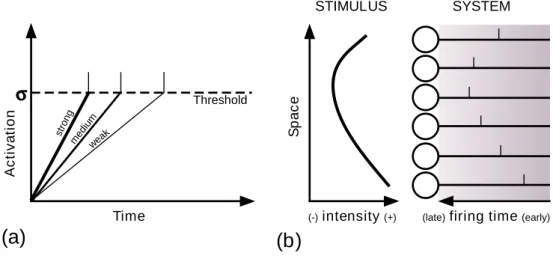
Figure 1.7: Intensity-to-latency conversion. (a) For a single neuron, the
weaker the stimulus, the longer the time-to-first-spike. (b) When presented to a population of neurons, the stimulus evokes a spike wave, within which asynchrony encodes the information (reproduced with permission from Guy-onneau et al. (2004))
strated that STDP increased the postynaptic spike time precision by selecting inputs with low time jitter.
Guyonneau et al. (2005) tested the robustness of Song et al. (2000)’s re-sults in more challenging conditions, including spontaneous activity or jitter. Furthermore they also demonstrated that neither firing rate or even syn-chrony are relevant in the STDP selection process: only the latency matters. STDP was also applied in visual cortex models with asynchronous spike propagation. Those models assumed one spike per neuron only (see Sec-tion 1.6.2), and an intensity-to-latency conversion in the first layer (see Fig. 1.7).
Delorme et al. (2001) and Guyonneau (2006) both showed that V1 simple cells’ Gabor style orientation selectivity could emerge by applying STDP on spike trains coming from LGN ON- and OFF-center cells modeled as Difference-of-Gaussian (DoG) filters.
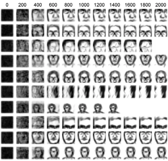
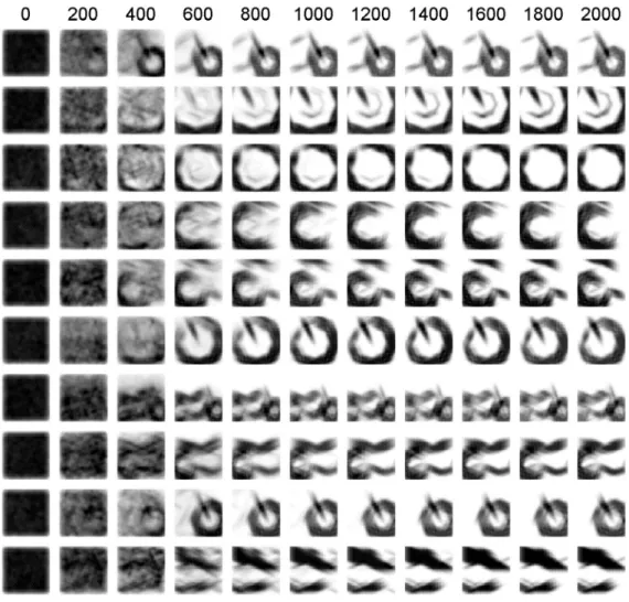
Guyonneau et al. (2004) used Gabor filters as inputs and propagated the same image repeatedly. The earliest spikes thus corresponded to the most salient edges of the image. By concentrating weights on the corresponding synapses STDP led to an interesting visual form detector, as can be seen on Fig. 1.8. Note that this study differs from the one presented in Chapter 2 in
that it is holistic and not feature-based.
1.8
Original contributions
1.8.1
STDP-based visual feature learning
In this study I essentially put together three ideas in the literature:
1. Multi-layer hierarchical models for robust feature-based object recog-nition, exemplified by (Fukushima, 1980; LeCun and Bengio, 1998; Riesenhuber and Poggio, 1999; Wallis and Rolls, 1997; Rolls and Mil-ward, 2000; Stringer and Rolls, 2000; Serre et al., 2007) (but none of these models learns in a biologically plausible manner)
2. Time-to-first spike coding. In the first layers of the network the more strongly a cell is activated the earlier it fires a spike as in (VanRullen et al., 1998; VanRullen and Thorpe, 2001).
3. STDP. Neurons at later stages of the system implement STDP, which had been shown to have the effect of concentrating the synaptic weights on afferents that systematically fire early, which causes the postsynaptic spike latency to decrease (Song et al., 2000; Gerstner and Kistler, 2002; Guyonneau et al., 2005).
I demonstrated that when such a hierarchical system is repeatedly pre-sented with natural images, the intermediate level neurons equipped with STDP naturally become selective to patterns that are reliably present in the input, while their latencies decrease, leading to both fast and informative responses. This process occurs in an entirely unsupervised way, but I then showed that these intermediate features are able to support robust catego-rization.
The resulting model is appealing because it has some of the properties of other hierarchical models (robust object recognition without combinato-rial explosion), but can recognize objects quickly, as has been suggested in experimental literature.
This study has been published:
Masquelier T, Thorpe SJ (2007) Unsupervised learning of visual features through spike timing dependent plasticity. PLoS Comput Biol 3(2): e31. doi:10.1371/journal.pcbi.0030031
0 0.5 1 500 1000 σ 100 0 σ 50 0 0.5 1 0 0.5 1 0 0.5 1 0 σ 0 σ 10 0 σ 1
Receptive field Post-synaptic
potential Synaptic Weights
0 100 200
Time (ms) Rank
(1250 earliest activated inputs) Learning
step
(linear reconstruction)
Figure 1.8: Einstein: STDP learning of a V1-filtered face. A population of V1-like cells encodes an orientation for each pixel in the image presented to the network (here, Einstein’s face); each cell acts as an intensity-to-latency converter where the latency of its first spike depends on the strength of the orientation in its receptive field. Time taken to achieve recognition of the stimulus decreases (middle column) while a structured representation emerges and stabilizes (left column) that is built upon the earliest afferents of the input spike wave (right column). Note that the information concerning the evolution of the synaptic weights in the course of learning is represented twice on this figure. First in the distribution of synaptic weights on the right. It is also present in the receptive field on the left, that is linearly reconstructed based on the synaptic weights and the selectivity of the corresponding afferent neurons (here, orientation selective filters). Reproduced with permission from Guyonneau et al. (2004)
face feature learning were also presented in the conference NeuroComp 2006, Pont-à-Mousson, France (see Section B.2 for the conference paper and poster).
1.8.2
STDP-based spike pattern learning
The main limitation in the above-mentioned work on STDP-based visual feature learning – as well as in many STDP studies (Song et al., 2000; Delorme et al., 2001; Guyonneau et al., 2005; Gerstner et al., 1996) – is the assumption that the input spikes arrive in discrete volleys, each one corresponding to the presentation of one stimulus (or the maximum of a brain oscillation). The stimulus onset (or the maximum of the oscillation) is then an explicit time reference that allows defining a time-to-first spike (or latency) for each neuron. What happens in a more continuous world was unclear.
This is the reason why I started a second study, presented in Chapter 3, not restricted to vision, where one receiving STDP neuron integrates spikes from a continuously firing neuron population. It turns out, somewhat sur-prisingly, that STDP is able to find and track back through spatio-temporal spike patterns, even when embedded in equally dense ‘distractor’ spike trains – a computationally difficult problem.
STDP thus enables some form of temporal coding, even in the absence of an explicit time reference. This means that global discontinuities such as saccades or micro-saccades in vision and sniffs in olfaction, or brain oscilla-tions in general are not necessary for STDP-based learning. Given that the mechanism exposed here is simple and cheap it is hard to believe that the brain did not evolve to use it.
This second study has also been published:
Masquelier T, Guyonneau R, Thorpe SJ (2008) Spike Timing Dependent Plasticity Finds the Start of Repeating Patterns in Continuous Spike Trains. PLoS ONE 3(1): e1377. doi:10.1371/journal.pone.0001377
The original paper can be found on Section A.2.
1.8.3
Visual learning experiment
One of the predictions of the two STDP models of Chapters 2 and 3 is that visual responses’ latencies should decrease after repeated presentations of a same stimulus. In Chapter 4 I tested this prediction experimentally by inferring the visual processing times through behavioral measures.
In a previous study Fabre-Thorpe et al. (2001) looked for an eventual experience-induced speed-up effect, using the animal/non-animal manual