HAL Id: hal-02099906
https://hal.laas.fr/hal-02099906
Submitted on 15 Apr 2019
HAL is a multi-disciplinary open access
archive for the deposit and dissemination of
sci-entific research documents, whether they are
pub-lished or not. The documents may come from
teaching and research institutions in France or
abroad, or from public or private research centers.
L’archive ouverte pluridisciplinaire HAL, est
destinée au dépôt et à la diffusion de documents
scientifiques de niveau recherche, publiés ou non,
émanant des établissements d’enseignement et de
recherche français ou étrangers, des laboratoires
publics ou privés.
Optimised dynamic temperature operating mode
specifically dedicated to micromachined SnO2 gas
sensors
Frédéric Parret, Philippe Menini, A. Martinez, K. Soulantika, A. Maisonnat,
Bruno Chaudret
To cite this version:
Frédéric Parret, Philippe Menini, A. Martinez, K. Soulantika, A. Maisonnat, et al.. Optimised dynamic
temperature operating mode specifically dedicated to micromachined SnO2 gas sensors. 19th European
Conference on Solid-State Transducers (EUROSENSORS XIX), Sep 2005, Barcelona, Spain.
�hal-02099906�
OPTIMISED DYNAMIC TEMPERATURE OPERATING MODE
SPECIFICALLY DEDICATED TO MICROMACHINED SnO
2GAS SENSORS**
F. Parret
1*, P. Menini
1, A. Martinez
1, K. Soulantica
2, A. Maisonnat
2, B. Chaudret
21 Laboratoire d’Analyse et d’Architecture de Systèmes (CNRS-LAAS), *
E-mail : [email protected] http://www.laas.fr 7 Avenue du Colonel Roche, 31077 Toulouse-France.
2
Laboratoire de Chimie de Coordination (CNRS-LCC), 205 route de Narbonne, 31077 Toulouse cedex 4, France.
** Presently developed in the context of “NANOSENSOFLEX” project and funded by European Commission (GROWTH-G5RD-CT-2002-00722)
Abstract: In this paper, we show the influence of short temperature variations on the transient response of a
SnO2 nanoparticular gas sensor. By consideration of the shape and time constants of the normalized response
curves, we can differentiate different gasses mixtures at a ppm level. This new method of analysis is promising to conceive a gas detector based on combination of temperature profiles and different sensitive layers.
Keywords: Micromachined gas sensor; Temperature cycling; Discriminant variables
INTRODUCTION
Previous studies on the development of gas sensors based on metal-oxides have been designed with for objective to reduce dimensions of these gas sensors. Currently, with the combination of nanotechnology and microelectronic processes, it can be possible to reduce the power consumption with low cost. Previous studies have demonstrated the interest to use this gas sensor in temperature modulation [1] improving these performances in term of selectivity and sensitivity for gasses discrimination [2] and also to reduce the influence of relative humidity [3]. These features allow extracting more useful information of the sensing processes to be used in gas identification and quantification via mathematical techniques of classification and analysis [4].
In the frame of the “Nanosensoflex” project, this type of gas sensors has been developed, formed by a microhotplate platform [5] and a nanoparticular SnO2 sensing layer [6] with or without doping agent
[7].
This article deals with a nanoparticular SnO2 gas
sensor associated to an optimised temperature profile applied on heating resistor in the goal to observe the shape of the sensor transient responses depending of the surrounding atmosphere.
SENSOR DESCRIPTION
The sensor used in this study is formed by a microhotplate platform and a nanoparticular SnO2
sensing layer. The microhotplate architecture (Fig. 1) was initially developed by Motorola and presently exploited by Microchemical Sensors S.A. A SiOxNy membrane of 2 m of thickness supports
a polysilicon heater of 600m x 430m. Dimensions have been optimised to achieve good thermo-mechanical reliability and good homogeneity of temperature on the active area.
The heater can reach temperatures of about 500oC with power consumption lower than 100mW. The metal-oxide used in this sensor is a crystalline SnO2 nanomaterial synthesized by the
decomposition and oxidation of a tin based organometallic precursor ([Sn(NMe2)2]2), the mean
grain size obtained is 15 nm of diameter.
Fig. 1. Top view of a SnO2 gas sensor
This material is then deposited using a microinjector technique over the two electrodes placed in the homogeneous temperature region of the heater. This heater permits the full oxidation into SnO2 with a controlled temperature cycle from
ambiant to 500°C.
EXPERIMENTAL RESULTS
The experimental set-up consists of a gas delivery system, an exposure glass vessel and an electronic circuit for resistance determination through voltage measurements. Tests have been performed under 3 gasses (CO, NO2 and C3H8) and mixtures of
these gasses (with concentrations of 200, 1.8 and 150 ppm respectively). The relative humidity is fixed at 50% for a constant flow rate of 500 ml/min.
Fig. 2. An example of test profile applied on heater
We have designed different test profiles of temperature applied on heater. These tests are made up of various flexible parameters like temperature offset, temperature variations (noted dT) and period (Fig 2).
In first time, an optimisation on the period has been studied to eliminate the resistance drift over time of the sensitive layer. In order to observe the transient behaviour of sensing layer, the period must be higher at 0.5 second. Then, to eliminate the resistance drift until this isotherm value, the period does not exceed 5 second.
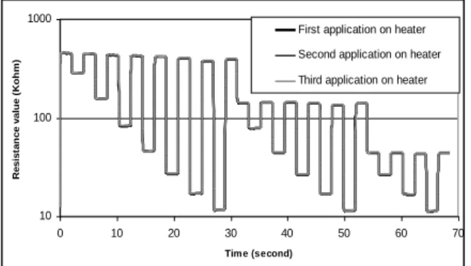
Fig. 3. Undoped sensor response: 3 sequences referenced at the same time.
Typical response curves of the pulsed sensor when exposed to CO (200 ppm) are shown on figure 3. These curves have been obtained reproducibly. Effectively, it can be observed that to a given temperature value always corresponds similar resistance values when the temperature profile is applied at 3 different times.
10 100 1000 0 10 20 30 40 50 60 70 Time (second) R e s is ta nc e v a lue ( K oh m ) Profile 1 Profile 2
Fig. 4. CO response of an undoped sensor for two different profile.
This reproducibility is also reveals by the figure 4 which shows the sensing layer resistance behavior under 200 ppm of CO, for two different profiles. It can be seen that resistance values, at a given temperature level, are identicals independently of the shape of the temperature profile.
Fig. 5. Undoped sensor resistance response under gas.
Finally, it can be seen on figure 5, reduction and oxidation reactions of the resistance of an undoped sensor, identicals like isotherm behaviour, when this one is exposed to reductor gasses like CO and C3H8 and oxidant gasses like NO2.
In order to get a more accurate insight on the transient responses of the sensitive layer on each temperature variation, each resistance value Ri is
normalized according to the following equation:
f f i
n R R R
R ( )/ (1) Where Rn is the normalized value for the resistance
Ri measured at t and Rf is the last value measured
on each step of temperature.
We observed that the shape of the response curve Rn(t), for a given temperature variation, depends of
the surrounding atmosphere.
Fig. 6. Normalized transient response curves from 300 to 400°C.
Typical normalized response curves of an undoped sensor can be observed on figure 6. The shape of this response curve (peak position and slope of the quasi linear part) is considerably affected by exposed gasses (i.e. CO, 200 ppm or C3H8, 150
ppm, or NO2, 1.8 ppm or mixtures of these gasses).
With the same gas sensor but on a different temperature variation, an other shape of the transient response can be observed on figure 7
-0.15 -0.1 -0.05 0 0.05 0.1 0.15 0.2 0 0.5 1 1.5 2 Time (second) Rn w ithou t unit {1} {7} {6} {8} {2}, {5} overlap {3} {4} {1} Air {2} CO {3} C3H8 {4} NO2 {5} CO-C3H8 {6} CO-NO2 {7} CO-NO2-C3H8 {8} NO2-C3H8 -0.15 -0.1 -0.05 0 0.05 0.1 0.15 0.2 0 0.5 1 1.5 2 Time (second) Rn w ithou t unit {1} {7} {6} {8} {2}, {5} overlap {3} {4} {1} Air {2} CO {3} C3H8 {4} NO2 {5} CO-C3H8 {6} CO-NO2 {7} CO-NO2-C3H8 {8} NO2-C3H8 10 100 1000 10000 100000 0 10 20 30 40 50 60 70 Time (second) R es ist an c e va lu e (K o h m ) {1} Air, {2} 200ppm CO, {3} 150ppm C3H8, {4} 1.8ppm NO2 {2} {3} {4} {1} 10 100 1000 10000 100000 0 10 20 30 40 50 60 70 Time (second) R es ist an c e va lu e (K o h m ) {1} Air, {2} 200ppm CO, {3} 150ppm C3H8, {4} 1.8ppm NO2 {2} {3} {4} {1} 10 100 1000 0 10 20 30 40 50 60 70 Tim e (second) Re s is ta n c e v a lu e ( Ko h m )
First application on heater Second application on heater Third application on heater 0 100 200 300 400 500 600 0 10 20 30 40 50 60 Tim e (second) T e m p e ra tu re ( °C) Temperature offset Period of signal Temperature variation (dT) 0 100 200 300 400 500 600 0 10 20 30 40 50 60 Tim e (second) T e m p e ra tu re ( °C) Temperature offset Period of signal Temperature variation (dT)
which is pronounced when NO2 (or mixture of NO2)
are exposed on the gas sensor.
Fig. 7. Normalized transient response curves from 110 to 240°C .
When the temperature increases, the shape of the normalized resistance variations can be sum up with the curves of previous figures. Typical response curves of an undoped gas sensor can be defined with negative slope and a long time constant (170 ms about) when NO2 (or mixture with
NO2) are exposed on the sensor for low
temperature variations. For the other gasses, CO and C3H8 gasses, the behavior is quasi the same
than under synthetic air.
In order to modify the shape of the response curves, at the time of CO and C3H8 gasses
exposition, the operating temperature level must be higher. From 250°C until the allowed maximum temperature (about 500°C), the influence of NO2 is
less pronounced. Then, CO and C3H8 gasses
exposition creates peaks or the combination of peaks and slopes for the gasses mixture. The discrimination of these gasses can be realize with the time of peak position corresponding at 54 and 63 ms respectively for CO and C3H8 gasses.
Moeover, the temperature offsets induce few influences on the shapes.
It’s also very interesting to observe the response curves when temperature level goes down.
In order to compare transient response curves when temperature level goes down and up, we have inverse the normalization with the following relation: f i f n R R R R ( )/ (2)
Where Rn is the normalized value for the resistance
Ri measured at t and Rf is the last value measured
on each step of temperature.
It can be seen three phenomena according to temperature level.
In first time, with low operating temperature, the response of an undoped sensor is more affected when this one is exposed to NO2 gas and mixture
with NO2 (Fig. 8).
Fig. 7. Normalized transient response curves from 440 to 60°C.
Next, with a temperature upper to 250°C, the shape under NO2 gas and mixture with NO2 is fully
changed with simple slopes. Moreover, the sensor response under CO becomes different from synthetic air and C3H8 (Fig. 9).
Fig. 8. Normalized transient response curves from 440 to 200°C.
Finally, with a temperature upper to 380°C, it can be observed on the figure 9, the discrimination between C3H8 and synthetic air that constitutes a
good result.
Fig. 9. Normalized transient response curves from 440 to 350°C.
These results demonstrate the interest to observe the shape of the normalized sensing layer response which depends of the temperature variations and, especially, affected via the surrounding atmosphere.
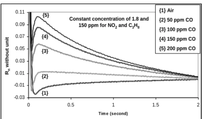
Moreover, it can be possible to discrimine, with the shape analysis by consideration of peak values and time constants, the concentration of one gas in a mixture. In example, with the figure 10, we can
-0.15 -0.1 -0.05 0 0.05 0.1 0 0.5 1 1.5 2 Tim e (second) {1} Air {2} CO {3} C3H8 {4} NO2 {5} CO-C3H8 {6} CO-NO2 {7} CO-NO2-C3H8 {8} NO2-C3H8 Rn w it h o u t u n it {1} {3} {2}, {5} overlap {8} {7} {4} {6} -0.15 -0.1 -0.05 0 0.05 0.1 0 0.5 1 1.5 2 Tim e (second) {1} Air {2} CO {3} C3H8 {4} NO2 {5} CO-C3H8 {6} CO-NO2 {7} CO-NO2-C3H8 {8} NO2-C3H8 Rn w it h o u t u n it {1} {3} {2}, {5} overlap {8} {7} {4} {6} -0.1 -0.05 0 0.05 0.1 0.15 0 0.5 1 1.5 2 Time (second) {1} Air {2} CO {3} C3H8 {4} NO2 {5} CO-C3H8 {6} CO-NO2 {7} CO-NO2-C3H8 {8} NO2-C3H8 Rn w it h o u t u n it {1}, {3} overlap {2}, {5} overlap {4} {7} {8} {6} -0.1 -0.05 0 0.05 0.1 0.15 0 0.5 1 1.5 2 Time (second) {1} Air {2} CO {3} C3H8 {4} NO2 {5} CO-C3H8 {6} CO-NO2 {7} CO-NO2-C3H8 {8} NO2-C3H8 Rn w it h o u t u n it {1}, {3} overlap {2}, {5} overlap {4} {7} {8} {6} -0.15 -0.11 -0.07 -0.03 0.01 0.05 0 0.2 0.4 0.6 0.8 1 1.2 1.4 1.6 1.8 2 Time (second) {1} Air {2} CO {3} C3H8 {4} NO2 {5} CO-C3H8 {6} CO-NO2 {7} CO-NO2-C3H8 {8} NO2-C3H8 Rn w it h o u t u n it {1} {2}, {3} and {5} overlap {4} {8} {6} {7} -0.15 -0.11 -0.07 -0.03 0.01 0.05 0 0.2 0.4 0.6 0.8 1 1.2 1.4 1.6 1.8 2 Time (second) {1} Air {2} CO {3} C3H8 {4} NO2 {5} CO-C3H8 {6} CO-NO2 {7} CO-NO2-C3H8 {8} NO2-C3H8 Rn w it h o u t u n it {1} {2}, {3} and {5} overlap {4} {8} {6} {7} -0.2 -0.1 0 0.1 0.2 0 0.5 1 1.5 2 Time (second) Rn w ithou t unit {1} {2}, {5} overlap {3} {4} {8} {6} {7} {1} Air {2} CO {3} C3H8 {4} NO2 {5} CO-C3H8 {6} CO-NO2 {7} CO-NO2-C3H8 {8} NO2-C3H8 -0.2 -0.1 0 0.1 0.2 0 0.5 1 1.5 2 Time (second) Rn w ithou t unit {1} {2}, {5} overlap {3} {4} {8} {6} {7} {1} Air {2} CO {3} C3H8 {4} NO2 {5} CO-C3H8 {6} CO-NO2 {7} CO-NO2-C3H8 {8} NO2-C3H8
observe the sensor response under the mixture of CO, C3H8 and NO2, where CO-concentration
increases.
Fig. 10. Normalized transient response curves from 350 to 520°C.
DISCUSSION
Figures 6 and 7 show the normalized variation of resistance against time for injection of various resistive and oxidative gas mixtures upon increasing the temperature whereas figures 8-10 display the same phenomena but upon decreasing the temperature. These curves bring to our attention several interesting points :
- at low temperature the resistive gas CO and C3H8
do not play a role in the resistance modification (figure 8); this can be easily interpreted in terms of absence of reaction between CO or propane on one side and O2 on the other catalysed by the
SnO2 sensitive layer;
- at higher temperature (figure 9), the barrier of activation of the oxidation reaction of CO is low enough for the reaction to proceed whereas that for C3H8 is higher; it is therefore possible to
discriminate one from the other;
- at even higher temperature (figure 10) both CO and C3H8 are oxidized and they are more difficult to
distinguish; only the peak position reveals the different nature of the gasses
- there is a somewhat similar phenomenon for oxidizing gasses but reverse. Thus, at low temperature (figure 7) NO2 displays an oxidizing
power larger than air and is therefore detected by a transient peak; this peak tends to disappear at higher temperature where the oxidation rate of the sensitive layer is fast enough
- the mixture of NO2 and a reducing gas only
reveals NO2 at low temperature whereas the
opposite effects are clearly seen at 350°C (figure 10).
These data demonstrate the complexity of catalytic reactions at the surface of the tin oxide layer and associated to the gas detection. This is clearly revealed by the transient peaks which are associated with difference in kinetics of the various reactions involved. This can be associated with the thermodynamic characterization of the reactions associated with the final resistance measured when exposing a sensitive layer to a define gas and can
lead to a finger print of various gasses and gas mixtures.
CONCLUSION
A new generation of gas sensors based on nanoparticular SnO2 sensitive layer has been
elaborated. We have developed and optimised a test profile of temperature to find the best variation competent to get reproducible information for the gas detection. First results show that the shape of the sensing layer response on a temperature variation is significantly affected by a gas or gasses mixture. These shapes, formed with peak and slope, can be treated and exploited. These results are promising and a study is in progress for the realisation of a gas detection prototype based on the shape analysis and the time constants with an optimise temperature profile.
REFERENCES
1. T. Viard, PhD Thesis; LAAS report, No. 99554, 1999.
2. M. Schweizer-Berberich, et al. Sensors and Actuactors, B65 (2000), pp 91-93.
3. M. Guerrero, “Method of C2H4 detection in
humid atmospheres using nanoparticular SnO2 gas sensor”, Eurosensors XVII, pp
873-875, sept 2003
4. M.Baumbach, et al. 12th International Trade Fair of Sensorics, in press, 10-12 May, 2005.
5. S. Astie, PhD Thesis ; LAAS report, No 98537, 1998.
6. P. Fau, et al., European patent n°98400246.9-2104.
7. Maisonat, et al. Proceeding Eurosensors XVIII, Rome, Italy, Sep. 12-15, 2004.
-0.03 -0.01 0.01 0.03 0.05 0.07 0.09 0.11 0 0.5 1 1.5 2 Tim e (second) {1} Air {2} 50 ppm CO {3} 100 ppm CO {4} 150 ppm CO {5} 200 ppm CO Rn w it h o u t u n it {1} {2} {3} {4} {5}
Constant concentration of 1.8 and
150 ppm for NO2and C3H8 -0.03 -0.01 0.01 0.03 0.05 0.07 0.09 0.11 0 0.5 1 1.5 2 Tim e (second) {1} Air {2} 50 ppm CO {3} 100 ppm CO {4} 150 ppm CO {5} 200 ppm CO Rn w it h o u t u n it {1} {2} {3} {4} {5}
Constant concentration of 1.8 and