HAL Id: hal-02017296
https://hal-ifp.archives-ouvertes.fr/hal-02017296
Submitted on 13 Feb 2019HAL is a multi-disciplinary open access archive for the deposit and dissemination of sci-entific research documents, whether they are pub-lished or not. The documents may come from teaching and research institutions in France or abroad, or from public or private research centers.
L’archive ouverte pluridisciplinaire HAL, est destinée au dépôt et à la diffusion de documents scientifiques de niveau recherche, publiés ou non, émanant des établissements d’enseignement et de recherche français ou étrangers, des laboratoires publics ou privés.
Approach
N. Henn, Michel Quintard, B. Bourbiaux, S. Sakthikumar
To cite this version:
N. Henn, Michel Quintard, B. Bourbiaux, S. Sakthikumar. Modelling of Conductive Faults with a Multiscale Approach. Oil & Gas Science and Technology - Revue d’IFP Energies nouvelles, Institut Français du Pétrole, 2004, 59 (2), pp.197-214. �10.2516/ogst:2004015�. �hal-02017296�
Modelling of Conductive Faults
with a Multiscale Approach
N. Henn
1, M. Quintard
2, B. Bourbiaux
3and S. Sakthikumar
41 Gaz de France, Direction Exploration-Production, 361, avenue du Président-Wilson, BP 33, 93211 La Plaine-Saint-Denis - France 2 Institut de mécanique des fluides, (IMFT), allée Professeur Camille-Soula, 31400 Toulouse - France
3 Institut français du pétrole, Direction Gisements, 1 et 4, avenue de Bois-Préau, 92852 Rueil-Malmaison Cedex - France 4 Total, Exploration-Production, 2, place Coupole, 92400 Courbevoie - France
e-mail: [email protected] - [email protected] - [email protected] - [email protected]
Résumé — Modélisation des failles conductrices. Approche multiéchelle — La plupart des gisements
pétroliers sont traversés par des fractures de multiples échelles. Parmi celles-ci, les failles conductrices peuvent avoir un rôle majeur sur les performances de production. Leur modélisation est problématique sur deux points :
– la nécessité d’une représentation explicite des failles avec des dimensions de maille faibles ; – la modélisation des échanges polyphasiques entre le milieu faille et le milieu encaissant.
Dans cet article, nous proposons un modèle performant d’un point de vue représentativité physique et coût numérique pour incorporer des failles conductrices dans des simulateurs simple ou double milieu. Pour valider notre approche et démontrer son efficacité, nous présentons les résultats de simulations d’écoulements polyphasiques dans des secteurs représentatifs de gisements.
Abstract — Modelling of Conductive Faults with a Multiscale Approach — Some of the most productive oil and gas reservoirs are found in formations crossed by multiscale fractures/faults. Among them, conductive faults may closely control reservoir performance. However, their modelling encounters numerical and physical difficulties linked with:
– the necessity to keep an explicit representation of faults through small-size gridblocks; – the modelling of multiphase flow exchanges between the fault and the neighbouring medium.
In the present work, a physically representative and numerically efficient modelling approach is proposed to incorporate subvertical conductive faults in single- and dual-porosity simulators. To validate our approach and demonstrate its efficiency, simulation results of multiphase displacements in representative field sector models are presented.
SYMBOLS
adim Dimensionless number kr Relative permeability Pc Capillary pressure, Pa G VE dimensionless number K Permeability, m2 K* Equivalent permeability, m3 L Length, m δx Length, m V Filtration velocity, m·s–1 µ Dynamic viscosity, Pa·s–1
P Pressure, Pa ρ Density, kg·m–3 g Gravity acceleration, m·s–2 z Vertical coordinate x Horizontal coordinate y Horizontal coordinate S Saturation T Transmissivity, m3 e Thickness, m t Time, s Φ Potential, Pa
GOR Production gas-oil ratio, cft/bbl N Number of gridblocks
I Index of gridblock
∆ Difference operator. Subscripts
p Phase
top Top of fault gridblock bot Bottom of a fault gridblock op Contact between oil and p-phase c Center of a fault gridblock
f Fissure
h Harmonic mean
Pc0 Zero capillary pressure
m Matrix
s Single medium n Neighbouring medium
F Fault
F* Fault subgridblock
X Horizontal direction orthogonal to the fault plane Y Fault plane direction
Z Vertical direction r Residual saturation i Irreducible saturation w Water o Oil g Gas. INTRODUCTION
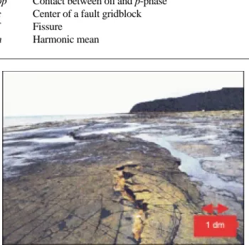
Naturally fractured petroleum reservoirs pose a real challenge to engineers. The description of the fractures, combined with the knowledge of the physics of multiphase flow in fractured porous media and numerical modelling, provide the basis for understanding and forecasting the performance of these reservoirs. Most naturally fractured reservoirs include fractures with multiple length-scales. The scale of small-scale fractures (Fig. 1), called fissures, is centimetric to decametric. This characteristic size is smaller than the typical gridblock size of reservoir models, which is about one hundred meters. At the reservoir scale, a network of conductive faults may also exists. These faults are less dense than the fissures, but, most often, cross the entire thickness of the reservoir and extend over several kilometers (Fig. 2).
The main characteristic of fissured reservoirs is the presence of two contrasted media: the fissure and the matrix. The fluid transport is located within the fissure network. The fissures bypass the neighbouring matrix blocks that contain the oil.
Figure 1 Fissure network.
Figure 2 Fault network.
Faults often appear as high fracture density linaments concentrating tectonic movements. Regarding fluid transport, they have different roles. As regards transverse flows, faults can be either permeable or impermeable depending on fault plane cementation (Fig. 3). Sealing faults are responsible for altering reservoir continuity. Concerning flows along fault planes, favorable geomechanical conditions may lead faults to behave as very conductive flowpaths.
While fluids are flowing rapidly within the faults, they can exchange fluids with the neighbouring formations. The impact of conductive faults on oil recovery can be either positive or negative. Trocchio (1989) presents a reservoir study in which production wells located near conductive faults are characterized by early water breakthroughs and a rapid increase of water-cut, whereas Gilman et al. (1994) shows that the productivity index of horizontal wells increases significantly when they are crossed by conductive faults. This paper focuses on the modelling of multiphase flows in reservoirs crossed by conductive faults. First, it reviews the usual methods for this modelling in conventional reservoir simulators. Whatever the method, it entails draw-backs regarding both the geometrical description of conductive faults, the multiphase fluid flows within the faults, and the numerical performance of the models. The new conductive fault model proposed in this paper has been introduced into a conventional three-phase reservoir simulator based on a black-oil thermodynamic model, a fully-implicit numerical scheme and Cartesian grids. Mass balance equations are discretized by the finite-volume method (Gallouët et al., 1994). This paper presents the physical basis of our approach, that is the vertical equilibrium (VE) concept used to model fluid flows within faults, and the coupling between the VE fault model and single- or dual-medium representation of the reservoir. Finally, to validate our approach and demonstrate its efficiency, simulation results of multiphase displacements in representative field sector models are presented as well as the history matching
of a production well located in a faulted sector of a North-African oil field.
1 FRACTURED RESERVOIR MODELLING -BACKGROUND
1.1 Fissured Reservoir Modelling
As a fissure network is extremely complex, a detailed gridding of such a network is practically impossible (Fig. 4). To overcome this problem, simplified models have been developed. In most conventional reservoir simulators, flows in a fissured reservoir can be modelled by using the dual-medium concept introduced by Barenblatt and Zheltov (1960). In this approach, the fissured medium is described by two equivalent media corresponding to the fissures and the matrix blocks. The fluid transfer between the fissure medium and the matrix medium is expressed with the help of a constant exchange term called the shape factor. In fissured reservoir engineering, there is a permanent interest in the expression of the shape factor.
Warren and Root (1963) presented an analytical solution for interpreting well tests in naturally fissured reservoirs. To get an expression of the shape factor, their work assumed a continuous system of orthogonal fissures (Fig. 5). Super-imposed on this system, a set of identical rectangular parallelepipeds represents the matrix blocks.
By using fine gridded fissured media, Granet (2000) com-puted reference solutions for matrix-fissures transfers and evaluated the reliability of expressions for the shape factor proposed by different authors. For slightly compressible one-phase flow, she showed that the one obtained theoretically by Quintard and Whitaker (1996) gives the best match com-pared to her reference model. A discussion on the use of dual-media models and the choice of shape factors is beyond the scope of this paper. A detailed and comparative analysis
X-permeable fault Z X Z X Surrounding formation
X-impermeable fault Y-conductive fault
Y F A U L T Figure 3
of all the proposed shape factors can be found in Landereau et al. (2001).
Unfortunately, no theoretical expression of the shape factor has been found for multiphase flows. It is largely admitted that it depends on the transfer mechanisms. In most reservoir simulators, the used shape factor for multiphase flows is the one proposed by Kazemi (1976).
Fissured media can also be modelled by a single-medium model, see for instance the homogenization results by Lee et al. (1999). It consists in considering equivalent permeabilities in a single-medium model, which take into account both the fissure and matrix media. Although it is sometimes preferred to dual-medium models because of less input data and a lower numerical cost of the simulations, a single-medium model leads to imprecise predictions. In any case, such a model has also been considered in the numerical model presented in this paper.
1.2 Modelling of Reservoirs Crossed by Conductive Faults
There exist several methods described in the oil and gas literature for modelling of conductive faults in a reservoir. The most straightforward method is to use very narrow gridblocks to model both the fault and the vicinity of the fault. This method leads to a good physical representation of the fault zone but unacceptable run time due to the numerical resolution (Hearn et al., 1997).
A more flexible approach is to model the faults as part of the fissure grid system of a dual-medium model (Gilman et al.,1994). Nevertheless, this method is not convenient since it cannot dissociate the roles of fissures and faults in multiscale fractured reservoirs.
Conductive faults could be modelled by normal-size gridblocks that are assumed to contain embedded fault zones (Trocchio, 1989). The fault gridblocks are assigned equiv-alent permeabilities to simulate the fluid flow in the faults. This method entails three drawbacks:
– building such a model is time-consuming for a complex network;
– it overestimates breakthrough times;
– coarse grids do not allow to simulate development sce-narios with a close well spacing in densely-faulted zones. To model conductive faults, Lee et al. (1999) proposed the well-like approach used in conventional reservoir simulators. They introduce a transport index, similar to the productivity index in well modelling, to formulate the fluid exchanges between the fault and the gridblock enclosing the fault. As the well-like equations imply no accumulation terms, this approach does not model the volume and the distribution of fluids within faults and cannot predict the gravity exchange between the fault and the neighbouring medium. Moreover, like the previous method, this approach is not adapted for the simulation of infill drilling scenarios in densely-faulted regions.
More recently, a novel numerical technique, based on domain decomposition, was implemented to predict fluid migration along faults during the geological history of hydro-carbon-bearing sedimentary basins (Schneider et al., 2002). 1.3 Conclusion
In our model, fissures can be modelled either by the dual-medium approach or by using a single-dual-medium represen-tation of the reservoir. The Warren and Root model (Fig. 5) is used to express the fluid transfer between the fissure and the matrix media (Quandalle and Sabathier, 1987). Regarding conductive fault modelling, the analysis of the usual methods led us to conclude that a specific model of conductive faults is needed with a precise and flexible description of fault geometry and fluid displacements, and with a high numerical performance. Our conductive fault modelling approach is detailed below.
2 CONDUCTIVE FAULT MODELLING
Some authors (Hearn et al., 1997; Gilman et al., 1994) modelled the conductive faults by using explicit gridblocks. This allows to represent precisely the faults paths and to estimate exactly the volume of fluids drained along the faults
Figure 4
Dual-medium approach.
Figure 5
by assigning convenient petrophysical properties in the conductive fault gridblocks. Moreover, this approach permits to know the fluid distribution within a fault and to simulate precisely the fluid transfers between this fault and the surrounding formations. This method is used in our model. Fault gridblocks cross the reservoir over the entire thickness (Fig. 6). Fault gridblock thickness is very small compared to that of conventional reservoir gridblocks (Lm>> LF).
Figure 6
Conductive fault representation.
In addition, we use the VE concept to model fluid flow within the faults. This concept is applicable when viscous forces are negligible compared to gravity and capillary forces. Under the vertical equilibrium assumption, gravity and capillary forces are in equilibrium in the vertical direction. This equilibrium corresponds to a given fluid distribution that can be formulated by simple relations. Thus, conductive faults can be modelled with a unique gridblock in the vertical direction (Fig. 6). Coats et al. (1967) expressed the vertical equilibrium concept in terms of a constant phase potential of a phase p in the portion occupied by this phase along the vertical direction:
(1)
where P is the pressure, ρis the density and g the algebraic value of the gravity acceleration. In this case, the direction of the unit vertical vector points upwards. Martin (1968) proov-ed theoretically these vertical equilibrium equations using the basic flow equations for a compressible three-phase flow.
Several authors attempted to define a validity domain for the vertical equilibrium assumption. Coats et al. (1967) defined two characteristic times corresponding to:
– the vertical flow submitted to gravity and capillary forces; – the horizontal flow.
The ratio of these characteristic times leads to a dimen-sionless number allowing to determine if the vertical equilibrium assumption is valid.
Coats et al. (1971) performed the same work when neglecting capillary forces. Spivak (1974) made the flow equations dimensionless in order to compare the contribution of each force. The dimensionless numbers of Spivak are coherent with those of Coats et al. in the sense that the same parameters favour the vertical equilibrium. They correspond to a high vertical permeability, a low phase horizontal velocity, a large contrast between phase densities, and low phase viscosities. The knowledge of the vertical permeability is very important to validate the use of the VE concept in our model. Unfortunately, this parameter is practically impos-sible to evaluate precisely.
Precise validations require numerical simulations with finely-gridded models in the vertical direction. In the case of a water-oil flow, one can plot the variation of water saturation versus depth for different porous medium/fluid configurations and deduce the limit value of an adequate dimensionless number consistent with the vertical equilibrium. This is illustrated in Figure 7 for several numerical simulations corresponding to the average horizontal flow within a vertical fault. The characteristic dimensionless term for those cal-culations has been chosen following Coats et al. (1971) as: (2) From this example, we see that a value of the criterion, i.e., G, greater than 0.16 ensures that the transition zone is small enough, compared to the fault height.
Figure 7
Validation of VE assumption: saturation versus depth at the mid-position between the injector and the producer.
0 0.2 0.4 0.6 0.8 1.0 1.2 Depth (m) 8100 8120 8140 8160 8180 8200 8220 8240 8260 Water saturation G = 0.04 G = 0.08 G = 0.16 G = 0.4 Inj. Prod. Z Y G K A g Q v w o F o = (ρ –ρ ) µ Φ Φ p p p p P gz z = + ∂ ∂ = ρ 0 F A U L T Lm Throw Z X Neighbouring formation model LF
In our model, given the characteristic length-scales in-volved, we neglect the capillary phenomena in the conduc-tive faults. Consequently, the vertical equilibrium concept implies only gravity forces (Fig. 8). Under these conditions, phases in the fault will be vertically segregated according to their densities.
The horizontal flow of segregated phases along fault planes is formulated with generalized Darcy’s laws using pseudo-functions
(3)
where KYis the longitudinal fault permeability and µthe dynamic viscosity. P is the oil pressure and reference pres-sure. The pseudo-relative permeability and pseudo-capillary pressure are expressed as:
(4)
(5) All vertical positions z are detailed in Figure 8. The pseudo-relative permeability is an average of local relative permeabilities along the vertical direction. Due to the phase segregation, the local relative permeabilities are equal to end-point values. The pseudo-relative permeability is weighted by the absolute horizontal permeability along the vertical direction. It also depends on porosity and saturation
end-points in the fault. The pseudo-capillary pressure is a gravity induced term and has nothing in common with capillary forces.
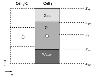
Fluid velocities in a conductive fault can be very high. Our conductive fault model has been developed with a fully-implicit numerical scheme in order to avoid strong numerical constraint on the time step (Aziz and Settari, 1979; Hearn et al., 1997). However, the improved numerical performance of our model mainly results from the decrease of the total number of gridblocks due to the vertical equilibrium assumption. For a full-field model, this numerical gain is low if the number of conductive fault gridblocks is much smaller than the number of conventional reservoir gridblocks in which the vertical equilibrium assumption is not considered. A fault gridblock is generally of a much larger height than neighbouring blocks. Direct coupling between the conductive fault gridblock (F) pressure and saturation and the neigh-bouring gridblock pressures and saturations would be inaccurate. The detailed distribution of fluids within the fault block is required. The local approach consists in discretizing fictitiously the fault gridblock in the vertical direction with respect to the neighbouring medium discretization (Fig. 9).
The segregated state in the fault enables to determine the local values of each phase saturation and pressure in each fault subgridblock (F*):
(6)
If the p-phase is absent in the fault subgridblock, a fictive pressure Pp,F*is defined to enable the calculation of p-phase flow from the neighbouring gridblock (n) to the fault subgridblock (F*). S f S P P Pc g z z p F p F p F F p F p F c F , * , , * , , * ( ) – ( – ) = = + ρ Pcp=
(
ρo–ρp)(
zop–zc)
g kr K z kr S z z K z z p Y p p z z Y z z bot top bot top =(
)
∫ ∫ ( ) ( ) ( ) d d r r r Vp KY kr grad P Pc g p p p p =– ⋅(
( – ) –)
µ ρ (kr Pcp, p): ztop zog zow zbot zc Cell j-1 Cell j Gas Oil Water Z Y Fault gridblock (F) zF* zc Z X Neighbouring medium gridblock (n) Fault subgridblock (F*) Figure 8Gravity equilibrium in a fault gridblock.
Figure 9 Local approach.
3 COUPLING OF A CONDUCTIVE FAULT MODEL AND A SINGLE-MEDIUM MODEL
In this case, the neighbouring medium (n) of the fault is a single medium (s). This single medium could represent either a matrix medium or a homogenized fissured medium. In our model, the mass flow rate of a component k estimated at the interface of two conventional reservoir gridblocks i and j is expressed as:
(7) where T is the transmissivity, Ckpthe mass fraction of the k-component in the p-phase, kr is the relative permeability. The function up(i,j) is equal to i if the phase potential Φpis higher in the gridblock i than in gridblock j and to j in the opposite case. This is commonly known as the upstream numerical scheme (Aziz and Settari, 1979). Its numerical stability makes it the most used numerical scheme in conventional reservoir simulators.
In a black-oil model, the mass fraction of the water component (k = e) in the water phase (p = w) is equal to 1 so that, for the water, the above expression of the mass flow rate becomes:
(8)
The fluid transfers of a p-phase between a fault sub-gridblock (F*) and a neighbouring single-medium sub-gridblock (s) are controlled by a potential difference defined as the difference between the local pressure of the fault sub-gridblock (Fig. 9) and the pressure in the single-medium gridblock:
(9)
expansion capillarity gravity
where PFand Psare the pressures of the reference oil phase. Pcp,s is the capillary pressure of the p-phase in the single-medium gridblock. This expression is composed of three terms corresponding to three exchange mechanisms:
– an expansion term equal to the reference pressure difference;
– a capillary term deriving from the capillary pressure in the matrix;
– a gravity term involving the pseudo-capillary pressure of the fault gridblock.
The fluid transfers between the two media are also controlled by the phase relative permeability.
Hereafter, we analyse the formulation of mass exchanges between a conductive fault and a single-medium reservoir and optimize it in terms of representativity and numerical performance. To this end, we consider two one-dimensional (X) models representing a fault element and the neighbouring single-medium (Fig. 10).
In the reference model, the single medium is finely gridded, the thickness of the single-medium gridblocks being equal to the thickness of the fault. This is a reference model because it reproduces accurately the kinetics of the fluid transfers between the two media. Because of numerical requirements, this model is not usable for reservoir studies. In the coarse model, the single medium is modelled with one gridblock with the horizontal dimension corresponding to that of a conventional reservoir gridblock. Therefore, in the
{
{
{
∆Φp sf, *=Pp F, *–Pp s, =PF –Ps–Pcp s, –Pcp F, + ρpg z( c–zF*) ∆Φp sF, *= Pp F, *–Pp s, Fw ij Tij kr w ij w up i j w ij w ij , , , ( , ) , , = ρ µ ∆Φ Fk ij Tij C kr kp ij p ij p ij p p up i j p ij , , , , , ( , ) , = ∑ ρ µ ∆Φ Single-medium 1 m 1 m 100 m 1D model Fault Coarse model Fault subgridblock Reference model Z X -70 -50 -30 -10 10 30 50 70 90 110 Sw (adim) Swi PC ow (psi) - 1 psi = 6895 Pa 1-Sorw 0.1 0.2 0.3 0.4 0.5 0.6 0.7 0.8 0.9 1 Sw,s,Pc0 Figure 10Study of the local exchange.
Figure 11
X-direction, we get the juxtaposition of a fine, fault sub-gridblock, and a coarse, single-medium gridblock.
At the initial time, the fault subgridblock is filled with an infinite quantity of water whereas the single-medium gridblock(s) is (are) filled with oil and irreducible water (Swi). By capillary imbibition, the water present in the fault flows to the single medium until the capillary equilibrium is reached. As there is no capillary pressure within the fault, this equilibrium is reached when the capillary pressure in the single-medium model is equal to zero. We denoted by Sw,s,Pc0 the equilibrium water saturation, which is equal to 0.4 in our numerical experiments (Fig. 11).
We use the upstream scheme for both models. We plot Figure 12 the variation of the oil recovery in the single-medium model versus time for both models.
We observe that the exchange kinetics is overestimated significantly when using the coarse model. If we refer to the physical problem, the whole flow takes place within the unique single-medium gridblock, which is the downstream gridblock of the water flow. The upstream scheme is not consistent with this flow and this generates the observed overestimation. In this example, when using a two-dimensional model (XZ), we get the same results because capillary forces are preponderant in water-oil flow ex-changes. The upstream scheme is consistent with the coarse model only when water flows from the single medium to the fault medium.
Hereafter, we define a new exchange relative permeability to simulate accurately a water flow from a fault subgridblock to a coarse single-medium gridblock. We consider a coarse one-dimensional model (X-direction) with the notations indicated Figure 13.
We make the assumption that the mean effective multi-phase permeability (K krw) of both gridblocks can be formulated as the harmonic mean of the effective perme-abilities of each gridblock:
(10) where K is the harmonic mean of the absolute permeability:
(11) As δxF* << δxsand KF*≈ Ks, one can deduce from the two previous equations that K≈Ks (Eq. (10)), then krw
≈krw,s (Eq. (11)). The exchange relative permeability krw between the fault and the single-medium is roughly equal to the mean relative permeability of the single-medium gridblock. Consequently, the conventional numerical upstream scheme (Aziz and Settari, 1979) is not consistent when considering fluid flowing from the fault medium to the single-medium. To handle this case, we present hereafter a consistent approach to determine a good estimate of krw.
Figure 12
Oil recovery in the single-medium model.
Figure 13
Coarse model. Notations and water saturation front.
The mean relative permeability of the single-medium gridblock (krw,s) depends on the mean water saturation of this gridblock. The choice of the mean saturation to calculate the mean relative permeability is consistent when calculating an outgoing flow from the gridblock. On the opposite, it is not correct when calculating an incoming flow with no water present in the single-medium gridblock since the relative permeability would be equal to zero. To determine an exchange relative permeability when water flows from the fault to the single-medium requires to focus on the local flow in the single-medium.
When considering a piston-like water displacement in the single-medium, the two-phase flow takes place only in a δx layer of the single-medium gridblock. δx varies with time between 0 and (2*δxs). Within this layer, the water saturation is equal to the capillary equilibrium saturation Sw,s,Pc0if we suppose no capillarity effects within the fault. When consid-ering the δx layer in Equations (8) and (9) instead of δxs, one may deduce the exchange relative permeability as follows:
(12) At short time, this approximation is incorrect because the assumption δxF*<<δx is not valid. Nevertheless, the duration of this period is so short compared to the time
krw s, ≈krw ≈krw s,
(
Sw s Pc, , 0)
Fault subgridblock (F * ) Coarse single-medium gridblock (s) δ xs δ xF* 30 25 20 15 10 5 0 Oil recovery (%) 0.01 0.1 1 10 100 1000 10 000 Time (days) Reference model Coarse model Improved coarse modelδx δx δ δ K x K x K F s F F s s * * * +
(
)
= + δx δx δ δ K kr x K kr x K kr F s w F F w F s s w s * * * , * , +(
)
= +required for the total invasion of the single-medium that we can neglect it.
If the fault subgridblock is partially filled with water, the exchange area used in the mass flow rate expression (Eq. (7)) for the transmissivity T must be a reduced exchange area:
(13) where AsF* is the total exchange area of the fault sub-gridblock. If we take into account the capillary equilibrium relative permeability krw,s(Sw,s,Pc0) and the reduced exchange area in the expression of the water mass flow rate between a fault subgridblock (F*) and a single-medium gridblock (s), we obtain:
(14) We used the above expression to simulate the water flow from the fault to the single medium with the coarse model (Fig. 10) and compared the results with those of both the initial coarse model and the reference model (Fig. 12). We denote the new model as “improved coarse model”. Contrary to the initial coarse model, the exchange kinetics is slightly underestimated when using the improved coarse model. Nevertheless, it gives much better results.
If we consider a gas flow from the fault to the neigh-bouring single medium instead of a water flow, no difference is observed between the coarse model with the upstream scheme and the reference model because of the low gas pressure drops in the single-medium model.
In order to validate the exchange formulation detailed before jointly with our conductive fault model, we now present a water-oil simulation in a sector of a field crossed by a dense network of conductive faults. The sector is a 3D panel edged by two faults (Fig. 14). Thanks to symmetry, the panel behaviour could be modelled on a half-panel edged by one fault (Fig. 15). In this case, there is a water flow along the fault inducing both an early water breakthrough and a rapid increase of the water-cut at a production well located nearby.
The fault conductivity is equal to the longitudinal perme-ability of the fault times its thickness eF, i.e., 15 D.ft (4.86E-12 m3). Regarding the reservoir simulations, our objective is
to get both a good physical representativity and a high numerical performance, i.e., a reliable prediction of the production behaviour at a reasonable numerical cost. Herein, we compare our conductive fault model with finely gridded models. The two main features of the proposed model are: – a one-dimensional segregated flow model representing
conductive faults;
– the specific expression of the water mass flow rate (Eq. (14)) for the exchange between the fault and the neighbouring single-medium.
Figure 14
Structural map of a field crossed by conductive faults.
Figure 15
Description of the conductive fault model.
α = 2.1° 165 ft 500 ft 45 ft 40 ft 35 ft 30 ft 1 ft = 0.3048 m
Conductive fault model
- Segregated flow within fault
- Coarsely-gridded neighbouring single medium (s)
Half-panel Fault Y X Z Y Z X eF = 3 ft Single medium NXs = 4 NYs = 20 NZs = 4 Fault medium NXF = 1 NYF = 20 NZF = 1 Single medium Single medium Fw sF TsF S kr S w sF w sF w F w s w sPc p mF , * * , * , * , * , ( , ) , * = ρ µ 0 ∆Φ AsFred A S sF w F *= ** , *
This latter expression permits to avoid the use of small gridblocks in the vicinity of the fault. Hereafter, the com-parison of the conductive fault model with finely-gridded models allows to determine the contribution of both features.
At the initial time, the single medium is saturated with oil. The fault is assumed to be in connection with an active aquifer. This is reproduced numerically by introducing a fictitious water injector located at the bottom of the structure within the fault (Fig. 17). There is one producer in the single medium panel at the top of the structure. The matrix perme-ability is isotropic and equal to 20 mD (1.97E-14 m2).
Water-oil capillary pressures are only present within the single medium model (Fig. 10). The water-oil relative permeabilities in the single-medium model are nonlinear (Fig. 16).
Figure 16
Water-oil relative permeabilities in the single-medium gridblocks.
In addition to our conductive fault model (Fig. 15), we define two models:
– Model 1 (Fig. 17): both fault and single media are finely-gridded respectively in the vertical direction and in the horizontal direction perpendicular to the fault plane (X). – Model 2 (Fig. 18): it corresponds to model 1 except that
the single medium is coarsely-gridded in the horizontal direction perpendicular to the fault plane.
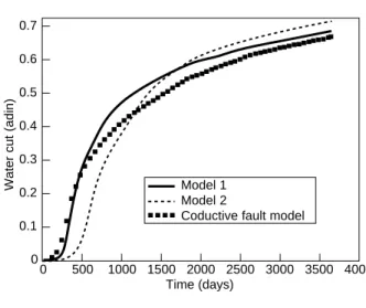
In both models, upstream relative permeabilities are used to compute water flow from the fault to the single medium. Because it is finely-gridded, model 1 is considered as the reference model. The evolution of the production water-cut versus time is plotted in Figure 19 for the three models: – model 1;
– model 2;
– conductive fault model.
The comparison of the three models shows that model 2 predicts a delayed breakthrough time at the production well.
Figure 17
Description of the comparative model 1.
Figure 18
Description of the comparative model 2.
Figure 19 Water-cut at producer. 0.7 0.6 0.5 0.4 0.3 0.1 0.2 0
Water cut (adin)
0 500 1000 1500 2000 2500 3000 3500 4000
Time (days) Model 1 Model 2
Coductive fault model Y X Z Single medium NXmf = 4 NYmf = 20 NZmf = 4 Fault medium NXF = 1 NYF = 20 NZF = 4 Single medium Fault Water injector Water-oil producer Fault path Model 2 Y X Z 10 ft 105 ft 50 ft Single medium NXs = 6 NYs = 20 NZs = 4 Fault medium NXF = 1 NYF = 20 NZF = 4 Single medium Fault Water injector Water-oil producer Model 1 0 0.2 0.4 0.6 0.8 1.0 1.2 0.1 0.2 0.3 0.4 0.5 0.6 0.7 0.8 0.9 1.0 0 krow krw 1-Sorw Swi kr (adim) Sw (adim)
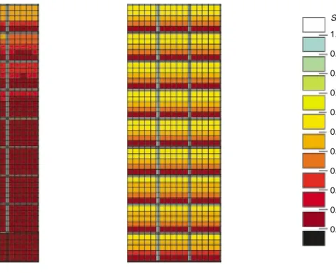
When using both coarse single-medium grid and upstream relative permeabilities, the kinetics of fault-matrix transfers is overestimated. Consequently, water front progression in the fault is slower in model 2 and water reaches the producer later than in model 1 (Fig. 20).
Using our coarsely gridded fault model, we better repro-duce the fault-matrix exchanges, fluid flows within the fault and, finally, we get a better match of the production data (Fig. 21).
Figure 21
Water saturation map. Conductive fault model.
Table 1 compares the numerical and computational per-formances of the three simulations. Linear systems were solved with the conjugate gradient method. We used a SUN Ultra 30 workstation.
Coarse model 2 and our conductive fault model give similar numerical and computational results, with a slight advantage to the conductive fault model. Therefore, the
segregated flow model does not improve dramatically the numerical performance, as compared to coarse gridding of the fault system, especially when the numerical scheme is implicit. On the contrary, the model gives better numerical results than refined model 1 in the sense that it is approxi-mately 4 times faster. Actually, the fine gridblocks present in the vicinity of the fault in model 1 entail time-expensive linear system resolutions.
TABLE 1 Numerical performance
Model 1 Model 2 Conductive fault model Number of gridblocks 560 400 340 Number of time steps 223 207 211 Number of newton iterations 229 210 211 Number of solver iterations 26172 9942 8231 CPU time (s) 252 75 64
Regarding water-oil simulation in a fault panel, we conclude that our model provides improved physical responses compared to model 2 without any deterioration of the numerical performance.
4 COUPLING OF A CONDUCTIVE FAULT MODEL AND A DUAL-MEDIUM MODEL
The goal of this coupling is to obtain a triple-medium model including matrix blocks, fissures and conductive faults, and to use the dual-medium approach to simulate fluid flows in the fissured medium.
To begin with, we analyse the mechanisms and magnitude of the exchanges between fault and fissures on one hand,
Conductive fault model
Water saturation map t = 183 days
Model 1
Water saturation map t = 183 days
Model 2
Water saturation map t = 183 days Y X Z Production Injection Production Injection 1.0 0.9 0.8 0.7 0.6 0.5 0.4 0.3 0.2 0.1 0.0 Sw Figure 20
between fault and matrix blocks on the other hand. To this end, we simulate water-oil and gas-oil flows in a two-dimensional (XZ) model including a conductive fault gridblock, cubic matrix blocks and an orthogonal network of fissures (Fig. 22). This reference model is an idealized single-medium model in which matrix blocks and fissures are finely gridded.
This phenomenological study enabled us to characterize the connections required between the conductive fault medium and the matrix and fissure media of the dual-medium approach, in order to build an efficient triple-medium model.
Fluid flows in the fissured medium, fault-matrix, and fault-fissure exchanges, are governed by the fissure and matrix block sizes and their permeabilities. Hereafter, we consider the fissure-to-matrix equivalent permeability ratio Kf*
m as defined by Quintard and Whitaker (1996) with the
assumption that ef<< em:
(15)
Kiis the local permeability of medium i, i∈{m,f} where m and f correspond to the matrix and fissure media respec-tively, emis the block dimension and efis the fissure aperture.
Figure 22
Description of an idealized single-medium system including matrix, fissures and fault media.
C3 C2 C1
Fissures
Fault Matrix block L1 L2 L3 L9 Z X em = 3.048 m ef = 0.3048 m eF = 0.3048 m em ef eF Z X K K K K e K e fm f m f f m m * * * = ≈ 1.0 0.9 0.8 0.7 0.6 0.5 0.4 0.3 0.2 0.1 0.0 Sw C3 C2 C1 t = 50 days Km = 10 md K*fm = 10 t = 50 days Km = 1 md K*fm = 100 t = 50 days Km = 0.1 md K*fm = 1000 Figure 23 Water-oil simulations.
To simulate a water-oil flow, the conductive fault gridblock is filled at the initial time with an infinite quantity of water whereas the fissure medium is filled with oil, and the matrix medium with oil and irreducible water Swi. In the matrix blocks, we consider nonlinear relative permeabilities (Fig. 16) and a water-oil capillary pressure (Fig. 10). The variation of the capillary pressure when Kmvaries is not considered. Concerning both the fault and the fissure media, we consider linear relative permeabilities and no capillary pressure. In Figure 23, we represent three water saturation maps after simulating the water-oil flow during 50 days for three different values of Kf*
m, values obtained by changing
the matrix permeability. Whatever the value of Kf*
m, we observe two simultaneous
phenomena. On one hand, water flows from the fault medium to the fissure medium under the effect of gravity. On the other hand, the matrix blocks are invaded by water due to the capillary and gravity processes. The matrix blocks of columns C2 and C3 are not adjacent to the fault. They are invaded by the water present in the four neighbouring fissures whereas the matrix blocks of column C1, which are adjacent to the fault, are invaded by both the three neighbouring fissures and the facing fault subgridblocks. In this example, gravity forces are negligible compared to the capillary forces for the fault-matrix and fissure-fault-matrix exchanges. The three simulations differ only in the kinetics of the fluid transfers. If Kf*
mis equal
to 10, the matrix permeability is so high that the imbibition of the matrix blocks occurs as rapidly as fracture invasion by water. It corresponds to a “translational flow” (Quintard and Whitaker, 1996; Bertin et al., 2000). When Kf*
mis higher, the
matrix permeability is lower and the capillary imbibition of the matrix blocks are respectively lower and slower than the previous case. It corresponds to a “source flow” mainly driven by capillary forces.
In order to evaluate the importance of the fault-to-matrix fluxes, we ran the same simulations except that we prevent the water present in the fault from flowing to the matrix blocks of column C1. The corresponding saturation fields are presented Figure 24.
If we compare the water saturation maps of the two sets of simulations, we observe no difference for the matrix blocks of columns C2 and C3. On the contrary, concerning the matrix blocks of column C1, results are slightly different because they are invaded by capillary imbibition only from the three neighbouring fissures and not from the lateral fault. Figure 25 gives the oil recovery of all the matrix blocks versus time for both sets of simulations. Whatever the value of Kf*
m, we observe a small delay of the oil recovery when we
do not connect the fault and the matrix media. When Kf*
m
increases, this delay decreases.
The same displacement was simulated with gas replacing water in the fault at the initial time. In the matrix blocks, we
1.0 0.9 0.8 0.7 0.6 0.5 0.4 0.3 0.2 0.1 0.0 Sw C3 C2 C1 t = 50 days Km = 10 md K*fm = 10 t = 50 days Km = 1 md K*fm = 100 t = 50 days Km = 0.1 md K*fm = 1000 Figure 24
Figure 25
Oil recovery from the matrix medium. Water-oil simulation.
consider nonlinear relative permeabilities (Fig. 26) and a gas-oil capillary pressure (Fig. 27). As for the water-gas-oil flows, we considered linear relative permeabilities and no capillary pressure in the fault and the fissured media.
In these simulations, the fissure-to-matrix equivalent permeability ratio Kf*
mis equal to 10 and the fault and matrix
media are connected. We represent two gas saturation maps after simulating the gas-oil flow during 150 and 1400 days (Fig. 28). Gas invasion mechanisms in the fissure and matrix media take place chronologically as follows:
– Fast invasion of the fissure network thanks to gravity, with fissures located at the top of the structure invaded first. – Occurrence of two simultaneous phenomena:
• gravity drainage of the top matrix blocks until gravity-capillarity equilibrium is reached;
• oil reimbibition in the lower matrix blocks.
The process is repeated until the matrix blocks located at the bottom of the system are at equilibrium. Figure 29 gives the oil recovery of all the matrix blocks versus time.
Because gas-oil capillary pressure hinders fault-matrix exchanges, the same oil recovery curve is obtained whether fault-matrix connections are considered or not. Therefore, we can neglect the gas exchange between the fault and the matrix media.
In conclusion, the above phenomenological study indi-cates that connections between the fault and matrix media have a small influence on the oil recovery from all the matrix blocks. As a consequence, we built a triple-medium model in which the conductive fault medium, as described above, is only connected to the fissure grid of the dual-medium model (Fig. 30).
Again, we use the local approach to simulate fluid flows between the fault and fissure media. The fluid transfers of a phase p between a fault subgridblock and an adjacent fissure gridblock are controlled by a potential difference defined as the difference between the local pressure (Eq. (6)) in the fault subgridblock and the pressure in the fissure gridblock:
expansion gravity (16) Contrary to the coupling between the fault medium and a single medium, we use the upstream scheme to simulate fluid flows from the fault subgridblock to the fissure gridblock because the fault and fissure media have similar petro-physical characteristics.
This triple-medium model involving a conductive fault model and a dual-medium model was validated against the reference finely gridded model studied before (Fig. 31).
{
{
∆Φp fF, *= Pp F, *−Pp f, =PF−Pf −Pcp F, +ρpg z(
c−zF*)
60 40 80 20 0 Oil recovery (%) 0 100 200 300 400 500 Time (days)Dotted lines = no fault/single-medium connection K*fm = 10 K*fm = 100 K*fm = 1000 Sg (adim) 0 0.2 0.4 0.6 0.8 1.0 1.2 0 0.1 0.2 0.3 0.4 0.5 0.6 0.7 0.8 0.9 1.0 kr (adim) Matrix Fracture 0 0.5 1.0 1.5 2.0 2.5 0 0.1 0.2 0.3 0.4 0.5 0.6 0.7 0.8 PC og (psi)- 1 psi = 6895 Pa Sg (adim) Figure 26
Gas-oil relative permeabilities in matrix blocks and fractures (fissures and fault).
Figure 27
Figure 29
Oil recovery from the matrix medium. Gas-oil simulation.
Concerning the water-oil displacement case, we obtain an oil recovery curve superimposed to that of the reference model when the fault and matrix media are not connected (Fig. 32). This means that our triple-medium model predicts a slightly delayed oil recovery due to the absence of connection between the fault and matrix media. Previously, we showed that this delay decreases when Kf*
mincreases. For
gas-oil flows, our triple-medium model is fully reliable because fault-matrix exchanges are negligible.
In the following, we further validate our multimedium simulation approach for a gas-oil displacement in a three-dimensional sector of a field crossed by a dense conductive fault network. The sector is identical to the previous sector studied for the water-oil flow (Fig. 14). Thanks to symmetry, the simulation was performed on half a reservoir panel edged by one fault (Fig. 15).
Figure 30 Triple-medium model. Conductive fault Dual-medium model Fissure Matrix Shape factor
30 20 50 40 10 0 Oil recovery (%) 0 150 300 450 600 750 900 1050120013501500 Time (days) Fault/single-medium connection No fault/single-medium connection K*fm = 10 1.0 0.9 0.8 0.7 0.6 0.5 0.4 0.3 0.2 0.1 0.0 Sw Figure 28 Gas-oil simulations.
Figure 31
Upscaling of the reference model using the dual-medium concept.
Figure 32
Oil recovery from the matrix medium. Water-oil simulation.
The injector and the producer are located within the fault panel far from the fault plane. Wells are defined in the fissure grid as shown in Figure 33. At the initial time, the
matrix and fissure media are saturated with oil. The matrix and fissure permeabilities are isotropic and equal respec-tively to 1 mD (9.87E-16 m2) and 20 mD (1.97E-14 m2).
Gas-oil capillary pressures (Fig. 27) are only present within the matrix blocks. In each matrix gridblock of the dual-porosity model, the matrix blocks are cubic and their dimension is equal to the height of the gridblock. As the main fault-fissure exchange process is gravity drainage, production results are independent of the horizontal size of gridblocks edging the fault plane. Therefore, we define two models in which the dual-porosity model is coarsely gridded in the horizontal direction X:
– Model 3 (Fig. 33): fault is gridded with 16 gridblocks in the vertical direction;
– Model 4 (Fig. 34): fault is gridded with 4 gridblocks in the vertical direction.
As the fault is finely gridded, model 3 gives an accurate prediction of gravity drainage and the correct two-phase flow response at the production well. The evolution of the production gas-oil ratio at producer versus time is plotted in Figure 35 for the three models:
– model 3; – model 4;
– conductive fault model.
Whatever the model is, the injected gas flows from the injection well to the production well via two main paths schematically represented in Figure 33:
– the fissure network path; – the conductive fault path.
In this case, the immediate gas breakthrough time is obtained via the conductive fault path (Fig. 36) because of the relative proximity of the wells to the fault compared to their distance from each other.
60 40 80 20 0 Oil recovery (%) 0 100 200 300 400 500 Time (days) Fault/single-medium connection No fault/single-medium connection Triple-medium model K*fm = 10 IY = 20 IY = 1 IY = 16 Dual-medium model Y X Z Matrix and fissure media NXm= NXf = 4 NYm= NYf = 20 NZm= NZf= 4 Fault medium NXF = 1 NYF = 20 NZF = 16 Matrix + fissures Fault Gas injector Gas-oil producer Fault path Fissure Path Model 3 Y X Z Matrix and fissure media NXm= NXf = 4 NYm= NYf = 20 NZm= NZf = 4 Fault medium NXF = 1 NYF = 20 NZF = 4 Fault Gas injector Gas-oil producer Model 4 Dual-medium model Matrix + fissures Figure 33
Description of the comparative model 3.
Figure 34
The comparison of models 3 and 4 shows the influence of the vertical gridding of the fault. A coarsely gridded model overestimates the production gas-oil ratio. The conductive fault model and model 3 give identical results. Concerning gas-oil fault-to-fissure exchanges, the main process is gravity drainage. To model it properly, an accurate calculation of the pressure and saturation values within the fault gridblocks is required. Thanks to the local approach, the conductive fault model allows to estimate these values accurately and predicts an accurate physical response in agreement with the finely-gridded model (model 3). The numerical performances of our model are good compared to those of the time-expensive model 3. Again, we conclude that our model provides both
an accurate physical response and a high numerical per-formance for gas-oil simulations.
5 CASE STUDY
Using the conductive fault model described in this paper, a reservoir study of an oil field sector (Fig. 37) has been performed.
The studied sector is crossed by conductive faults inducing early water breakthrough and a rapid increase of the water production at the production wells (Fig. 38).
Among these two wells, A44H produced water only one hundred days after the upstream water injector A72HI
2000 1750 1500 1250 750 1000 0 Gas-oil ratio (cft/bbl) 0 500 1000 1500 2000 2500 3000 3500 4000 Time (days) Model 1 Model 2
Conductive fault model
Conductive fault model
Water saturation map in the fissure grid t = 13650 days Y X Z 1.0 0.9 0.8 0.7 0.6 0.5 0.4 0.3 0.2 0.1 0.0 Sg Figure 35
Gas-oil ratio at producer.
Figure 36
Gas saturation map of the fissure grid. Conductive fault model.
Figure 37
Structural map of an oil field sector crossed by conductive faults.
Figure 38
Water-cuts at the producers located in the studied sector.
0.4 0.3 0.1 0.2 0
Water cut (adim)
0 250 500 750 1000 1250 1500 Time (days) Well A13 Well A30 Well A44H Well A61H
started working. Our simulation approach allows us to match the production data of this well by introducing a conductive fault located between A72HI and A44H (Fig. 38). The production history has been matched by tuning the horizontal permeability of the fault without gridding finely the model in the vicinity of the fault.
CONCLUSION
A conductive fault model based on the segregation concept has been introduced into a conventional black-oil dual-porosity reservoir simulator. It predicts multiphase fluid flows in reservoirs crossed by multiscale fractures. Physical and numerical conclusions are:
– Thanks to the local approach and to specific exchange relative permeabilities, the kinetics of the fluid transfer between fault planes and the neighbouring medium can be reproduced accurately with coarse grids edging conduc-tive fault gridblocks.
– A fine study of the coupling between a conductive fault medium and a dual-porosity medium shows that in the presence of fissures, coupling the fault and the matrix medium is not necessary.
– The physical response accuracy and numerical perfor-mance of our multimedium model are highlighted from simulation examples of water-oil and gas-oil flows in a fault panel.
Hence, the conductive fault model described in this paper provides a practical solution for the dynamic simulation of reservoirs crossed by multiscale fractures.
REFERENCES
Aziz, K. and Settari, A. (1979) Petroleum Reservoir Simulation, Applied Science Publishers, London.
Barenblatt, G.L. and Zheltov, I.P. (1960) Basic Flow Equations for Homogeneous Fluids in Naturally Fractured Rocks. Dokl.
Akad. Nauk (URRS), 132, 3, 545-548.
Bertin, H, Panfilov, M. and Quintard, M. (2000) Two Types of Transient Phenomena and Full Relaxation Macroscale Model for Single Phase Flow Through Double Porosity Media. Transport in
Porous Media, 39, 1, 73-96.
Coats, K.H., Nielsen, R.L., Terhune, M.H. and Weber, A.G. (1967) Simulation of Three-Dimensional, Two-Phase Flow in Oil and Gas Reservoirs. SPE Journal, December.
Coats, K.H., Dempsey, J.R. and Henderson, J.H. (1971) The Use of Vertical Equilibrium in Two-Dimensional Simulation of Three-Dimensional Reservoir Performance. SPE Journal, March.
Gallouët, T., Eymard, R. and Herbin, R. (2000) Finite Volume Methods, 7, Handbook in Numerical Analysis, Ciarlet, P.G. and Lions, J.L. Eds.
Gilman, J.R., Bowser, J.L. and Rothkopf, B.W. (1994) Application of Short-Radius Horizontal Boreholes in the Naturally Fractured Yate Field. Annual Technical Conference
and Exhibition, SPE No. 28568, New-Orleans, United States,
September.
Granet, S., Fabrie, P., Lemmonnier, P. and Quintard, M. (2001) A Two-Phase Flow Simulation of Fractured Reservoirs Using a New Fissure Element Method. Journal of Petroleum Science and
Engineering, 32, 1, 35-62.
Hearn, C.L., Al-Emadi, I.A.A., Worley, P.L.H. and Taylor, R.D. (1997) Improved Oil Recovery in a Tight Reservoir with Conductive Faults. Annual Technical Conference and Exhibition,
SPE No. 38908, San Antonio, United States, October.
Kazemi, H., Merril, L.S., Portterfield, K.L. and Zeman, P.R. (1976) Numerical Simulation of Water-Oil Flow in Natural Fractured Reservoirs. SPE Journal, December.
Landereau, P., Noetinger, B. and Quintard, M. (2001) Quasi-Steady Two Equation Models for Diffusive Transport in Fractured Porous Media: Large-scale Propoerties for Densely Fractured Systems. Advances in Water Ressources, 24, 863-876. Lee, S.H., Jensen, C.L. and Lough, M.F. (1999) An Efficient Finite Difference Model for Flow in a Reservoir with Multiple Length-Scale Fractures. Annual Technical Conference and
Exhibition, SPE No. 56752, Houston, United States, October.
Martin, J.C. (1968) Partial Integration of Equations of Multiphase Flow. SPE Journal, December.
Quandalle, P. and Sabathier, J.C. (1987) Typical Features of a New Multipurpose Reservoir Simulator. SPE Symposium on
Reservoir Simulation, No. 16007, San Antonio, United States.
Quintard, M. et Whitaker, S. (1996) Transport in Chemically and Mechanically Heterogeneous Porous Media - I: Theorical Development of Region-Averaged Equations for Slightly Compressible Single-Phase Flow. Advances in Water Ressources,
19, 1, 29-47.
Quintard, M. and Whitaker, S. (1996) Transport in Chemically and Mechanically Heterogeneous Porous Media - II: Comparison with Numerical Experiments for Slightly Compressible Single-Phase. Advances in Water Resources, 19, 1, 49-60.
Schneider, F., Devoitine, H., Faille, I., Flauraud, E., Willien, F. (2002) Ceres2D: A Numerical Prototype for HC Potential Evaluation in Complex Area. Oil & Gas Science and Technology,
Revue de l’Institut français du pétrole, 57, 6, 607-619.
Spivak, A. (1974) Gravity Segregation in Two-Phase Displace-ment Processes. SPE Journal, December.
Trocchio, J.T. (1989) Investigation and Effect of Fluid Conduc-tive Faults in the Fateh Mishrif Reservoir, Arabian Gulf.
SPE Middle East Oil Technical Conference and Exhibition, No. 17992, Manama, Bahrein, March.
Warren, J.E. et Root, P.J. (1963) The Behaviour of Naturally Fractured Reservoirs. SPE Journal, September.
Final manuscript received in November 2003
Copyright © 2004, Institut français du pétrole
Permission to make digital or hard copies of part or all of this work for personal or classroom use is granted without fee provided that copies are not made or distributed for profit or commercial advantage and that copies bear this notice and the full citation on the first page. Copyrights for components of this work owned by others than IFP must be honored. Abstracting with credit is permitted. To copy otherwise, to republish, to post on servers, or to redistribute to lists, requires prior specific permission and/or a fee. Request permission from Documentation, Institut français du pétrole, fax. +33 1 47 52 70 78, or [email protected].