HAL Id: hal-00329345
https://hal.archives-ouvertes.fr/hal-00329345
Submitted on 14 Jul 2004
HAL is a multi-disciplinary open access
archive for the deposit and dissemination of
sci-entific research documents, whether they are
pub-lished or not. The documents may come from
teaching and research institutions in France or
abroad, or from public or private research centers.
L’archive ouverte pluridisciplinaire HAL, est
destinée au dépôt et à la diffusion de documents
scientifiques de niveau recherche, publiés ou non,
émanant des établissements d’enseignement et de
recherche français ou étrangers, des laboratoires
publics ou privés.
Multi-scale analysis of turbulence in the Earth’s current
sheet
M. Volwerk, Z. Vörös, W. Baumjohann, R. Nakamura, A. Runov, T. L.
Zhang, Karl-Heinz Glassmeier, R. A. Treumann, B. Klecker, A. Balogh, et al.
To cite this version:
M. Volwerk, Z. Vörös, W. Baumjohann, R. Nakamura, A. Runov, et al.. Multi-scale analysis of
turbulence in the Earth’s current sheet. Annales Geophysicae, European Geosciences Union, 2004, 22
(7), pp.2525-2533. �hal-00329345�
© European Geosciences Union 2004
Geophysicae
Multi-scale analysis of turbulence in the Earth’s current sheet
M. Volwerk1,3, Z. V¨or¨os1, W. Baumjohann1, R. Nakamura1, A. Runov1, T. L. Zhang1, K.-H. Glassmeier2,
R. A. Treumann3, B. Klecker3, A. Balogh4, and H. R`eme5
1IWF, ¨OAW, Graz, Austria 2TU Braunschweig, Germany 3MPE Garching, Germany 4Imperial College, London, UK 5CESR, Toulouse, France
Received: 26 August 2003 – Revised: 4 May 2004 – Accepted: 14 May 2004 – Published: 14 July 2004 Part of Special Issue “Spatio-temporal analysis and multipoint measurements in space”
Abstract. A multi-scale analysis of magnetotail turbulence
in the Earth’s tail current sheet is presented based on Clus-ter magnetomeClus-ter observations. Both Fourier and wavelet analysis is used to describe the spectral index and scaling in-dices of the turbulence for different frequency regions. Flows in the tail are very important for driving the observed tur-bulence. There is a strong correlation between the maxi-mum perpendicular flow velocity and the turbulence power for maximum velocities 150≤v⊥,max≤400 km/s. At higher
maximum flow velocities the turbulence power levels out, showing a saturation of the generation mechanism. The sus-pected presence of breaks in the slope of the spectrum at two frequencies (f1 and f2) can be confirmed for f1≈0.08 Hz,
but based on the data analysis the second break at f2is
ex-pected at a frequency higher than 12.5 Hz, where the data cannot significantly be evaluated. A schematic turbulence power spectrum is presented based on the Cluster magnetic field measurements. Dependent on the presence of BBFs the spectral index or scaling index varies significantly.
Key words. Magnetospheric physics (magnetotail; plasma
sheet; plasma waves and instabilities)
1 Introduction
The frequency scalings of the spectral power in the Earth’s magnetotail current sheet have been studied by many (see, e.g. Hoshino et al., 1994; Borovsky et al., 1997; Zelenyi et al., 1998; Sigsbee et al., 2001; Borovsky and Funsten, 2003; Volwerk et al., 2003; V¨or¨os et al., 2003). The goal of such investigations is to (1) come to a general view of the spectral properties of the turbulence; (2) what spectral indices to expect for which frequency intervals; (3) where and when to expect a break in the spectral index; (4) the
di-Correspondence to: M. Volwerk
mensionality of the turbulence and (5) an indication of the power cascade. This paper is mainly concerning points 1, 2 and 3; for points 4 and 5 we would like to direct the reader to Volwerk et al. (2003), V¨or¨os et al. (submitted, 20041) and Borovsky and Funsten (2003) and references therein. Many schematics have been presented in which it is posited that there are three different spectral indices: p1for f <f1; p2
for f1<f <f2 and p3 for f >f2. For example, Hoshino
et al. (1994) have shown that f1≈0.04 Hz in Geotail data
taken at xGSM≈205RE, whereas Volwerk et al. (2004) find
f1≈0.08 Hz from Cluster data taken at R≈19RE.
In this paper we combine and expand on the results from Volwerk et al. (2003) and V¨or¨os et al. (2003). In these papers the data from the magnetic field experiment (Balogh et al., 2001) are investigated for their turbulence scaling properties, combined with flow information from the plasma experiment (R`eme et al., 2001). The plasma flows are probably the main drivers of the turbulence in the current sheet and, therefore, they play an important role in our study. Discussions on the characteristics of high-speed plasma flows, or bursty bulk flows (BBFs), can be found in, for example, Baumjohann et al. (1990), Angelopoulos et al. (1994) and Nakamura et al. (2002). We will show that the turbulent spectra have a break at low frequencies, f1, but our data are insufficient to show a
break at high frequencies, f2. We also show that the break at
f1is strongly related to BBFs, and that at high frequencies
the spectral index shows large differences between flow and no-flow intervals.
The data that are used in this paper were obtained when the Cluster spacecraft had their apogee in the Earth’s magnetotail at a radial distance of ∼19 RE. The inter-spacecraft separa-tion distance was 1800 km in 2001 and 4000 km in 2002. Us-ing the full capabilities of the Cluster magnetometer up to a
1V¨or¨os, Z., Baumjohann, W., Nakamura, R., Volwerk, M., Runov, A., Zhang, T. L., Eichelberger, H. U., Treumann, R., Georgescu, E., Balogh, A., Klecker, B., and R`eme, H.: Magnetic turbulence in the plasma sheet, J. Geophys. Res., submitted, 2004.
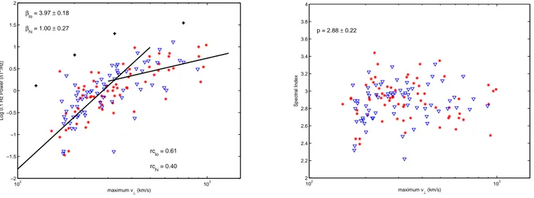
2526 M. Volwerk et al.: Multi-scale turbulence analysis 102 103 −2 −1.5 −1 −0.5 0 0.5 1 1.5 2 βlo = 3.97 ± 0.18 rc lo = 0.61 Log 0.1 Hz Power (nT 2/Hz) maximum v⊥ (km/s) βhi = 1.00 ± 0.27 rc hi = 0.40 102 103 2 2.2 2.4 2.6 2.8 3 3.2 3.4 3.6 3.8 4 p = 2.88 ± 0.22 Spectral Index maximum v⊥ (km/s)
Fig. 1. The top panel shows the low frequency turbulence for 0.08≤f ≤1 Hz for 68 intervals of 12 min near the neutral sheet. The left
panel shows the total power in the turbulence as a function of the maximum perpendicular flow velocity during the 12-min interval. The stars and triangles represent C1 and C3, respectively. The pluses show the velocity dependence of the spectral power determined by Bauer et al. (1995a) for the frequency interval 0.03≤f ≤0.13 Hz. The velocity dependence of the spectral power is fitted for velocity intervals 150≤v⊥,max≤400 km/s and 350≤v⊥,max≤1100 km/s. The bottom panel shows the spectral index as a function of maximum perpendicular flow velocity.
sampling rate of 67 Hz, we will construct a spectral diagram for a broad frequency range, taking into account various de-pendencies on, i.e. the flow velocity of the plasma in the tail.
2 Data analysis techniques
We will first review the data analysis techniques that have been used in the papers that form the basis of this paper. 2.1 High-velocity low-frequency spectral analysis
An analysis of the low-frequency turbulence in the Earth’s current sheet has been performed by Volwerk et al. (2003). They used 12-min intervals of data near the neutral sheet, covering the local time region between 21:00 and 03:00 LT, for both 2001 and 2002. The data were transformed to a mean field-aligned coordinate system. The spectral analysis was performed on 2 Hz sampled data, giving a Nyquist fre-quency of fNy=1 Hz and the spectra were averaged over 7
harmonics with a frequency resolution of 1f =1.4 mHz. It was found that the power in the compressional component was much stronger than the left- and right-hand polarised wave power (see also Bauer et al., 1995a; 1995b; Volwerk et al., 2004). A lower limit was set to the maximum perpen-dicular flow velocity, v⊥,max>150 km/s. Only then does the
frequency interval in which we are interested, 0.08≤f ≤1 Hz, show power above the magnetometer noise level.
A summary plot of all data is shown in Fig. 1. For the turbulent power in the frequency range 0.08≤f ≤1.0 Hz they found that it was highly dependent on the maximum perpen-dicular flow velocity, v⊥,maxmeasured during the interval.
The spectral index of the turbulence is shown to be
p=2.88±0.22 with no dependence on the flow velocity. This value is much larger than Kolmogorov (p=5/3) and close to what one would expect for quasi-2-D turbulence. For pure 2-D turbulence one would expect that p=3 (Frisch, 1995). The occurrence of quasi-2-D turbulence is dependent on a region that is limited in one direction on scales longer than the extension of the region in the third dimension. This is natural for the Earth’s current sheet, which is limited in the
z-direction.
Interestingly it is found that the power in the turbulence can be described as:
P ≡ P (f, v) ∝ f−pvβ, (1)
so not only is there the usual frequency dependence of the spectral power, f−p, but also a velocity dependence
vβ. In the paper by Volwerk et al. (2003) the data were split up in three local time regions: pre-midnight (12:00–23:00 LT); midnight (23:00–01:00 LT) and post-midnight (01:00–03:00 LT). It was shown that two dif-ferent regions could be identified for the velocity depen-dence. For v⊥,max≤400 km/s the turbulent power increases
strongly with slopes βpre=4.51±0.24, βmid=3.82±0.65
and βpost=3.45±0.16 (in the total data set we find
βlo=3.76±0.21, see Fig. 1).
We transform the frequency spectra to wave num-ber space under the assumption that the slope of the spectrum does not change (Borovsky et al., 1997), i.e.
P (f )∝f−p→P (k)∝k−p. This results in a wave spectrum:
where D is the dimensionality of the problem, in this case
D=1 (see Volwerk et al., 2003 for a discussion of this value). This dependence on the flow velocity can be explained when the wave power is generated by a streaming instability, most likely the Kelvin-Helmholtz instability (KHI) on the bound-ary between the flow channel and the ambient magneto-tail. Transformed to wave number space one finds that the power grows linearly with the maximum velocity (βlo≈3.76,
p≈2.88), what one would expect for the KHI:
˙
P =2γ P with γ ∝ v. (3)
At higher velocities, v⊥,max>400 km/s, the spectral power
becomes saturated, demonstrated by a much smaller slope for the velocity dependence. For this region it was found that
βpre=1.95±0.20, βmid=1.20±0.45 and βpost=1.44±0.50 (in
the total data set we find βhi=1.06±0.48, see Fig. 1). One
finds that the spectral power becomes independent from the flow velocity or even inversely dependent on it (βhi≈1.06,
p≈2.88), showing clearly the saturation of the generating instability. Indeed, Melrose (1986) states that “if the KHI develops too fast, the resuling turbulent mixing can reduce the shear below this threshold, thereby suppressing the insta-bility”.
For even lower frequencies f ≤0.06 Hz, containing the Pi2 band (8–25 mHz), the 12-min intervals are too short to obtain an accurate spectral index. We will return to this frequency band later in the case studies in Sect. 3.
2.2 High-frequency wavelet analysis
In order to investigate higher-frequency turbulence than in the previous section, we cannot suffice with 2-Hz sampled data and just regular spectral analysis. The signals at higher frequencies are embedded in a high noise region. Therefore, for selected events, V¨or¨os et al. (2003; submitted, 20041) studied the normal and burst mode (22 Hz and 67 Hz, respec-tively) magnetic field data with a discrete wavelet technique. Again, a relationship is sought between the spectral power and the frequency:
P (f ) ∝ cff−αS, (4)
where now cf and αSare determined by a wavelet estimator.
This estimator involves a semi-parametric wavelet technique based on a fast pyramidal algorithm, which allows unbiased estimations of the scaling parameters cf and α (Abry et al., 2000). A discrete wavelet transform of the time series is per-formed over a dyadic grid of scale (j ) and time (t) and for each octave the variance µj of the discrete wavelet coeffi-cients is calculated: µj = 1 nj nj X t =1 d2(j, t ) ∝2j αcf, (5)
where nj are the number of coefficients at octave (scale) j and d(j, t ) is the discrete wavelet coefficient. The parame-ters cf and α are then found by linear regression of the log-arithm of the variance µ with respect to the observed scale j
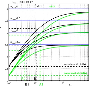
100 101 102 0 0.5 1 1.5 2 2.5 3 α c fsn B X −− 2001−09−07 s/c 1 s/c 3 αmod=1.5 αmod=2 αmod=2.5 αmod=3 noise level s/c 1 (Bx) noise level s/c 3 (Bx) A B B1 A1
Fig. 2. The scaling parameter correction curves for two spacecraft
(C1 and C3) for scale j =4. For known signal-to-noise ratios, cfsn, it is shown from synthetic data that for small values the true scaling
αis recovered incorrectly and needs to be corrected. The graph also shows the difference in noise level for C1 and C3. A, B, A1 and B1 represent the examples studied in the case studies, respectively, for 27 August 2001 and 13 September 2002.
(intercept and slope, respectively); for a full description, see V¨or¨os et al. (2004). We choose to describe the “spectral in-dex” by αS, to clarify the different analysis technique used.
As at higher frequencies the signal-to-noise ratio becomes very small; a check of the feasibility of this procedure is needed. Therefore, V¨or¨os et al. (submitted, 20041) have used quiet magnetotail intervals and embedded artificial nals, with known scaling parameters and reminiscent of sig-nals expected to be found in the magnetotail, and performed the wavelet analysis to find these scaling parameters. It was shown that depending on the signal-to-noise ratio, cfsnand on
the scale j , recovery of the scaling parameters was possible. For different frequency ranges (or scales j ) the time win-dow used was optimized to recover the synthetic signals. By varying the signal-to-noise level, the known scaling pareme-ters were recovered with varying accuracy, and were usually underestimated. The correction curves showed the correct value of αSfor a measured αS,m. Covering a large parameter
space of cfsnand j , V¨or¨os et al. (submitted, 20041) created
these correction curves which can be applied to the deter-mination of the scaling parameters from active magnetotail data. The correction curves were computed by embedding artificial signals to quiet time measurements on 7 September 2001. Examples of these curves for C1 and C3 can be seen in Fig. 2, and these curves will be used in this paper.
The main problems in this process are: determining the signal-to-noise ratio, cfsn (the noise level for each
2528 M. Volwerk et al.: Multi-scale turbulence analysis −5 0 5 10 15 20 25 30 0 0.5 1 1.5 2 2.5 3 0 3 6 9 12 0130 0200 0230 0300 0330 0400 0430 0500 −600 −400 −200 0 200 400 600 BX (j3,j4) (j1,j2) α c fsn V⊥x [nT] [km/s] 2001−08−27 s/c 1 s/c 3 UT A B
Fig. 3. Top panel: The Bxfor 27 August 2001, for C1 (black) and C3 (green). Next panel: The wavelet scaling parameter α for scales
(j1, j2)and (j3, j4). Next panel: The signal-to-noise estimator cfsn defined as the relative power of intercepts cfsn=cactivity/<cnoise>. Bottom panel: x-component of the perpendicular flow velocity. The correction of the scaling parameter αS for A and B are shown in Fig. 2.
wavelet transform is performed. The latter problem can be solved by using a synthetic data set and for each scale the op-timal width of the window can be found by trial. The differ-ent noise levels for each spacecraft can be determined. This makes sure that each spacecraft has its own set of correction curves, as shown in Fig. 2. The first problem is not so trivial, but using the data one can construct a quantity determined by the “relative power of intercepts” from the wavelet analysis. In the wavelet scalogram the intercept at scale j =0 is deter-mined for the noise (from the quiet time data) and for active data, i.e. the cfs describing the spectral power P (f ). From
analysis of synthetic data one finds that this relative power of intercepts, cfsn=cactivity/hcnoisei, is an adequate quantity
to describe the signal-to-noise ratio. We note that hcnoiseiis
independent of the location of the Cluster spacecraft; for fur-ther details, see V¨or¨os et al. (submitted, 20041).
For selected intervals containing bursty bulk flows (BBFs; see, e.g. Baumjohann et al., 1990; Angelopoulos et al., 1994) the (corrected) scaling parameters have been determined. It is found that in the absence of flow in the magnetotail cfsn≈1,
and only during fast flows does one find that cfsn>1 and is
scaling information available. From the correction curves in Fig. 2 it is clear that for cfsn 100 the scaling parameter α
for small scales (j1, j2)=(0.08, 0.33) s needs to be corrected,
Table 1. Statistical evaluation of large-scale αLS for 27 August 2001, for two different conditions. Cond. 1: Based on small scales: BBF when αSS>0.9 and cfsn>2; non-BBF when αSS<0.4 and
cfsn<1.1; Cond. 2: Based on perpendicular velocity: BBF when
v⊥,xy>300 km/s; non-BBF when v⊥,xy<100 km/s. Bx By Bz C1 C1 C1 Cond. αLSBBF 2.55±0.04 2.56±0.06 2.53±0.08 1 αLSnon-BBF 1.7±0.3 2.1±0.3 2.1±0.2 Cond. αLSBBF 2.6±0.1 2.6±0.1 2.6±0.1 2 αLSnon-BBF 1.9±0.3 2.1±0.3 2.1±0.3 C3 C3 C3 Cond. αLSBBF 2.59±0.04 2.59±0.04 2.52±0.06 1 αLSnon-BBF 1.6±0.4 1.8±0.4 1.9±0.2 Cond. αLSBBF 2.6±0.1 2.6±0.1 2.5±0.1 2 αLSnon-BBF 1.5±0.4 1.7±0.4 2.0±0.3
whereas at larger scales (j3, j4)=(0.7, 11) s the scaling
pa-rameters can be trusted. The cfsnseems to correlate best with
the perpendicular plasma flow, v⊥.
Figure 3 shows the wavelet analysis results for Bxfor 27
August 2001. During the interval 01:10–05:00 UT on 27 August 2001, the Cluster spacecraft were near the zGSM=0
plane, in the post-midnight magnetotail (xGSM∼−19 RE). The correlation between v⊥and cfsnis clear, whenever there
are BBFs the signal-to-noise ratio increases. This is similar to what was observed in the low-frequency turbulence, where the perpendicular flow velocity had to exceed 150 km/s for the whole frequency interval to show power above the noise level. The results from the wavelet analysis can be found in Table 1. Two different kinds of conditions are put onto the data:
1. Based on small scales: BBF when αSS>0.9 and cfsn>2;
non-BBF when αSS<0.4 and cfsn<1.1;
2. Based on perpendicular velocity: BBF when
v⊥,xy>300 km/s; non-BBF when v⊥,xy<100 km/s.
For both conditions on the data we find that for BBF type of data the scaling αLS≈2.6, where the large scale indicates
time scales of 0.7–11 s or frequency scale of 1.4–0.09 Hz, overlapping with the spectral analysis region in the previous section. Indeed, we find that during fast flows the scaling index is similar between the two methods (i.e. spectral anal-ysis and wavelet analanal-ysis), 2.88±0.22 and 2.6±0.1. In the case of non-BBF periods we find that 1.5≤αLS≤2.1, which
is very close to a Kolmogorov spectrum (αkol=5/3).
For the smaller scales, i.e. (j1, j2)=(0.08, 0.33) s, or
for the frequency range 12.5–3 Hz it was found that the
cfsn 100 (see Fig. 3); thus the values for αSSmust be
cor-rected using the curves in Fig. 2. This shows that for the identified regions of BBFs the wave power can be described
−20 −10 0 10 20 30 Bx −20 −10 0 10 20 30 By −20 −10 0 10 20 30 Bz 1 1.5 2 2.5 3 3.5 4 4.5 5 5.5 6 0 10 20 30 Bm UT 10−3 10−2 10−1 100 10−2 10−1 100 101 102 103 104 Frequency (Hz) pC1 = 1.86 Power (nT 2/Hz)
Fig. 4. Top panel: magnetic field data for 27 August 2001, in GSM
coordinates for all spacecraft, colour coded in the following way: C1 black, C2 red, C3 green and C4 blue. Bottom panel: The power spectra of the compressional components of the magnetic field for C1. The spectral power is fitted with respect to frequency over the interval 0.005≤f ≤0.04 Hz to obtain a low-frequency spectral index and shown as the solid straight line. The arrows depict the different frequency ranges: the low frequency fit range (long arrow left), the Pi2 frequency band (short arrow left) and the high-frequency range (long arrow right).
by αSS≈2.6, similar to what was found for the larger scale
(j3, j4). In the case of no BBF activity the wavelet analysis
shows that cfsn≈1, which means that only noise is measured
and thus, we can conclude that there is no significant energy flow to small scales.
3 Case studies
We will study in more detail two extended periods with the Cluster spacecraft near the neutral sheet, during sub-storm times, and with the availability of burst mode (67 Hz) magnetic field data. The days are: 27 August 2001, 01:00–06:00 UT (burst mode data for 01:30–03:00 UT) and 13 September 2002, 17:00–23:00 UT (burst mode data for
−20 −10 0 10 20 30 Bx −20 −10 0 10 20 30 By −20 −10 0 10 20 30 Bz 17 18 19 20 21 22 23 0 10 20 30 Bm UT 10−3 10−2 10−1 100 10−2 10−1 100 101 102 103 104 Frequency (Hz) pC1 = 2.64 Power (nT 2/Hz)
Fig. 5. Magnetic field data and power spectrum for 13 September
2002, for details, see caption Fig. 4.
18:00–20:00 UT). Some of the results for the first interval have already been discussed in the previous section.
The magnetic field data for 27 August are given in Fig. 4. With a long time interval there is enough spectral resolution to fit the low-frequency region of the spectrum. We choose a frequency interval 0.005≤f ≤0.06 Hz. We find that we can describe the spectrum with a spectral index p=1.8. This is flatter than the higher frequency interval 0.08<f <1.0 Hz, which is described by a spectral index of p=2.8.
For the spectral power at higher frequencies we need the wavelet analysis approach. In the previous section we found that the description of the spectral power was dependent on the presence of BBF activity. For BBF intervals we find that for 0.09≤f ≤1.4 Hz the wavelet scaling is described by
αLS≈2.6 and for 3.0≤f ≤12 Hz the scaling is described by
αSS≈2.6 as well, indicating that there is no break in the
power spectrum between these two frequency ranges. On the other hand, for the non-BBF intervals it was found that 1.5≤αLS≤2.1 and for higher frequencies the signal-to-noise
ratio was too small to obtain a result.
The magnetic field data for 13 September 2002 are given in Fig. 5. Using spectral analysis we find that for the
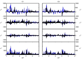
2530 M. Volwerk et al.: Multi-scale turbulence analysis −500 0 500 1000 vx C1 −500 0 500 vy −500 0 500 vz 1 2 3 4 5 6 0 500 1000 1500 vt UT −500 0 500 1000 vx C3 −500 0 500 vy −500 0 500 vz 1 2 3 4 5 60 500 1000 1500 vt UT
Fig. 6. The plasma flow velocity for 27 August 2001, with the
per-pendicular component shown as the filled curve underneath, for C1 and C3. −500 0 500 1000 vx C1 −500 0 500 vy −500 0 500 vz 17 18 19 20 21 22 23 0 500 1000 1500 vt UT −1000 −500 0 500 vx C3 −500 0 500 vy −500 0 500 vz 17 18 19 20 21 22 230 500 1000 1500 vt UT
Fig. 7. The plasma flow velocity for 13 September 2002, with the
perpendicular component shown as the filled curve underneath, for C1 and C3.
low-frequency region of the spectrum the wave power can be described by p≈2.6, and the higher frequency range has a similar slope, indicating that there is no break in the spec-trum. This is a notable difference from the slope for 27 Au-gust 2001, where such a break was found and which is also described in Hoshino et al. (1994) and Volwerk et al. (2004). The break in the power spectrum near f ≈0.08 Hz was ex-plained by the finite thickness of the fast flow channel. Vol-werk et al. (2003) assumed a thickness of 4000 km for the flow channel and found that magneto-acoustic waves would have an “eigenmode” at a frequency f ≈0.06 Hz.
A clear difference between 27 August 2001 and 13 September 2002 can be seen in Figs. 6 and 7. The latter day has a much shorter interval of strong flow activity. In-deed, when we perform spectral analysis on the data from 13 September 2002, for the interval 19:00–23:00 UT, i.e. take out the strong flow bursts, the spectral index remains approx-imately the same. Only the total spectral power decreases
Table 2. Statistical evaluation of large-scale αLS for 13 Septem-ber, 2002, for two different conditions. Cond. 1: Based on small scales: BBF when αSS>0.9 and cfsn>2; non-BBF when αSS<0.4 and cfsn<1.1; Cond. 2: Based on perpendicular velocity: BBF when v⊥,xy>300 km/s; non-BBF when v⊥,xy<100 km/s.
Bx By Bz C1 C1 C1 Cond. αLSBBF 2.3±0.2 2.2±0.2 2.4±0.3 1 αLSnon-BBF 1.0±0.3 1.2±0.3 2.0±0.1 Cond. αLSBBF 2.42±0.15 2.5±0.2 2.4±0.2 2 αLSnon-BBF 1.3±0.5 1.7±0.5 2.2±0.2 C3 C3 C3 Cond. αLSBBF 2.5±0.2 2.3±0.2 2.3±0.3 1 αLSnon-BBF 0.9±0.4 1.0±0.5 1.3±0.5 Cond. αLSBBF 2.5±0.1 2.4±0.2 2.6±0.1 2 αLSnon-BBF 1.4±0.6 1.5±0.6 1.6±0.6
by a factor ∼2. Apparently, the presence of a flow channel is necessary for the creation of a break in the power spec-trum. Without limited z-dimensions the magneto-acoustic waves can propagate over the whole current sheet, creating a coupling between small and large scales.
The results of the wavelet analysis of 13 September 2002 are shown in Fig. 8 and the statistical evaluation of the large-scale αLS for this event are listed in Table 2. The observed
interval in burst mode is shorter than for the previous case (∼2 h vs. ∼4 h). It is clear from Fig. 8 that there are only a few intervals with flow activity. This indicates that the statis-tics are not as good as in the previous case.
Based on the same condition criteria as above, the data are split up into BBF and non-BBF events. Again, it is shown that BBF events after correction show scaling parameters
αLS≈2.4. For non-BBF events the determination of αLS
be-comes difficult, as cfsnbecomes very small and the correction
curves in Fig. 2 are very close together.
4 Multi-scalar turbulent spectrum
Combining all the results from above we can come to a full description of the turbulent wave spectrum. Naturally we have to take into account the different conditions of the cur-rent sheet to obtain such a description. From our results above the spectral index can be very different depending on the flow activity. We list the spectral index p and scaling parameter αSin Table 3.
Using the values in Table 3 we can obtain a multiscale spectrum of the turbulence in the current sheet. Indeed, we can now put values to the posited spectrum by Zelenyi et al. (1998) and expand on the power spectrum presented by Borovsky and Funsten (2003) (but note that Borovsky and Funsten investigate totally different magnetospheric condi-tions, magnetotail compression by northward IMF magnetic
Table 3. The spectral indices p and scaling parameters αSas deter-mined from the spectral and wavelet analysis. Average values for flow and no-flow intervals are given.
Freq. Range flow no-flow flow no-flow
Hz p p αS αS
0.005≤f ≤0.04 ∼1.8 ∼2.8 NA NA 0.08≤f ≤1.0 ∼2.8 NA ∼2.6 NA 3.0≤f ≤12.5 NA NA ∼2.6 ∼1.8
clouds, whereas we investigate substorm-related phenom-ena). We find that there is one possible spectral break at
f1≈0.08 Hz, and no real evidence for a second spectral break
at higher frequencies. The smaller scaling parameter αLSfor
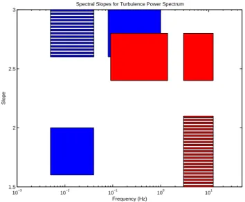
the high frequency range must be regarded critically, as the signal-to-noise ratios for non-BBF events are very small and thus, some of the information in the data may be lost in the noise. In Fig. 9 we show the results as obtained in this paper. The solid boxes show the slopes for BBF conditions and the striped boxes for non-BBF conditions. The shaded regions show the possible variation in slopes as given by the error bars.
5 Discussion
We have investigated the spectral power scaling with respect to frequency for the magnetic wave activity observed in the Earth’s tail current sheet. It was proposed that in the power spectra there would be two breaks at frequencies usually la-belled f1 and f2or f∗and f∗∗. It was shown by Hoshino et al. (1994) that f1≈0.04 Hz and similarly by Volwerk et al.
(2004) that f1≈0.08 Hz and Bauer et al. (1995a) noticed a
break in the spectrum f1≈0.03 Hz. This seems to be a well
established frequency range for f1. However, Zelenyi et al.
(1998) studied the z-component of the magnetic field and found that it showed a “two-kink behaviour” with turn-over frequencies f∗≈0.01 Hz and f∗∗≈0.25 Hz. This is not in agreement with the results presented in this paper. It is not feasible to put f1≡f∗. Also, our results show no indication of a break at f∗∗≈0.25 Hz.
An interesting detail in our results is that in the frequency range 0.08≤f ≤1 Hz, which was investigated both by Fourier spectral analysis and wavelet analysis, the spectral index was 2.6 and 2.8, respectively. In the intermediate frequency range there is strong overlap between the powers determined from spectra and wavelet analyses under flow conditions, suggest-ing that the spectral index is more of the order of 2.6±0.1. Physically this implies that the turbulence is not strictly two-dimensional in the presence of strong flows, but rather it is intermittent such that the dimensionality is fractal 2<D<3 with scales substantially smaller than the width of the re-gion (in this case the flow channel) in z-direction contribut-ing. The presence of smaller scale structures contributing to the turbulence is also suggested by the index in the
high-−20 −10 0 10 20 0 0.5 1 1.5 2 2.5 3 0 3 6 9 12 15 1800 1830 1900 1930 2000 −800 −400 0 400 800 2002−09−13 BX [nT] α cfsn V⊥ X [km/s] UT A1 B1 (j1,j2) (j3,j4)
Fig. 8. Wavelet analysis of the data from 13 September 2002 in
similar form as Fig. 3. The correction of the scaling parameter αS for A1 and B1 are shown in Fig. 2.
10−3 10−2 10−1 100 101 1.5 2 2.5 3 Frequency (Hz) Slope
Spectral Slopes for Turbulence Power Spectrum
Fig. 9. A schematic for the slope of the power spectrum as deduced
in this paper for different frequency ranges, determination methods and flow activity. Blue: Spectral analysis; Red: Wavelet analysis. The solid boxes are for BBF intervals and the striped boxes are for non-BBF periods. For the numerical values of the slopes, see Ta-ble 3.
frequency range found from the wavelet analysis, which is identical to that in the intermediate frequency range, suggest-ing no spectral break at those higher frequencies.
It is interesting to also comment on the flat Kolmogorov-like spectra obtained from the spectral analysis in the very low-frequency range. This quasi-three-dimensional
2532 M. Volwerk et al.: Multi-scale turbulence analysis character of the turbulence here suggests that scales
con-siderably larger than the width of the region under consid-eration are involved at those frequencies. The local prop-erties and in particular the boundedness of the region in the z-direction does not substantially affect the turbulence here. The strong spectral break at f ≈0.08 Hz, where the spectrum changes from the flat Kolmogorov-like spectrum to the steep quasi-two-dimensional intermittent fractal turbu-lent spectrum, shows the transition from scales which ignore those that recognize the effect of the boundedness of the re-gion in z.
The spectral behaviour under no-flow conditions shows the transition from quasi-two-dimensional turbulence at low frequencies to Kolmogorov-like turbulence at high frequen-cies. Since under these conditions the spectrum cannot be resolved by wavelet analysis, as mentioned earlier, the inter-mediate region index is lacking. However, if real, the break from steep, low-frequency 2-D turbulence to flat, high fre-quency 3-D turbulence indicates that the larger scales at low frequency are sensitive to the boundedness of the region. The smaller scales at high frequency are clearly independent of the presence of the boundaries of the region such that their behaviour is three-dimensional. The obvious conclusion that can be drawn from this mutual behaviour under no-flow and under flow conditions is that the turbulent region detected un-der no-flow conditions is wiun-der in the z direction than unun-der flow conditions. Under high flow conditions the region of the plasma sheet that behaves turbulently must be thin compared to the conditions when no flows are detected. Nakamura et al. (2002) discusses the thinning of the current sheet during fast flows.
We note that the indices found in this paper are higher than previously estimated, where it was found that the spectral in-dex is 2–2.5 (Bauer et al., 1995a), 2.2 (Borovsky et al., 1997) and 1.78–2.43 (Zelenyi et al., 1998, with no reference for the very low 1.78 given). This need not be surprising, as our data sets were highly selected with strong criteria on magnetic field strength and flow velocity. Volwerk et al. (2003) showed that if the flow velocity was too low (v⊥,max<150 km/s) the
power in the higher-frequency part of the interval 0.08–1 Hz disappeared into the noise level of the magnetometer, and thus, artificially reduced the spectral index.
Unfortunately, we cannot give a value for f2at which the
next break in the spectrum would occur. The possible break at f ≈3 Hz that can be seen in Fig. 9 cannot be interpreted as such. The change in scaling index αSS depends on the
presence of BBFs. If there is no flow, then the signal-to-noise ratio is very small, and we lose information about the scaling index. The noise tends to flatten the slope of the spectrum, which is an artifact, and does not represent the true scaling index of the high-frequency turbulence. Therefore, we have to conclude that f2 probably resides at a higher frequency
than shown in the figure, in a region where we are unable to significantly investigate the data.
The periods of non-BBF show different characteristics. In the low frequency we see that the slope is steep (p≈2.8), in-dicating that there is transport of turbulent power to larger
scales, what one would expect for 2-D turbulence. In the high-frequency range, however, we see a flatter slope (p≈1.8), indicating that there is no transport of turbulent power to these scales. The latter introduces an artificial break in the power spectrum, which is related to the signal disap-pearing into the noise level and not with a physical process as in the lower frequency range.
Acknowledgements. We would like to acknowledge the Cluster
Sci-ence Data System (CSDS). The authors ould like to thank H.-U. Eichelberger and Y. Bogdanova for preparing the Cluster FGM and CIS data. The work by MV and KHG was financially supported by the German Bundesministerium f¨ur Bildung und Forschung and the Zentrum f¨ur Luft- und Raumfahrt under contracts 50 OC 0104 and 50 OC 0103, respectively.
Topical Editor T. Pulkkinen thanks a referee for his help in eval-uating this paper.
References
Abry, P., Flandrin, R., Taqqu, M. S., and Veitch, D.: Self-similar network traffic and performance, Wiley Interscience, New York, 2000.
Angelopoulos, V., Kennel, C. F., Coroniti, F. V., Pellat, R., Kivel-son, M. G., Walker, R. J., Russell, C. T., Baumjohann, W., Feld-man, W. C., and Gosling, J. T.: Statistical characteristics of bursty bulk flow events, J. Geophys. Res., 99, 21 257–21 280, 1994.
Balogh, A., Carr, C. M., Acu˜na, M. H., Dunlop, M. W., Beek, T. J., Brown, P., Fornacon, K.-H., Georgescu, E., Glassmeier, K.-H., Harris, J., Musmann, G., Oddy, T., and Schwingenschuh, K.: The Cluster magnetic field investigation: overview of in-flight performance and initial results, Ann. Geophys., 19, 1207–1217, 2001.
Bauer, T. M., Baumjohann, W., Treumann, R. A., Sckopke, N., and L¨uhr, H.: Low-frequency waves in the near-Earth plasma sheet, J. Geophys. Res., 100, 9605–9617, 1995a.
Bauer, T. M., Baumjohann, W., and Treumann, R. A.: Neutral sheet oscillations at substorm onset, J. Geophys. Res., 100, 23 737– 23 743, 1995b.
Baumjohann, W., Paschmann, G., and L¨uhr, H.: Characteristics of high-speed flows in the plasma sheet, J. Geophys. Res., 95, 3801–3809, 1990.
Borovsky, J. E. and Funsten, H. O.: MHD turbulence in the Earth’s plasma sheet: Dynamics, dissipation, and driving, J. Geophys. Res., 108(A7), 1284, doi:1.1029/2002JA009625, 2003. Borovsky, J. E., Elphic, R. C., Funsten, H. O., and Thomsen, M. F.:
The Earth’s plasma sheet as a laboratory for flow turbulence in high-β MHD, J. Plasma Phys., 57, 1–34, 1997.
Frisch, U.: Turbulence, Cambridge University Press, Cambridge, UK, 1995.
Hoshino, M., Nishida, A., Yamamoto, T., and Kokubun, S.: Turbu-lent magnetic field in the distant magnetotail: Bottom-up process of plasmoid formation?, Geophys. Res. Lett., 21, 2935–2938, 1994.
Melrose, D. B.: Instabilities in space and laboratory plasmas, Cam-bridge University Press, 1986.
Nakamura, R., Baumjohann, W., Runov, A., Volwerk, M., Zhang, T. L., Klecker, B., Bogdanova, Y., Roux, A., Balogh, A., R`eme, H., Sauvaud, J. A., and Frey, H. U.: Fast flows
dur-ing current sheet thinndur-ing, Geophys. Res. Lett., 29, (29), 2140, doi:10.1029/2002GL016200, 2002.
R`eme, H., Aoustin, C., Bosqued, J., et al.: First multi-spacecraft ion measurements in and near the Earth’s magnetosphere with the identical Cluster ion spectrometry (CIS) experiment, Ann. Geophys., 19, 1303–1354, 2001.
Sigsbee, K., Cattell, C. A., Moser, F. S., Tsuruda, K., and Kokubun, S.: Geotail observations of low-frequency waves from 0.001 to 16 Hz during the November 24, 1996, geospace environment modelling substorm challenge event, J. Geophys. Res., 106, 435– 445, 2001.
Volwerk, M., Nakamura, R., Baumjohann, W., et al.: A statistical study of compressional waves in the tail current sheet, J. Geo-phys. Res., 108, (A12), 1429, doi:10.1029/2003JA101155, 2003. Volwerk, M., Baumjohann, W., Glassmeier, K.-H., Nakamura, R., Zhang, T. L., Runov, A., V¨or¨os, Z., Klecker, B., Treumann, R. A., Bogdanova, Y., Eichelberger, H.-U., Balogh, A., and R`eme, H.: Compressional waves in the Earth’s neutral sheet, Ann. Geo-phys., 22, 303–315, 2004.
V¨or¨os, Z., Baumjohann, W., Nakamura, R., Runov, A., Zhang, T. L., Volwerk, M., Eichelberger, H. U., Balogh, A., Horbury, T. S., Glassmeier, K.-H., Klecker, B., and R`eme, H.: Multi-scale magnetic field intermittence in the plasma sheet, Ann. Geophys., 21, 1955–1964, 2003.
V¨or¨os, Z., Baumjohann, W., Nakamura, R., Runov, A., Volwerk, M., Zhang, T. L., and Balogh, A.: Wavelet analysis of magnetic turbulence in the Earth’s plasma sheet, Phys. Plasmas, 11, 1333– 1338, 2004.
Zelenyi, L., Milanov, A. V., and Zimbardo, G.: Multiscale magnetic structure of the distant tail: Self-consistent fractal approach, New perspectives on the earth’s magnetotail, Geophys. Monogr. Ser., 105, edited by Nishida, A., Baker, D. N., and Cowley, S. W. H., AGU, Washington, DC, USA, 321–339, 1998.