HAL Id: hal-01518560
https://hal.archives-ouvertes.fr/hal-01518560
Submitted on 4 May 2017
HAL is a multi-disciplinary open access
archive for the deposit and dissemination of
sci-entific research documents, whether they are
pub-lished or not. The documents may come from
teaching and research institutions in France or
abroad, or from public or private research centers.
L’archive ouverte pluridisciplinaire HAL, est
destinée au dépôt et à la diffusion de documents
scientifiques de niveau recherche, publiés ou non,
émanant des établissements d’enseignement et de
recherche français ou étrangers, des laboratoires
publics ou privés.
Scalable photon splatting for global illumination
Fabien Lavignotte, Mathias Paulin
To cite this version:
Fabien Lavignotte, Mathias Paulin. Scalable photon splatting for global illumination. 1st
Interna-tional conference on Computer graphics and interactive techniques in Australasia and South East
Asia (GRAPHITE’03), Feb 2003, Melbourne, Australia. pp.203 - 213, �10.1145/604471.604511�.
�hal-01518560�
Scalable Photon Splatting for Global Illumination
Fabien Lavignotte Mathias Paulin IRIT University Paul Sabatier
Toulouse France
Abstract
In this paper, we present a new image based method for computing efficiently global illumination using graphics hardware. We pro-pose a two pass method to compute global lighting at each pixel. In the first pass, photons are traced from the light sources and their hit points are stored. Then, in the second pass, each photons hit point is splatted on the image to reconstruct the irradiance. The main ad-vantages of our method in comparison with previous approaches is scalability. Indeed, it can be used to obtain coarse solution as well as accurate solution and is well suited for complex scenes. First, we present the density estimation framework that is the theory behind our reconstruction pass to understand how to control the accuracy with our method. Then, we show how to use graphics hardware to improve reconstruction time with some restrictions but without losing the ability to compute an accurate simulation.
CR Categories: I.3.7 [Computer Graphics]: Three-Dimensional
Graphics and Realism—Radiosity;
Keywords: global illumination, density estimation, graphics hardware, photon tracing
1
Introduction
The goal of global illumination is to resolve the light transport inte-gral [Kajiya 1986] to generate a photorealistic image from a scene description. Algorithms based on unbiased Monte Carlo methods have been proposed to resolve the light transport integral. They consist in sampling the transport paths from the light sources to the camera lens. Clever sampling of the light transport paths allow to represent various complex lighting effects such as caustics, soft shadows, glossy reflections and indirect diffuse lighting [Veach and Guibas 1995] [Veach and Guibas 1997]. But these methods are time consuming and images are still noisy even after sampling a large number of light transport paths because of the slow convergence of Monte Carlo methods.
Multi-pass methods resolve the lack of efficiency in pure Monte Carlo techniques. Some parts of the light transport integral are com-puted using biased but more efficient method, as radiosity to take into account diffuse indirect lighting [Chen et al. 1991] or particle tracing to render caustics on planar surfaces using texture [Heckbert 1990]. The purpose of multi-pass methods is to present a good bal-ance between slow and accurate algorithm and efficient but biased
method. Nevertheless, the biased method must be consistent. Currently, the most popular multi-pass method is the photon map [Jensen 1996]. First, a photon tracing pass generates a set of pho-tons hit points stored in a balanced kd-tree. In fact, two sets, called photon map, are generated : a global photon map to reconstruct in-direct lighting, and a high density caustic photon map to reconstruct caustics. Then, a Monte Carlo ray tracer is used to compute direct lighting and reflections. Radiance is reconstructed from the pho-ton map using nearest neighbor density estimation, nearest phopho-tons being efficiently located using the kd-tree.
The drawback of photon map is that the set of photons hit points must be stored in main memory during the second pass, so the ac-curacy of the photon map is limited. A method has been proposed to control the storage of the photons [Suykens and Willems 2000], avoiding the store too many photons in region of high density. This is still a drawback for the global photon map since a large number of photons is needed. So, to overcome this problem, the photon map estimate for indirect lighting is used only after a first bounce or gathering step, but the final gathering step must be highly sam-pled to avoid noisy artifacts. To be more efficient, some methods avoid to recompute the final gathering step at each pixel [Ward and Heckbert 1992] [Christensen 1999]. The error of these methods is quite difficult to control.
In this paper, we propose a new technique to reconstruct diffuse and caustic lighting effects using a two pass method quite similar to photon mapping. First, we simulate light transport by a pho-ton tracing pass, and then lighting is reconstructed using an image based method that takes advantages of current graphics hardware. Our method is based on photon splatting method [Sturzlinger and Bastos 1997]. This preliminary approach had problems with ac-curacy of reconstruction and was limited to simple scene. So, our goal is that photon splatting becomes a useful tool in global illu-mination so we try to resolve these problems in this paper. First, we present the theory behind our algorithm : the density estimation framework [Walter 1998]. Then, we show how to implement our method on graphics hardware without losing accuracy even with a large number of photons hit points. Also, we present how to re-construct accurately discontinuities features of the lighting such as caustics using adaptive reconstruction. Last, some implementation details and practical applications of our algorithm are given.
2
Density estimation framework
Density estimation framework is composed of two basic phases : a photon tracing phase and a reconstruction phase based on den-sity estimation. The denden-sity estimation framework is related to many different methods : highly accurate view independent solu-tion [Walter 1998], indirect lighting textures [Myszkowski 1997], caustics only textures [Heckbert 1990] [Granier et al. 2000], and photon map [Jensen 1996].
2.1 Photon tracing
Photon tracing consists in tracing random walks or paths from the light sources. The name of photons is a bit misleading because
actually our ’photons’ does not match any physical meaning. A photon is a vertex of a random walk, it consists of a position x, a direction w and an associated weightφor ’power’.
The photons are generated from the light sources according to a probability density function pe(x,ω,λ) where x is the initial
posi-tion of the photon,ωits initial direction andλ its wavelength. The powerφcarried by a photon for a particular wavelength is then :
φ=Le(x,ω,λ) cosθ
N pe(x,ω,λ)
(1) where Leis the self-emitted radiance,θ is the angle between the
normal of the surface at x and the directionω, and N is the number of photons traced from the light sources. Then the photon is traced in the scene and when a photon hit a surface, its hit point y is stored for the next phase. At y, the photon is either absorbed or reflected according to the BRDF using russian roulette. If reflected the new powerφ0carried by the photon is :
φ0= f(y,ω0,λ) cosθ0
pr(y,ω0,λ) φ
where f is the BRDF,ωis the incoming direction,ω0the new di-rection of the photon chosen with the probability density function
pr(y,ω0,λ) andθ0the angle betweenωandω0.
Probability density function are chosen in order to give the same importance for each photon. That means each photon carry the same power.
pe(x,ω,λ) ∼ Le(x,ω,λ) cosθ
pr(y,ω0,λ) = f (y,ω,λ) cosθ0
In the MGF standard, the self-emitted radiance is defined as con-stant in position and direction for each geometric primitive. With this assumption, peis defined as follow. First, the wavelength is
chosen according to a pdf p(λ), a light is selected using the pdf
ΦL(λ)
ΦT(λ). Then the point x is selected uniformly on the light using
pdf A1
L, and finally the directionωis chosen according to the pdf
cosθ
π . As a result using (1), the powerφfor a particular wavelength
is simplified to: φ= ΦT(λ)Le(λ)ALπ Npp(λ)ΦL(λ) = ΦT(λ) Npp(λ) (2) 2.2 Density Estimation
Once the photon tracing phase is completed, the irradiance is re-constructed using the stored photon hit points. This is equivalent to a density estimation problem as shown first by Heckbert [Heck-bert 1990]. Indeed, the photon hit points are distributed accorded to a probability density function p(x,λ) that is proportional to the irradiance E(x,λ):
p(x,λ) =R E(x,λ)
SE(y,λ)dy
(3) The integration of the irradiance in the environment can be replaced by nφ with n the total number of photons andφ the power car-ried by each photon for a specific wavelength. Because this pdf is unknown, a non parametric density estimation is used: the kernel density estimation [Silverman 1986].
The kernel density estimator constructs an estimate ˆp of an
un-known pdf p from a set of n observed data points X1, ..., Xn:
ˆ p(x) = 1 nhd n
∑
i=1 K(x− Xi h ) (4)where d is the dimension of x, K(x) is a kernel function with unit area, generally symmetric and equal to zero if|x| > 1 and h is the bandwidth or smoothing parameter.
One of the main interesting properties of the kernel density es-timator is the trade-off between variance and bias provided by the bandwidth h. Indeed, the integrated bias is proportional to h2and the integrated variance is proportional to(nh)−1[Silverman 1986]. So, for our problem, (3) and (4) are combined to give the follow-ing estimator for computfollow-ing the irradiance of a surface point x:
E(x,λ) = φ h2 n
∑
i=1 K(x− Xi h ) (5)3
Photon splatting
3.1 PrinciplesOur purpose is to reconstruct the irradiance at each pixels efficiently using the estimator (5).The contribution of any photon hit point X to the estimator at surface point x is:
c(X) = φ
h2K(
x− X
h ) (6)
The kernel function K(x) in the estimator is equal to zero if |x| > 1, that means that the contribution of a photon hit point X to the estimator in x is null if the distance between x and X is above the bandwidth h. So, the irradiance estimator can be evaluated by two different techniques :
• For each pixels, find the photon hit points X which distance from the visible point x is below h and sums their contribution. • For each photon hit points X add its contribution to the
esti-mator of each pixels which distance from X is below h when traced from a light source,
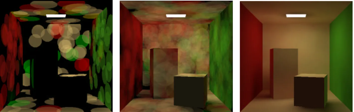
The key observation is that the second technique corresponds to splatting the contribution of each photon hit point onto its surface [Sturzlinger and Bastos 1997]. A splat has the shape of a disc, so the contribution is added to each pixels covered by the projection of the disc into the image and that belong to the same surface. The problem of reconstruction is replaced by a rasterization process. Splatting is performed with graphics hardware using a textured and colored quad. The texture corresponds to a regular sampling of the kernel function and the color is equal to the power of the photons divided by the square of the bandwidth. The final modulated color is then equal to the contribution of the photon. Additive blending is activated to add the contribution of the splat to each pixels. Also, the contribution of a photon must be added only to pixels that be-longs to the same surface it hits. The process is shown in Figure 1 at different level of completion.
3.2 Adjustment to low precision
The principles of photon splatting is quite simple but its implemen-tation on graphics hardware involve difficulties. As explained be-fore, the frame buffer is used to store the estimate at each pixels but frame buffer precision is limited to one byte per channel. It is clearly not sufficient. Photon splatting needs a lot of precision: the contribution of a splat is a triplet of RGB encoded in 32 bit floating point by channel whereas the frame buffer of current graphics hard-ware uses 8 bit fixed point for each channel. The number of non zero contributions from photons hit points are in the order of five hundred so obviously the contribution cannot be scaled to a 8 bit precision. But, using some restriction, frame buffer precision can be sufficient.
Figure 1: Photon Splatting stopped at 0.1% (Left), 1% (Middle) and final (Right).
To adapt to low precision buffer, we choose to use the constant kernel function that is equal to π1. Using constant kernel function is not so a drawback contrary to intuition. It has been shown [Sil-verman 1986] that the kernel function that minimize the mean in-tegrated square error is the Epachenikov kernel Ke. Then, other
kernel functions are compared to Keto measure their efficiency.
A remarkable result is that their efficiencies are close to one. The constant kernel has an efficiency of 0.93. So, for an estimation done with the Epachenikov kernel and with n of random points, n/0.93 random points are needed to obtain the same level of accuracy.
So, the formula (6) is simplified using the constant kernel func-tion:
c(X) = φ
πh2
We will consider for the moment that the powerφand the band-width h is constant for every splat. In result, the contribution of each photon is constant. So, to reconstruct the irradiance at each pixels, we need to compute only the number of contributions, an integer value that can be stored easily in the frame buffer. Once all the photons have been splatted, the irradiance is reconstructed at each pixels(i, j) using the number of contributions Ni jstored in the frame buffer:
E(xi j) = Ni j φ
πh2 (7)
3.3 Choice of the bandwidth
Paragraph 3.2 has shown bandwidth h must be constant to imple-ment photon splatting on a 8 bit frame buffer. In fact, we can choose a constant bandwidth per surface because the splatting is done per surface. The fixed bandwidth h is chosen with an heuristic often used [Shirley et al. 1995] [Sturzlinger and Bastos 1997] :
h= C r
A N
where A is the area of the surface, N the number of photon hit points on the surface and C a user defined constant, usually between 20 and 30.
So, the following algorithm is used:
1. Build an item buffer to obtain the visible surface identifier per pixel.
2. Compute the bandwidth for each surface.
3. Splats each photons using a quad scaled by the bandwidth of its surface.
4. Read the frame buffer and reconstruct the irradiance for each pixels using (7) with bandwidth equals to corresponding visi-ble surface at pixel.
To improve reconstruction of caustics, we also divide the pho-tons set in two parts : caustic and global phopho-tons.The caustic splats use a lower bandwidth, nearly ten times because they are often con-centrated on a small part of the scene. So, step 2 to 4 of the preced-ing algorithm must be repeated for the caustics splats.
3.4 Considerations on photon tracing
As yet, we have considered that the powerφ is constant. As we compute irradiance in RGB color space, there is one constant power for each channel. To accomplish it with photon tracing, one way is to choose for each photon traced from the light sources a channel R,G or B. The channel c is chosen using the following probability density function p(c):
p(c) = ΦT(c)
∑r,g,b
i ΦT(i)
whereΦis the total RGB power of the light sources. Then, using (2), the powerφ(c) for the channel c is :
φ(c) =∑
r,g,b
i ΦT(i)
N
This method is inefficient both for photon tracing and image re-construction because a photon transports power for only one chan-nel. A better solution is that a photon transport a triplet of power for each channel. In this case, the pdf peis not anymore function of
the wavelength or channel. More, the pdf to choose a light source is replaced by : f(ΦL)/ f (ΦT) where f is a function that transforms the triplet of the power into a real value. f can be either the maxi-mum, the average or the luminance of the triplet. A problem for our method is thatφis no longer constant for each splat because some simplifications made in (2) are no longer possible:
φ= f(ΦT)
f(ΦL)
ΦL
N
The resulting formula is dependent of the selected light source, so the power is no longer constant for each splat.
We must use a different approach for our method. First, light sources with the same self-emitted radiance are grouped together. Instead of sending N photons from the light sources, we sent
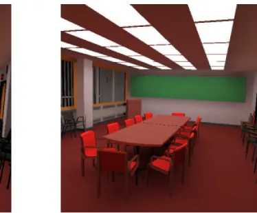
Figure 2: Comparison of two images rendered with photon splatting with boundary bias (Left) and without (Right) Notice the darker regions at boundaries and on small surfaces
f(ΦG)
f(ΦT)N photons from each group of light sources whereΦGis total
power of group G. Using the pdf AL
AG to select a light in the group
G, the powerφGfor each splat is constant for a given group:
φG= ΦG
NG with NG= f(ΦG)
f(ΦT)N
The rendering of the splats is decomposed for each group of light sources. Furthermore, for each light group, the photons transport the powerφG. If the photon hits a surface, it will be rendered as a splat in the reconstruction pass. Because we are only interested in the number of contributions, the color given to the corresponding splat is(1, 1, 1). After hitting a surface, the photon is scattered according to the BRDF at the hit point. The probability of scattering or absorption is done for each channel. The resulting power is the product betweenΦGand a mask(c0, c1, c2) where ciis equals to 1 if scattered, 0 if absorbed. So, if this photon hits a surface again, the color given to the corresponding splat will be equal to the mask.
4
Improving the reconstruction
4.1 Boundary bias
The kernel density estimator assumes that the support of the den-sity function is unbounded. This is not the case in global illumina-tion where the surfaces are bounded. Consequently, energy leaks appear at the boundary of surfaces because irradiance is underesti-mated as shown in Figure 2. The underestimation of the irradiance is an important visual source of error for small surfaces. In order to overcome this problem, the estimator at pixel(i, j) needs to be scaled by Ai j
πh2 i j
where hi jis the bandwidth at(i, j) and Ai jis the in-tersection area between the support of the estimator and the visible surface at(i, j). The support of the estimator is a sphere of radius
hi jcentered on the nearest point visible at(i, j). The computation of the intersection area is a quite complex geometric problem for any kind of input geometry. An implementation with triangle meshes is presented. The algorithm is based on connected triangle mesh:
1. Find a triangle inside the sphere
2. Find the circle deduced from the intersection of the plane of the triangle with the sphere
3. Add the intersection area between the circle and the triangle to the final result
4. Repeat since step 2 on adjacent triangles if their shared edges cross the circle
To avoid cyclic graph on the connected triangle mesh, a mailbox is used on the triangles to know if they have already been visited. It works on complex surfaces as shown in Figure 5.
So, we need to compute the intersection area between a circle and a triangle. First, the triangle is clipped against the circle. In re-sult, a polygon is obtained if the triangle intersects the circle (filled with light gray in Figure 3). The clipping of the triangle introduces segments that are not parallel to the original segments of the trian-gle. These new segments defined half planes. The intersection area between these half planes (filled with dark gray in Figure 3) and the circle is computed and added with the area of the polygon to obtain the intersection area between the circle and the triangle.
Figure 3: Intersection area of a triangle with a circle
4.2 Adaptive image reconstruction
Using a fixed bandwidth per surface blur discontinuities of the ir-radiance as for caustics and shadows for example. Different ap-proaches exist for this problem [Myszkowski 1997] [Walter 1998]. But with our method we cannot use a different bandwidth per pho-ton. But we can generate different images with different bandwidth and choose the best estimator between the set of images. The fol-lowing algorithm is used to allow different bandwidths per pixels:
1. Generate an image estimate using fixed bandwidth per surface 2. For each pixels, an oracle is used to know if the current esti-mate is added to the final image otherwise the pixel is tagged as incorrect
3. If any incorrect pixels remains, compute a new image estimate with the fixed bandwidth reduced by a certain amount and repeat step 2
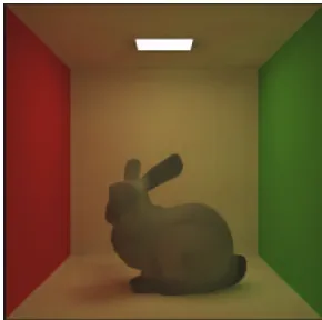
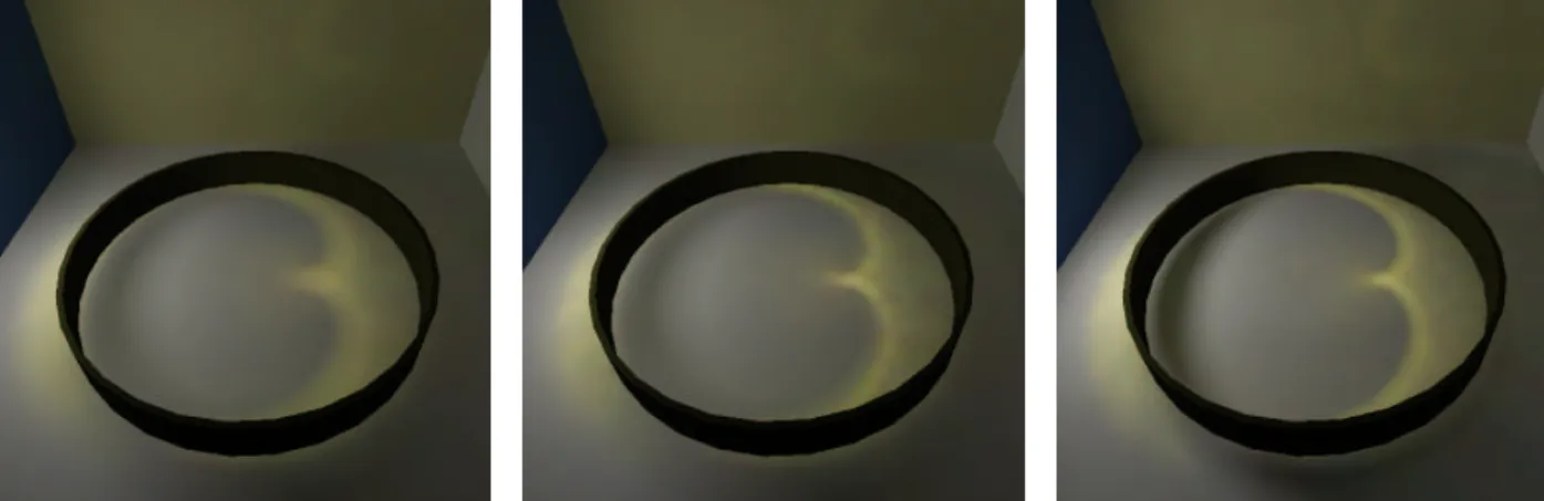
The fixed bandwidth per surface is reduced by one quarter for each subsequent image. The result of the adaptive reconstruction is pre-sented in Figure 4. The adaptive reconstruction has only been done on the caustics splats for efficiency reason. The number of caustics splats is generally sufficiently low compared to the total of splats so the cost of rendering many images is not prohibitive.
4.3 Oracle for bandwidth selection
The oracle should decide for each pixels if its current estimator gives a reasonable level of noise and bias. An often used heuris-tic to estimate the level of noise is based on the number of non zero contributions from the data points. Fortunately, we know this number for each pixel after the splatting phase. So noise can be estimated easily.
To measure bias, our method is based on the fact that the bias of a density function f(x) is proportional to h2f00(x) [Silverman 1986].
From this property, we have deduced that a good way to control the bias would be to limit the bandwidth only in pixels where the second derivative of the estimator is important. As seen in 3.2, the only parameter that vary along the image is the number of non zero contributions Ni j. So, it is sufficient to compute the discrete second derivative of the Ni jusing finite differences. Finite differences are used to compute the partial second derivative in x and y in the image space. Then the maximum value of the partial derivative is taken to measure the bias level. The points pi j of the pixels(i, j) are not regularly spaced in world space. So, we use the formula of second derivative on an irregular grid shown here for the x axis:
∂2N ∂x2 = Ni+1 j− Ni j hi j − fi j− fi−1 j hi−1 j ! hi j+ hi−1 j 2
where hi jis the distance between the point pi j and pi+1 j. This is the central difference formula, but on the boundaries, the backward or forward difference is used.
Our oracle must decide if decreasing the bandwidth will give lower error. First, if variance is already too high, answer is negative. Then, if variance is low, decreasing the bandwidth will decrease bias so answer is positive. Finally, if variance is in the middle range, the value of the second derivative is computed to decide if it is a region of high bias.
Finally, three parameters control the oracle : Nminand Nmax(the
minimum and maximum number of non zero contributions) andε (the threshold for the bias). So, the oracle uses the following con-ditions for a pixel(i, j) : if Ni jis less than Nminor Ni jis less than
Nmaxand the level of bias is underεthen the pixel is correct.
This oracle is quite efficient, the only computation is finite dif-ferences formula which is not complex.
5
Implementation
5.1 Frame buffer overflow
The number of contributions is about five hundreds to two thou-sands, so it overflow the 8 bit value of each channel. To resolve
Figure 5: An example of photon splatting with a complex surface and boundary bias correction
this problem, we need to add periodically the content of the frame buffer to a higher precision buffer after a number of rendered splat and to reset the frame buffer. In OpenGL, the accumulation buffer allows effectively to add the current value of the frame buffer to a higher precision buffer. Unfortunately, it is not supported on many graphics cards and it is very slow if done in software by the drivers. In fact, reading the frame buffer and storing the result in a higher precision buffer at application level is faster than using the software alternative of accumulation buffer provided by the drivers.
To achieve good performance, the data transfer between the graphics card and the CPU memory must be minimized. It is diffi-cult to guess an a priori upper bound on the maximum number of splats that can be rendered before causing a buffer overflow. So, an heuristic is used to decide when to read the frame buffer. The idea is to compute an upper bound on the maximum number of non zero contributions in the frame buffer for the current scene. Then, we divide this number by the maximum value of the frame buffer to obtain the number of steps in the rendering process.
We approximate the probability that a splat adds its contribution to a pixel as the area of the splat over the total area of the scene. So, the maximum number of contributions ˜N per pixel is approximated
as:
˜
N= nπh 2
DAt (8)
where n is the total number of photons hit points, At is the total
surface area of the scene, h the average bandwidth of the surfaces and D a constant between 0.0 and 1.0. Then, we decompose the photon splatting in ˜N/M steps, where M the maximum value in the frame buffer
The constant D is here to take into account that a splat has not equal chance to fall into each region of the scene. Some regions can be occluded with regard to light sources for example. So, D must be approximatively proportional to the percentage of occluded area in the scene. This approximation works if the photon hit points are well distributed in the unoccluded scene. This assumption is violated for caustics lighting effects where the density of photons hit points is high in a particular region. The caustics splats are rendered with a very low value of D as 0.1 for example which means caustics appears only in 10 percent of the scene.
Figure 4: Three images rendered with Left : fixed bandwidth, Middle : adaptive bandwidth, Right : reference solution
5.2 Hardware implementation
The rendering of the splat must be restricted to the visible part of its surface. An implementation with the OpenGL API is presented here.
When OpenGL rasterize a geometric primitive, it converts it into fragments. A fragment corresponds to a pixel in the frame buffer. A series of operations are performed in the fragment before being stored in the frame buffer. The interesting operations for our pur-pose is the several tests a fragment has to pass before going in the frame buffer. Depth test can be used to limit the rendering of the splat to the pixels with same depth values but the precision is not sufficient to test equality even between a splat and a planar surface. Stencil test compares a reference eight bits value to the stencil pixel value. Using equality comparison, stencil test can effectively re-strict the rendering of the splat to surfaces with the same identifier but we are limited to only 255 different surfaces.
Fortunately, the new generation of graphics hardware provides programmable fragment operations often called pixel shader or fragment shads. Several instructions are provided to the program-mer to output the final color that will be stored in the frame buffer. Instructions operates on different RGBA colors registers
r0, r1, ..., rn with input as the primary color or texels fetched from texture units. Only one conditional instruction exists : a greater or equal test to a value of 0 or 0.5. So, our idea is to use the fragment shader to compare the surface identifier of the splats (SIs) and the surface identifier of the current pixel (SIp). More precisely, frag-ment shader will return a black color if the comparison is false else it will return the product of the kernel texture and the color mask.
To perform the comparison, the fragment shader needs as input SIs and SIp. SIs is passed to the shader as the secondary color. For SIp, a texture is created with the same size than the image, each texel value corresponds to the surface identifier of the pixel. We called this texture the surface identifier texture (SIT). To obtain SIp, SIT must be looked up using the same coordinate(i, j) than the pixel on which the fragment shader operates. To accomplish that, the texture coordinate of SIT are generated using the automatic tex-ture coordinate generation provided by OpenGL. If textex-ture coordi-nate generation is activated, the texture coordicoordi-nate of each vertices is equal to its position coordinate transformed by a matrix given by the programmer. So, we pass the transformation matrix from world to screen used by OpenGL for computing the image to the texture coordinate generation stage. In result, for each fragment, the texel fetched from this texture unit is equal to SIp.
So, the following step are needed to prepare the OpenGL pipeline to the splatting pass:
- Build an item buffer : each triangle is rendered with a color
Figure 6: Cabin scene with 1 million of photons.
equals to its surface identifier
- Read the frame buffer to build the surface identifier texture - Build the kernel texture
- Activate the kernel texture on unit 0
- Activate the surface identifier texture on unit 1, with auto-matic texture coordinate generation activated as explained - Activate the fragment shader
The following sequence of instructions must be performed by the fragment shader to implement the comparison:
r0= tex1 − col1 + 0.5
r1= (r0 >= 0.5)?1 : 0
r0= col1 − tex1 + 0.5
r2= (r0 >= 0.5)?1 : 0
out= r1 ∗ r2 ∗ col0 ∗ tex0
where col1 is the secondary color (SIs), tex1 the texel of the second unit (SIp), col0 the primary color (the color mask), and tex0 the texel of the first unit (kernel texture).
In fact, the method presented works only with the
ATI_fragement_shader extensions only available on
ATI Radeon card. We have implement hardware
accel-erated photon splatting on a NVIDIA GeForce3 using
NV_registers_combiners extensions. With this
architec-ture, the comparison can be performed only on the alpha portion of one register. Because of this restriction, the comparison in the fragment shader has only been done on the blue and alpha channel, so it allows only 16 bit identifier but it is sufficient on all scenes tested. We have preferred to present the possibility with ATI_fragement_shader extensions because it is simpler and closer to the future API of graphic card as OpenGL2.
6
Results
In this section, we demonstrate our approach with several scenes from the MGF file format. Three scenes with different complexity are used:
• Caustics : a simple scene with caustics cast by a reflecting ring
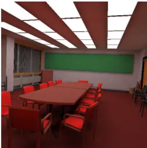
• Conference : a conference room with high geometric com-plexity (90 000 triangles)
• Cabin : a scene with many rooms (45 000 triangles)
Scene PT NS PS1 PS2 IR
Caustics 0.91s 178901 1.06s 2.48s 0.4s
Conference 9.13s 160516 1.23s 3.06s 1.8s
Cabin 4.76s 187184 1.17s 2.57s 1.2s
Table 1: Comparison with three scenes, PT : photon tracing, NS : number of splats, PS1 : photon splatting for a 512x512 image and PS2 : photon splatting for a 900x900 image , IR : image reconstruc-tion
All results were obtained with a 1.2GHz Athlon processor, 512 Mb of memory and a GeForce3 graphic card. First, results in Ta-ble 1 are presented for a coarse solution (100 000 photons traced from the light sources) using fixed bandwidth reconstruction. The results of the photon splatting pass seems slow compared to the specification of the graphic card. In opposition to first belief, the bottleneck is not only the frequent reading of the frame buffer. It is only responsible of one third of the rendering time even if there is ten to twelve reading of the frame buffer. We think the main bot-tleneck is the huge overdraw of the splats. Clearly, our method is fillrate limited.
Method 1e5 1e6 1e7
Fixed 1.23s 5.68s 15.06s
Adaptative 7.3s 14s3 39s
Table 2: Simulation on the Conference scene with different number of photons and the two methods
As expected, the scaling with scene complexity of the photon tracing pass is logarithmic. The increasing time with respect to the geometric complexity during the image reconstruction pass is due to the computation the intersection area between the kernel support and the surface. Otherwise, the splatting of the photons is totally scene complexity independent. It shows clearly that our method is scalable with scene complexity.
In Table 2, some results are shown with the Conference scene but with different accuracy for the light transport pass. The time of
adaptive reconstruction are given for a maximum of four decreasing bandwidth. These results shows that the complexity of the recon-struction pass does not depend only on the number of splats and the size of image but also depends on the average size of the splats in the image. It is shown in Table 2 because between a simulation with 100 000 photons and one million, there is tenth more splats but the increase in time of the reconstruction is much lower. Also, the sim-ulation with 10 millions of photons uses disk caching. It explains the relative increase in time. Disk caching is done directly by our software. Because the photons are accessed linearly, it is very easy to implement. In that case, the photons are stored in only 64MB to test the efficiency of disk caching.
7
Conclusion
In this paper, we have presented a two pass method to compute an irradiance image of a scene. The image can be recomputed ef-ficiently for different viewpoints. Our method has several advan-tages. First it is very scalable with respect to the geometric com-plexity. The photon tracing pass has logarithmic complexity and the reconstruction does not depend strongly on the geometric com-plexity. Another advantages is that our algorithm uses computer resources often neglected by other global illumination algorithms : graphics card and hard drive storage. Our method will certainly takes advantage of the increasing computational power of graphics hardware. Moreover, next generation of consumer card will sup-port more precision for the frame buffer which is positive for the accuracy of our algorithm. On the other hand, our method is fill-rate limited, so using a higher precision buffer will also decrease efficiency.
Also, we plan to integrate photon splatting in a more general global illumination algorithm. Indeed, to integrate effect as specu-lar reflections and refractions, photon splatting can be used with a ray tracer. Particuraly, image based ray tracer [Lischinski and Rap-poport 1998] seems a promising approach to compute the full light transport paths.
Figure 7: Conference scene with 1 million of photons and adaptive reconstruction.
References
CHEN, S. E., RUSHMEIER, H. E., MILLER, G., ANDTURNER,
Illumi-nation. In Computer Graphics (ACM SIGGRAPH ’91
Proceed-ings), vol. 25, 164–174.
CHRISTENSEN, P. H. 1999. Faster photon map global illumination.
Journal of Graphics Tools 4, 3, 1–10.
GRANIER, X., DRETTAKIS, G., ANDWALTER, B. 2000. Fast
global illumination including specular effects. In Rendering
Techniques 2000 (Proceedings of the Eleventh Eurographics Workshop on Rendering), Springer Wien, New York, NY, B.
Pe-roche and H. Rushmeier, Eds., 47–58.
HECKBERT, P. 1990. Adaptive Radiosity Textures for Bidirec-tional Ray Tracing. In Computer Graphics (ACM SIGGRAPH
’90 Proceedings), vol. 24, 145–154.
JENSEN, H. W. 1996. Global Illumination Using Photon Maps. In Rendering Techniques ’96 (Proceedings of the Seventh
Euro-graphics Workshop on Rendering), Springer-Verlag/Wien, New
York, NY, 21–30.
KAJIYA, J. T. 1986. The Rendering Equation. In Computer
Graph-ics (ACM SIGGRAPH ’86 Proceedings), vol. 20, 143–150.
LISCHINSKI, D., ANDRAPPOPORT, A. 1998. Image-based
ren-dering for non-diffuse synthetic scenes. In Renren-dering Techniques
’98 (Proceedings of the Ninth Eurographics Workshop on Ren-dering), 301–314.
MYSZKOWSKI, K. 1997. Lighting reconstruction using fast and adaptive density estimation techniques. In Rendering
Tech-niques ’97 (Proceedings of the Eighth Eurographics Workshop on Rendering), Springer Wien, New York, NY, J. Dorsey and
P. Slusallek, Eds., 251–262. ISBN 3-211-83001-4.
SHIRLEY, P., WADE, B., HUBBARD, P. M., ZARESKI, D., WAL-TER, B., AND GREENBERG, D. P. 1995. Global Illumina-tion via Density EstimaIllumina-tion. In Rendering Techniques ’95
(Pro-ceedings of the Sixth Eurographics Workshop on Rendering),
Springer-Verlag, New York, NY, P. M. Hanrahan and W. Pur-gathofer, Eds., 219–230.
SILVERMAN, B. 1986. Density estimation for statistics and data
analysis. Chapman and Hall, New York NY.
STURZLINGER, W.,ANDBASTOS, R. 1997. Interactive
render-ing of globally illuminated glossy scenes. In Renderrender-ing
Tech-niques ’97 (Proceedings of the Eighth Eurographics Workshop on Rendering), Springer Wien, New York, NY, J. Dorsey and
P. Slusallek, Eds., 93–102. ISBN 3-211-83001-4.
SUYKENS, F.,ANDWILLEMS, Y. D. 2000. Density control for
photon maps. In Rendering Techniques 2000 (Proceedings of the
Eleventh Eurographics Workshop on Rendering), Springer Wien,
New York, NY, B. Peroche and H. Rushmeier, Eds., 23–34.
VEACH, E., AND GUIBAS, L. J. 1995. Optimally Combining
Sampling Techniques for Monte Carlo Rendering. In Computer
Graphics Proceedings, Annual Conference Series, 1995 (ACM SIGGRAPH ’95 Proceedings), 419–428.
VEACH, E., ANDGUIBAS, L. J. 1997. Metropolis light trans-port. In Computer Graphics (ACM SIGGRAPH ’97
Proceed-ings), vol. 31, 65–76.
WALTER, B. J. 1998. Density Estimation Techniques for Global
Il-lumination. PhD thesis, Program of Computer Graphics, Cornell
University, Ithaca, NY.
WARD, G. J.,ANDHECKBERT, P. 1992. Irradiance Gradients. In