1
Bénard instabilities in a binary-liquid layer evaporating into an inert gas
H. Machrafia,*, A. Rednikovb, P. Colinetb, PC. DaubyaaUniversité de Liège, Thermodynamique des Phénomènes Irréversibles, Institut de Physique B5a, Allée du 6 Août, 17, B-4000 Liège 1, Belgium
bUniversité Libre de Bruxelles, TIPs – Fluid Physics, CP165/67, Avenue F.D. Roosevelt, 50, B-1050 Bruxelles, Belgium
Abstract
A linear stability analysis is performed for a horizontal layer of a binary liquid of which solely the solute evaporates into an inert gas, the latter being assumed to be insoluble in the liquid. In particular, a water-ethanol system in contact with air is considered, with the evaporation of water being neglected (which can be justified for a certain humidity of the air). External constraints on the system are introduced by imposing fixed “ambient” mass fraction and temperature values at a certain effective distance above the free liquid-gas interface. The temperature is the same as at the bottom of the liquid layer, where, besides, a fixed mass fraction of the solute is presumed to be maintained. Proceeding from a (quasi-)stationary reference solution, neutral (monotonic) stability curves are calculated in terms of solutal/thermal Marangoni/Rayleigh numbers as functions of the wavenumber for different values of the ratio of the gas and liquid layer thicknesses. The results are also presented in terms of the critical values of the liquid layer thickness as a function of the thickness of the gas layer. The solutal and thermal Rayleigh and Marangoni effects are compared to one another. For a water-ethanol mixture of 10 wt% ethanol, it appears that the solutal Marangoni effect is by far the most important instability mechanism. Furthermore, its global action can be described within a Pearson-like model, with an appropriately defined Biot number depending on the wavenumber. On the other hand, it is also shown that, if taken into account, water evaporation has only minor quantitative consequences upon the results for this predominant, solutal Marangoni mechanism.
Keywords
Stability analysis, binary mixture, evaporation, Rayleigh, Marangoni, solutal and thermal effects 1. Introduction
In standard studies [1-8] of convective instabilities of horizontal fluid layers, the destabilizing gradient across the layer is directly controlled from the outside of the system, through boundary conditions below and above the layer. The instability due to gravity and density variations is usually called Rayleigh-Bénard instability, while Marangoni-Bénard instability refers to the case where the surface tension variations are the driving factor behind it. When both effects couple, the term “Rayleigh-Marangoni-Bénard instability” is used. If it is the concentration dependence of the density and surface tension that causes the onset of convection, the corresponding instabilities can be called “solutal” Rayleigh-Marangoni-Bénard instabilities. Likewise, “thermal” instabilities result from the similar role of the temperature.
When evaporation takes place at the upper surface of the liquid layer, the situation becomes even more intricate. Indeed, evaporation is an endothermic process, resulting into the cooling of the liquid surface. In the case of binary mixtures, it is also accompanied by concentration gradients across the layer. Since the density and surface tension depend on both the temperature and the concentration, evaporation can thus indirectly destabilize the liquid layer.
Convection due to evaporation is an important phenomenon that occurs in many applications, such as during the drying of paint films, coatings, heat exchangers and process engineering installations. It also occurs in nature when for instance a salty lake dries out due to the evaporation of water, leaving behind structures on the soil. Several theoretical works have already been published on evaporation-driven Bénard instability of a one-component liquid layer [9-15], with the liquid evaporating in either an inert gas [9-13] or in its own vapor [6, 14-15]. To our knowledge, the studies of two-component systems has been rather limited in this context. One can mention a scaling analysis [16] or experiments [17]. From the theoretical viewpoint, quite a comprehensive study has been carried out in the case of a spherical geometry, when the Marangoni (both thermal and solutal) instability has been considered for an evaporating binary-liquid droplet [18]. Let us also mention experiments in a Hele-Shaw cell configuration with evaporating water-alochol solutions [19,20], where density-fingering (plume-like) patterns have been observed after a certain time had elapsed since the exposure of the solution to the air, which is clearly a manifestation of a buoyancy-driven mechanism. Cellular Marangoni patterns have also been observed [19], which are then suppressed by adding a surfactant, and the theoretical
part of [19] concerns just the buoyancy-driven instability.
In the present paper, the Rayleigh-Marangoni-Bénard instability induced by evaporation is studied by means of a linear stability analysis in the case of a binary liquid layer, when both the solutal and the thermal factors are involved. The particular model used here assumes a dilute solution of which only the solute evaporates (even though the latter limitation is relaxed at a later stage). In this case, the gas layer consists of an inert gas and the vapor of the evaporating liquid. The aim of the paper is to study the different instability mechanisms and to assess the degree of their mutual importance using a configuration as simple as possible. A concrete example followed throughout the paper is a 10/90 wt% ethanol/water mixture at normal conditions.
The paper is organized as follows. In section 2, the studied configuration is described, and a mathematical formulation of the problem is provided assuming that it is only the solute (ethanol) that evaporates from the binary mixture. The reference state is considered in section 3. Section 4 is concerned with the formulation of the linear stability problem. The results of the linear stability analysis are presented in section 5, and the relative importance of various instability mechanisms is assessed. An approximate analytical treatment of the reference profile and of the marginal stability conditions (by means of a Pearson-like model) is carried out in section 6,
making use of various simplifications possible within the full model. In section 7, the model is generalized to account for solvent (water) volatility, although the analysis is limited to the approximate approach framework of section 6. Finally, the conclusions are summarized in section 8.
2. Description of the problem
The system the instability of which is studied in this paper is presented in Fig. 1. It consists of a binary liquid layer (thickness , also denoted , see the distinction between the two below) in contact with a gas layer (thickness , also denoted , so that is the total thickness of the two-layer system). The liquid layer rests on a horizontal solid surface with a fixed temperature. The liquid-gas interface is assumed to be undeformable. The liquid layer is made up of a solute in dilute concentration and a solvent. The gas layer consists of air (the absorption of which in the liquid is neglected) and the vapors of the solute and the solvent.
Binary liquid
Air, solute vapour +
solvent vapour
Evaporation
Bottom boundary; zd= 0 Interface; zd= hd Top boundary; zd= hd+ d gz
y
x
Fig. 1. Sketch of the studied system
The treatment of the gas layer adopted here follows Haut and Colinet [10]. The thickness in such an approach is just viewed as a semi-heuristic quantity describing the typical equivalent (effective) diffusion length in the gas phase as determined by external air currents which may be naturally present or deliberately created (ventilation) therein: is the distance at which the diffusion is formally of the same magnitude as the convective transport in a real setup. In this sense, the gas phase above this layer is considered as perfectly mixed while ensuring given “ambient” values of temperature (the same as at the bottom of the liquid layer in the case considered here) and concentration at the effective upper boundary of our gas layer. In this respect, the approach is actually rather similar to the so-called “stagnant film” approach, often used in chemical engineering [21]. The shear-induced influence of such currents on the liquid layer is neglected however, and thus no net horizontal flow in the gas phase is explicitly included into the model. Besides, the model is formulated assuming no externally imposed horizontal non-uniformities upon the system, implying that the scale of any horizontal non-uniformity that may exist in a real setup (as opposed to the present idealized configuration) is much greater than the
scale of the phenomena to be studied here (evaporation-induced Bénard instability). As for the hydrodynamic conditions at the effective upper boundary of the gas layer, we shall use the “soft” (“stress-free”) ones: no tangential stress and a given uniform pressure/normal stress. We note that, overall, despite its heuristic character, the proposed approach is more detailed and general than the frequently used one based upon describing the transport processes in the gas by means of simply a transfer coefficient (Biot number): the former permits to assess an active role of the gas phase in the studied phenomena, whereas the latter (being essentially a one-sided model of the liquid layer) does not.
The solvent is considered to be much less volatile than the solute. Actually, in the main body of the paper (sections 2-6), the solvent is formally treated as non-volatile. For a dilute solution of ethanol (solute) in water (solvent), which is a concrete example followed throughout the paper, such a treatment is expected to be approximately valid at some ambient humidity of the air, when the water vapor is nearly saturated relative to the solution (otherwise, even though water is indeed much less volatile than ethanol, its greater amount in the solution may make the effects of its evaporation nonetheless noticeable). At the end of the paper, however, we shall come back to the question of how the results change if water evaporation is incorporated into the model for an arbitrary humidity of the air.
Here we shall also assume that it is not only the temperature that is fixed at the bottom of the liquid layer, but also the concentration. While the latter assumption seems to be rather artificial, it will permit to study in a simple way (i.e. for a quasi-stationary reference state) the Bénard instability mechanisms pertinent to an evaporating binary-liquid layer and to assess their mutual importance, which is the main goal of th p se t papere re n .
Now a few words about the notations , , and as used here. Due to evaporation, the liquid thickness changes with time , which we describe here by introducing the function
. We can then define a constant quantity as the thickness of the liquid layer at a certain reference, or initial, time , i.e. 0 . This thickness will then be chosen as the unit length for non-dimensionalization. In dimensionless form, the bottom plate is located at 0, and the interface then corresponds to , with 0 1. Note that the
superscript “d” stands for the dimensional character a particular quantity, whenever it is used elsewhere in dimensionless form. Similarly, in view of the meaning attributed to the gas layer thickness here, (defined as the total thickness of the system) can in principle also be a function of time: . Then we define 0 0 for the initial thickness of the gas layer. In dimensionless form, the top of the gas phase corresponds to .
2.1 Bulk equations
The Boussinesq approximation [6] will be adopted for both phases of the system, implying that the material properties of the fluids are treated as constant except for the density in the buoyancy
terms, whose dependence on the temperature and mass fraction is taken in the following linearized form:
(1)
, 1 , , ,
, 1 , , , (2)
whereas the corresponding dependence on pressure is presumed to be negligible for the pressure range involved in the problem. Here, is the density, is the (dimensional) temperature, is the solute mass fraction, and are the thermal and the solutal expansion coefficients. The subscripts “l” and “g” relate to the liquid and gas phases, respectively. The subscript “0” refers to a certain reference state (to be specified later on). Clearly, the validity of different hypotheses underlying the Boussinesq approximation is limited to situations for which the temperature and mass fraction in the system remain close enough to the reference values introduced in (1) and (2).
As mentioned above, let be the length scale. The time scale is chosen as the liquid thermal time scale / . The dimensionless evaporation mass flux is obtained by using the scale
, where ,
is the evaporation number, is the temperature scale, is the heat of solution of the solute in the solvent, refers to the thermal diffusivity, the heat capacity and the thermal conductivity.
a the temperature scale such that We sh ll choose
, 1 .
However, we find it advantageous, for the sake of physical clarity of certain formulae, to keep the quantity unsubstituted, even though it will eventually be evaluated according to the above expression. The dimensionless temperatures and in the liquid and gas are respectively defined by , / and , / . The mass fractions are already dimensionless. The pressure and velocity scales are respectively chosen as and , where refers to the dynamic
s The following dimensionless balance equations are then obtained: visco ity. (3) · 0 , · 1 1 , 1 , (4) · , (5) · , (6) · 0 , (7) · ρ 1 ν 1 , 1 , (8) · κ , (9) · , (10)
where and are the (barycentric) velocity and pressure fields. For the liquid and gas phase respectively, (3) and (7) are the continuity equations for incompressible fluids, (4) and (8) are the momentum equations, (5) and (9) express the energy conservation, whereas (6) and (10) stand for the mass conservation of the solute species. The symbol
ψ
S accounts for the Soret effectnd is defined by (considered only in the liquid phase) a
, with , , , 1 , , (11)
where is the thermal diffusion coefficient and refers to the diffusion coefficient. , is the
Soret coefficient in the liquid (obtaining a value 0.154). In the gas phase, the Soret effect is neglected assuming small vapor concentration, in which limit this effect tends to disappear (and the same goes for the Dufour effect). Equations (3) through (10) contain the following
s n s u bers: dimen io les n m
, , , , , , , , ,
, ,
where refers to the kinematic viscosity and , , , and are respectively the Prandtl, Lewis, Galileo, thermal Rayleigh and solutal Rayleigh numbers in the liquid. The symbols , , , , and , without subscripts, denote the ratios of the corresponding material properties in the gas to those in the liquid.
For the subsequent discussions in the paper, it is also interesting to recall the following detailed imensionless expressions of the solute m ss and heat fluxes in the liquid and in the gas
), (9) a
d a
compatible with (5), (6 nd (10):
, , . (12)
Note that the scales used for the mass fluxes are the same as the one defined above for the evaporation flux (with 1). For the heat flux, the scale used is .
2.2 Boundary conditions
The fol boundar ns are a
0, , , (13)
lowing y conditio ssumed at the bottom of the liquid layer ( 0):
where and are some fixed values. Note that the boundary condition on the mass fraction is probably not easy to realize in practice. In principle, this condition could be realized by installing at the bottom a thin layer of a porous gel (of vanishing mass transfer resistance), under which a mixture of the solvent and the solute, with a fixed mass fraction , is circulated. In the present paper, as it has already been mentioned, we shall rather regard the third condition (13) as a model permitting to study in a simple way the basic instability mechanisms in a binary-liquid layer. In particular, it will allow consideration of a (quasi-)steady reference state (which would not be the case should a zero flux condition 0 be specified instead).
The boundary conditions to be specified at the top of the gas layer have in fact been already discussed when introducing the basic configuration. We have fixed constant values of the temperature and concentration, and , respectively, and the “soft” hydrodynamic conditions with the normal stress being equal to a certain value (an “external pressure”) and the
zero (“s f t s,
tangential stress being tress ree condi ion”). Thu ,
, 0, 2 , (14)
at , where
is the ratio of the dynamic viscosities. The symbols , and stand for the , and velocity field components, respectively. It will be seen that the form of the hydrodynamic conditions has little influence in practice (see subsection 5.7).
Consider now the conditions at the liquid-gas interface. Since evaporation takes place at this interface, the liquid layer thickness changes with time, but we assume that the interface remains flat. Note that this assumption will be discussed briefly at the end of section 6.2. Due to mass conservation, the evaporation flux is linked to velocities in both the gas phase and the liquid
moving with the interface . In our notations, this reads [6]
phase in the reference frame
, (15)
t (15) can also be solved with respect to and / to yield at . Note tha
, (16)
at .
(17)
Other boundary conditions at the interface express the continuity of the temperature and of the locity com o s : tan p nent , , (18) gential ve , at .
The energy conservation at the interface implies a balance between the heat fluxes in both phases h vaporation, which reads [6]
and t e heat of e
(19)
at , where
.
Note that the mechanical effects (kinetic energy flux and work of surface tension forces) are neglected in (19).
In expressing the tangential stress balance at the interface, it is assumed that the surface tension between the liquid and the gas depends on the temperature and on the solute mass fraction in the
y an write
liquid. Similarl to (1) and (2), one c
, , (20)
with
and .
Then, the conditions expressing the tangential stress balance at are [6]
0 , (21)
0 , (22)
where
, C
D
are the thermal and solutal Marangoni numbers.
The assumption that it is only the solute that evaporates implies that the evaporation flux is a evaporation flux of the solute only. The latter can be expressed as:
equ l to the
· 1 .
d using (12), one arrives at the following boundary condition at : By equating this to an
. (23)
The inert gas adsorption in the liquid is also neglected. Using an argument similar to the one ), one obtains the following additional boundary condition at :
leading to (23
. (24) A local equilibrium hypothesis at the surface is made to describe the evaporation process.
te binary liquid, it amounts to the so-called Henry’s law [22]: Assum g a di
,
in lu
where and are the molar fractions of the solute in the gas and liquid phases, respectively, and is the Henry coefficient (in pressure units), which generally depends on the interface temperature, even though this dependence is neglected in the present paper (this point will be justified a posteriori in Section 3, in the case of the reference solution). The quantity is the total pressure of the gas at the interface. In terms of mass fractions, Henry’s law can be rewritten as
, (25)
yielding another boundary condition at . The symbol stands for the dimensionless Henry coefficient (using / as the pressure scale). The symbol refers to the ratio of solvent and solute properties, the subscript of indicating the property in question. In (25)
is the solvent to solute molecular mass ratio, while
is the same for the air and the solute, where the subscript “a” refers to the air. Note also the notation
/
which will be used later on.
2.3 Comments on the linear stability analysis
The goal here is to examine the stability of the horizontally uniform solutions of the above equations, depending only on the vertical coordinate and characterized by zero horizontal velocity (the “reference” solutions). It should be realized, however, that due to the evaporation process at the liquid-gas interface, the thickness of the liquid layer will vary in the course of time. Consequently, the possible horizontally uniform solutions will be intrinsically time-dependent. However, the analysis is carried out assuming this variation to be slow enough (the quasi-stationary hypothesis, to be defined shortly). As a first step of our work, we obtain the (quasi-stationary) reference solution. The second step will consist in analyzing the stability of the reference solution. Since the latter depends on time, it must of course be understood that the stability analysis must be carried out as a function of time. This is accomplished in the framework of the frozen-time approach (also used in [23]), which is in any way nearly rigorous here on account of the mentioned quasi-stationary hypothesis (with the exception of certain modes as discussed later on).
More precisely, the quasi-stationary assumption consists in assuming that the liquid thickness varies sufficiently slowly for the temperature, mass fraction and velocity profiles in both phases to reach a steady state corresponding to an instantaneous value of . In other words, this hypothesis amounts to the assumption that the time scale of the variations of is much larger than the diffusive time scales of the problem. To determine the quasi-stationary reference solution, all time derivatives in the equations can be cancelled, except for the time derivative of in (16). It goes without saying that this ansatz is not valid for very short times, when the diffusional profiles have not yet invaded the whole layer. As a consequence of this
quasi-stationary assumption and the corresponding separation of timescales, it is easy to understand that among all the unknowns of the problem, only will explicitly depend on time, following (16), while all other quantities of the reference solution will depend on only through itself. Note that this provides the reason why the approach is called quasi-stationary. As a further interesting consequence of this hypothesis, one can understand that performing a frozen-time stability analysis of the reference solution for all frozen-times is completely equivalent to performing the stability analysis for all possible values of . Switching to this point of view amounts to asking for what an instability can occur, instead of asking for what time this
instability appears, which is often more interesting from a physical point of view and which will actually be done in the following.
In the framework of this approach, the time introduced above can be chosen, without loss of generality, as the time corresponding to the thickness 0 for which the stability analysis shall ormed. Following the procedure described before, to non-dimensionalize the equations,
uces that the dimensionless liquid thickness can be set to unity be perf
one ded 1.
Note that this result does not imply that the dimensionless thickness is fixed, but only means that its value, at the time for which a stability analysis will be carried out, is equal to unity. Let us also stress that replacing the dimensionless liquid thickness by unity is a bit delicate, since this amounts to hide that the reference solution indirectly depends on time through and to transfer this time dependence in the length scale used to non-dimensionalize the equations. Fortunately, this will not prevent a proper stability analysis, as we will explain later.
In principle, in accordance with the approach used for the gas layer in our system, as set forth in the beginning of section 2, can also be a function of time. Furthermore, unlike whose time dependence is embedded into the formulation by means of (16), for , it is largely controlled by the external constraints on the system which remain outside the present formulation. For instance, for constant external constraints, it may be reasonable to assume that it is
(the dimensional gas layer thickness) that remains constant, but then will evolve together with . In any event, the time dependence of (if any) will be presumed as slow as that of .
2.4 Water-ethanol system and external constraints
Before undertaking the stability analysis, it is important to stress that a very large number of parameters appear in the equations presented above and that it is not feasible to carry out a general parametric study. For this reason, we shall first restrict our analysis to a water-ethanol liquid layer, with only ethanol evaporating into air. Then, we shall assume that the temperatures imposed at the bottom and at the top of the system are equal. In this way, any thermal instabilities that may appear in the system would result exclusively from the evaporation process. The reference temperatures in both the liquid and the gas phases that are used in (1), (2) and (20) are then fixed at this value, i.e. , , . This means that we have just 0 in dimensionless form.
We shall also choose the mass fraction imposed at the bottom of the system as the typical concentration , , introduced in (1), (11) and (20). Similarly, the concentration imposed at the top of the system is used as the typical concentration , introduced in (2). The value must be small enough for Henry’s law, corresponding to dilute solutions, to be actually valid. In particular, the following values are chosen: 300 , 0. For the mass fraction imposed at the bottom, two different values are considered in our results, namely 0.1 and
0.001. The different thermo-physical properties of the liquid used in the calculations are those corresponding to the reference values of the temperature and composition imposed at the bottom of the system. Similarly, in the gas, the thermo-physical properties correspond to the reference temperature and composition imposed at the top of the upper layer. When needed, the properties are also determined for a value of the pressure equal to the atmospheric pressure
1 atm.
The numerical values of the physical properties are given in tables 1 and 2, and for the interested reader, Appendix A presents some details on how these values have been obtained.
Table 1. Physical properties of the gas layer Physical property Value
1.18 kg/m3 , 1.005*103 J/kg K 2.62*10-2 W/m K 2.22*10-5 m2/s 1.58*10-5 m2/s 1.85*10-5 Pa*s 3.35*10-3 K-1 1.20*10-5 m2/s -3.70*10-1
Table 2. Physical properties of the liquid layer
Physical p perty ro Value for = 0.1 Value for = 0.001 9.796*102 kg/m3 9.964*102 kg/m3 , 4.26*103 J/kg K 4.18*103 J/kg K 5.31*10-1 W/m K 6.07*10-1 W/m K 1.27*10-7 m2/s 1.46*10-7 m2/s 1.33*10-6 m2/s 8.5*10-7 m2/s 1.3*10-3 Pa*s 8.5*10-4 Pa*s 3.4*10-4 K-1 2.75*10-4 K-1 1.0*10-9 m2/s 1.3*10-9 m2/s 1.53*10-1 1.92*10-1 1.45*10-4 N/m K 1.6*10-4 N/m K 1.4*10-1 N/m 5.0*10-1N/m , / 3.26*10-1 atm 3.26*10-1 atm 1.13*106 J/kg 1.13*106 J/kg 6.46*10-3 K-1 7.58*10-3 K-1
3. The reference state
In the present section, we will determine the reference solution, the stability of which will be examined later on. We shall do it in the framework of the quasi-stationary assumption as discussed in subsection 2.3.
In seeking the reference solution, the partial time derivatives are neglected in the balance equations (3)-(10). When the horizontal derivatives are also disregarded, one obtains a system of ordinary differential equations with respect to the vertical coordinate . Using the boundary conditions at 0, 1 and , these equations can be solved, as now explained.
The first of the boundary conditions (13) together with the incompressibility assumption (3) lds the reference solution for the velocity in the liquid phase:
directly yie
0 . (26)
,
Simila ly, equa
, 1
r tions (7) and (17) yield
, (27)
w ereas n
(28)
h ote that
according to (16). Using (5), the second of Eqs (13) and Eq. (26) yields the following reference uid phase:
solution for the temperature in the liq
, , (29)
,
where the subscript “i” refers to the interface, and where the reference interfacial temperature
w e d tion (9) and the first condition (14) yield
, ill b etermined below. Similarly, equa
, , ,
, /
, / . (30)
Proceeding similarly for the mass fractions, by using (6), (10), the third of Eqs (13) and the
( o tains
second of Eqs 14), one b
, , , (31)
,
, , , , ,
, /
, / . (32) In what follows, we will also need the pressure field in the gas in order to use it in Henry’s law. From (8) together with (30), (32) and the last equation (14), one obtains the gas pressure distribution in the reference state, , . In particular, its value at the interface ( 1) is found to be , , 1 , , , / , , , / , , , , , . (33)
In (29), (30) and (33), and denote respectively the temperature at the bottom and top plates. These are equal to one another as stipulated earlier (cf. subsection 2.4) and moreover
0, but in order to trace back the place of each quantity in the formulae, the symbols are left as such. The mass fractions and in (31) and 32) are also considered as known constants. ( The four constants , , , ,, , , and introduced above still need to be calculated in
order to completely determine the reference solution. The equations they obey are derived from conditions (19) and (23)-(25) upon the substitution of (26)-(33) therein. One obtains the following system of four equations:
, , , (34) , / , , , , , (35) , , 1 , , , , / , , (36) , , , , , , , , , , . (37)
This non-linear system (34)-(37) must be solved numerically for the four unknown constants, which results in a complete determination of the quasi-stationary reference solution. As illustrations, some of the reference temperature and mass fraction profiles are presented in Figs. 2 and 3 for the water-ethanol system with = 0.1 for several values of . Typical numerical values of some parameters are also given in Table 3. Let us also mention that a detailed analysis of the solutions obtained (which is actually not presented here) shows that the pressure does not change significantly across the system. Indeed, for values of between 1.5 to 101, and for
1 atm, it appears that , , is always smaller than 1 Pa. Finally, note also that, as announced in section 2.3, equation (16) was not used to determine the solution given above. In case one is interested in the variation of with time, the above calculations must be repeated for 1 and (16) can then be used as a (non-linear) ODE for . Remark the weak deviations of the temperature with respect to 300 K, in Fig. 2, which justifies our hypothesis to neglect the variations of the Henry constant (and, in principle, of other physical properties) with the temperature. Note from Fig. 3 that the mass fraction in the gas is an order of magnitude smaller than that in the liquid, which justifies the hypothesis to neglect the Soret effect in the gas phase.
0 0.5 1 1.5 2 2.5 3 3.5 4 299.82 299.85 299.88 299.91 299.94 299.97 300 z‐ coo rdi n a te T [K] T Fig. 2. Temperature distribution in the reference state (10 wt% ethanol in water)
Fig. 3. Solute mass distribution in the reference state (10 wt% ethanol in water)
In the previous text, the quasi-stationary assumption has been used. It is interesting to investigate to what extent this assumption is valid (excluding very short times as mentioned in section 2.3). This can be done by examining the relevant time scales. For the liquid phase, the time scales in question are the time scale for the variation of the liquid height ( / ), the diffusion time scale ( / ), the thermal time scale / and the viscous time scale / . The first of them must be much larger than the other three for the quasi-stationary assumption to hold. The corresponding ratios give rise to the diffusion and thermal Péclet and Reynolds numbers that must be small. As typically and , it is the diffusion Péclet number in the liquid
l,ref Tg,ref Tl,ref Tg,r f H = 2 H = 1.5 H = 4 e 0 0.5 1 1.5 2 2.5 3 3.5 4 0 0.01 0.02 0.03 0.04 0.05 0.06 0.07 0.08 0.09 0.1 z‐ coo rdi n a te Mass fraction of the solute Cl,ref Cg,ref H = 1.5 H = 2 H = 4 H = 4 H = 2 H = 1.5 cl,ref cg,ref
,
,
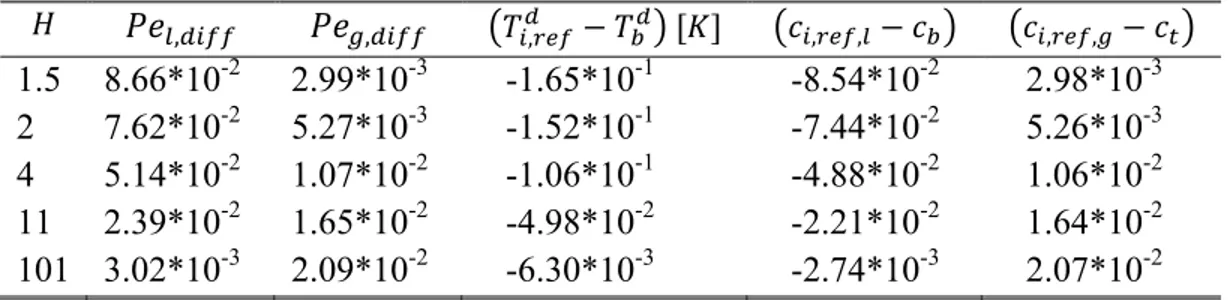
(with various equivalent expressions provided) that must be followed as the criterion of quasi-stationarity ( , 1). Its values are shown in dimensionless form in Table 3 for a number of cases and turn out to be small indeed: the more so, the bigger is. Note that the concentration gradient in the liquid turns out to be of the order , .
From the gas side, the corresponding criterion of quasi-stationarity is / 1 . As 1, which brings about | | , (cf. (27) and (28)), the dimensionless number /
aller than what we shall call the Péclet number in the gas: is anyway much sm
, , / .
Thus, should it be that , 1, then the quasi-stationarity criterion in the gas is satisfied all the more. On the other hand, , is the criterion of non-linearity of the profiles (30) and (32) with respect to . , indeed happens to be small in our example, as substantiated by its values represented in Table 3, which explains why the profiles in the gas phase shown in Figs. 2 and 3 are almost linear, and at the same time justifies the quasi-stationary assumption Another interesting observation from Table 3 is that , happens to be nearly equal to ( , , ), the two being small. Note that in the work [18], devoted to the Marangoni instability in an evaporating binary-liquid droplet, the same type of criteria have been elaborated to validate the quasi-stationary assumption. Their calculations showed as well that the gas phase could be treated as asymptotically steady and that the regression of the surface was negligible.
Table 3. Numerical values of some quantities in the reference solution for different values of H ( wt%10 ethanol in w , ater) , , , , , , 1.5 8.66*10-2 2.99*10-3 -1.65*10-1 -8.54*10-2 2.98*10-3 2 7.62*10-2 5.27*10-3 -1.52*10-1 -7.44*10-2 5.26*10-3 4 5.14*10-2 1.07*10-2 -1.06*10-1 -4.88*10-2 1.06*10-2 11 2.39*10-2 1.65*10-2 -4.98*10-2 -2.21*10-2 1.64*10-2 101 3.02*10-3 2.09*10-2 -6.30*10-3 -2.74*10-3 2.07*10-2
Table 3 also shows that for increasing , the mass fraction gradient in the liquid phase gets smaller and smaller ( , , ), which provides a justification for not considering in our model the variation of the material properties with the concentration in the liquid phase, even if some of them (for instance, the diffusion coefficient [24], the Soret coefficient (11) or ) are rather sensitive to . Note that one can also make use of the smallness of the Péclet numbers, and of some other effects, in order to build an approximate model of the stability problem, as we will show later in section 6. Also provided in Table 3 are the numerical values of the temperature gradient for possible comparison by other readers.
4. Stability of the reference solution
In order to study the stability of the reference solution, the time evolution of small perturbations with respect to this solution must be studied. These perturbations are introduced by expressing
the unknowns as ′, ′, ′, ′, ′.
Following a standard procedure, these decompositions can be introduced in the bulk equations and boundary conditions, which are then linearized with respect to the infinitesimal perturbations. As far as the liquid-gas interface is concerned, it is important to stress that the corresponding boundary conditions must be expressed at ′ and linearized with
respect to h’. Note that in the following the primes, denoting the perturbations of the reference state, will be omitted for simplicity.
The stability analysis is carried out in the framework of the so-called “frozen-time” approach, i.e. the evolution of perturbations is calculated in the form of normal modes superposed to each instantaneous snapshot of a time-evolving reference profile, as if the latter wasere stationary. On account of the quasi-stationarity assumption adopted in the present paper (see subsection 2.3), the frozen-time normal-mode approach tends to become exact: the smaller the Péclet numbers (see previous section), the more so. Of course, this tacitly implies that the perturbations evolve on the time scale of diffusion in the liquid at the slowest, which will actually be the case for all the modes but one considered hereafter. This exceptional mode will be a slow one, associated with the time evolution of the liquid layer thickness, for which the frozen-time approach bears all its “standard” shortcomings. Under the undeformable surface assumption used here throughout, it will be just an isolated mode corresponding to a zero wavenumber. For the sake of concreteness, we shall treat it here assuming that it is only the thickness of the liquid layer that is perturbed, and not the total thickness of the two layers (i.e. the perturbation of is equal to zero), even though other arrangements are in principle possible within the conceptual framework set forth in the beginning of section 2.
The horizontal components of the velocity can be eliminated from the equations as usual (by applying to the momentum equation). The normal modes are introduced as follows:
, (38)
, (39)
In (38)-(40), σ is the complex growth rate of the perturbations and , is the wavevector (with the wavenumber ), whereas W,
θ
, C and P are the complex amplitudes (functions of z). In (40), the vanishing of for non-zero wave vectors is a consequence of the assumption of an undeformable liquid-gas interface. Note that does not depend on , of course.The (linear) equations for the amplitude of the perturbations, as derived from (3)-(10) and valid for both zero and non-zero wavenumber, are found to be
, (41) (42) , , (43) , , , , (44) , (45) , , , , , . (46)
Later on, we will eventually need the following expression for the pressure amplitude in the gas phase, which is easily deduced starting from the perturbed form of (7) and the horizontal
component of (8):
, . (47)
The boundary conditions are derived from (13), (14), (15)-(19) and (21)-(25). At 0, one obtains
0, 0 , 0. (48)
0,
, th ary con n e litudes of the perturbations write At e bound ditio s for th amp
0, 0, 0 , 2 0. (49) As said above, the condi ns the moving interface 1 are linearized with respect to
ns. One obtains the following relations at 1: tio at
and with respect to all perturbatio
(50) , 0 , 0, 0 , , 0 (52) , (51) , 0 0 , 2 2 0 , (53) , , , , , , (54) , , , , , (55)
, ,
, ,
, ,
, , ,
, , (56)
with given by (47) and with 0 if 0. Here we have also taken into account (26) and that , 0 in accordance with (27).
Thus, an eigenvalue problem for the growth rate of perturbations has been obtained, the results for which are analyzed below.
5. Linear sta ility results b In the case
5.1 Numerical results for the non-zero mode case
0, the eigenvalue problem presented above is solved using a Tau-Chebyshev method, which is rather classical and thus not recalled here (see for instance [25,26]). Before proceeding to the results, let us stress that in the classical studies of the Rayleigh-Marangoni problems, the control parameter is just the imposed temperature gradient. In the present case of evaporation, we assume so that the resulting temperature gradients are a consequence of the evaporation process, which is controlled by above the gas not being in equilibrium (in the sense of Henry’s law) with at the bottom of the liquid. Here, we shall take 0 and study two different values of . With these boundary conditions and with clearly defined components in the liquid and gas phases (water, ethanol and air), the main control parameters we are left with are just the thicknesses of the liquid and gas layers, and . In principle, the background temperature also plays a role as the material properties (and perhaps most notably the Henry coefficient) depend on it. An imposed pressure could also be used to control the mass fraction in the gas phase (and influence the mass fraction in the liquid phase by Henry’s law). However, the two latter types of control are not considered in the present paper. The control parameters ( and ) enter into the dimensionless formulation by means of the dimensionless numbers , , , , and . Varying and means varying these numbers, albeit not independently once the system and the constraints have been fixed physico-chemically. The marginal stability curves are obtained by calculating, as a function of the wavenumber , the value of the liquid layer thickness for which the condition Re 0 (vanishing of the largest real part of all growth rates) holds, keeping all the other parameters fixed. First let us mention that the instability is always monotonic, since our numerical results show that Im is always equal to 0 for the marginal states. Fig. 4(a) presents the neutral curves corresponding to 2, 11 and 101. Fig. 4(b) is a plot of the critical wavenumber as a function of and shows that this critical wavenumber remains approximately constant and close to 2 over the whole range of values of .
(a) (b)
Fig. 4. Neutral stability curve in terms of the liquid layer thickness for 2, 11 and 101 (10 wt% ethanol in water) 0.01 0.10 1.00 10.00 0 1 2 3 4 5 dl [1 0 ‐6m] k H=2 H=11 H=101 0 0.5 1 1.5 2 2.5 3 0 20 40 60 80 100 1 H 20 kc = kc dd l
To examine the influence of the gas layer thickness (dg) on the stability threshold, we have
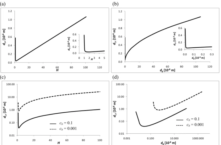
plotted in Fig. 5 the critical liquid thickness (i.e. the minimum of the neutral stability curve of Fig. 4) as a function of H , and also as a function of dg. Figs. 5(a) and 5(b) correspond to = 0.1.
In Fig. 5(c) and (d), the results for = 0.001 are also shown for comparison. (a) (b) 0.0 0.2 0.4 0.6 0.8 1.0 1.2 0 20 40 60 80 100 120 dl,c [10 ‐6m] H 0.0 0.2 0.4 0.6 0 1 2 3 4 5 dl,c [1 0 ‐6 m] H 0.0 0.2 0.4 0.6 0.8 1.0 1.2 0 20 40 60 80 100 120 dl,c [1 0 ‐6m] d [10 m] (c) (d)
Fig. 5. The critical liquid thickness as a function of H (a) and dg (b) for an ethanol/water system
with = 0.1 (10 wt% ethanol in water), and the same, albeit in different scales, together with the results for = 0.001 (0.1 wt% ethanol in water) (c, d)
g ‐6 0.0 0.2 0.4 0.6 0.0 0.1 0.2 0.3 dl,c [1 0 ‐6m] dg[10‐6m] 0.01 0.10 1.00 10.00 100.00 0 20 40 60 80 100 dl,c [10 ‐6 m] H Cb = 0.1 Cb = 0.001 0.01 0.10 1.00 10.00 100.00 0.001 0.100 10.000 1000.000 dl,c [10 ‐6m] d [1 Cb = 0.1 C g 0‐6m] b = 0.001 cb = 0.1 cb = 0.001 cb = 0.1 cb = 0.001 H = 2 H = 11 H = 101
Fig. 5(a), corresponding to = 0.1, shows that there is a linear relation between the critical thickness and H for sufficiently large values of H (practically, higher than 2). This corresponds to a scaling , ~ . for large , which is indeed observed in Fig. 5(b). Note also that for very thin gas layers (Fig. 5(b)), the critical liquid height increases very sharply and diverges to infinity, leaving a certain minimum in between. A physical interpretation of this minimum will be presented in section 6, in relation with Fig. 12. It can also be noted that the critical liquid heights are rather small. This means that liquid layers of reasonable thicknesses will be very unstable. This somehow confirms the scaling analysis performed in [16]. Note that the critical wavenumber for these results always appeared to be around 2. For = 0.001 (Figs. 5(c) and (d)), the same observations are made and the same trends are observed. The only difference is that the critical liquid thickness is roughly 25 times larger for = 0.001 than for = 0.1. The interest of using two different bottom mass fractions is to find out whether a very dilute liquid produces different results. It is clearly shown that the decrease of the solute concentration has a stabilizing effect. One should remember, however, that the results for = 0.001 are obtained while neglecting the evaporation of water (which is a strong limitation for so small concentrations).
5.2 Numerical results for the zero wavenumber case
The solution of the eigenvalue problem for 0 does not require the use of the Tau-Chebyshev method. First, a closed form solution can be obtained easily for the perturbations W,
θ
and C [27] leaving some unknown constants (including the growth rate and the amplitude of the liquid thickness perturbation). Then these unknown constants can be numerically determined by solving the non-linear algebraic equations provided by the boundary conditions (50), (51), the second condition (52), (54)-(56) and a normalization condition for the solution. In particular, an infinite numbers of growth rates can be numerically determined for any fixed value of H. In the zero-mode case, these growth rates do not depend on and and depend on the dimensionless numbers and only via the reference pressure in the gas phase. Here, though, this dependence is so weak (pi,ref,g – pt < 1 Pa) that it can be neglected. Therefore, thegrowth rates depend significantly on the control parameters ( and ) only via the value of . The results of these calculations can be summarized as follows. For any given H, all the calculated growth rates have negative real parts, except one which is real and positive. The latter is not unexpected and indicates that the evaporation rate increases with the decrease of the liquid layer thickness, which within the frozen-time approach boils down to this positive growth rate. Note also that this positive value appears to be much smaller than the absolute value of the real parts of all other values of the growth rate. Since (note the different meaning of this quantity as compared to the one used in section 3, since in this case it concerns the perturbations and not the reference state), the smallness of the positive growth rate expresses once again that
the characteristic time of the variation of the depth of the liquid is much longer than the other time scales in the problem.
As a consequence of the above discussion, we can conclude that no mode with 0 is able to destabilize the reference state unless on a very long time scale, comparable to the time it takes to fully evaporate the layer. In principle, all what concerns this mode would be best captured by relaxing the limitation of surface non-deformability used in the present paper and developing a lubrication-approximation (non-linear) theory of an evaporating liquid layer much along the lines of [28] (where a similar homogeneous mode has been identified). In the present paper, however, we shall rather be interested in an evaporation-induced Bénard convection appearing on a shorter time scale, whose existence is indicated by the linear stability analysis results of subsection 5.1.
5.3 Comparison of the solutal, thermal and Soret contributions to the Rayleigh and Marangoni effects
In the following subsections 5.3-5.6, we analyze in more detail the physical mechanisms responsible for the instability and we start here by comparing the thermal and solutal contributions, for both the Rayleigh and the Marangoni effects.
Consider first the Rayleigh effect and let us combine equations (41)-(43) for marginal perturbations 0 to deduce the following single equation for only:
, , , , . (57)
Three additive terms depending on gravity can be distinguished in (57). Accordingly, three contributions to the Rayleigh effects can then be identified and quantified. Two of them describe
l e lo ing dimensionless numbers: thermal and soluta ffects by the fol w
, ,
, , , ,
, (58)
, (59)
Th Soret e fect is then described by the llo
, ,
e f fo wing dimensionless number:
, .
can be defined as a “true” thermal Rayleigh number and accounts for the thermal Rayleigh effect. is the “true” solutal Rayleigh number and accounts for the solutal Rayleigh effect. The number is referred to as the “Soret Rayleigh number”. The latter number stands for the density effects that are solutal in nature ( ) but caused by thermodiffusion (Soret effect). In order to assess the relative importance of these effects with respect to one another, three ratios can be defined: the solutal and thermal effects can be compared by examining the number
/ , while the solutal and the Soret-Rayleigh effects are compared by considering the number / and the thermal effect and the Soret-Rayleigh effect can be compared using the number / .
The same evaluation can be done for the Marangoni effect, but unlike the Rayleigh case one can no longer derive a single relation where one could observe the relative importance of various contributions as clearly as in (57). However, a straightforward order-of-magnitude argument allows introducing “true” Marangoni numbers, whose definitions fully parallel those given for
ers. For the therma lutal effects, this gives
the Rayleigh numb l and so
, µ , ,
, , , ,
(60)
, (61)
For the Soret effect, this gives
, , , .
is the “true” thermal Marangoni number, with being the “true” solutal Marangoni number, while being referred to as the “Soret Marangoni number”. This number stands for the surface tension effects that are solutal in nature ( ) but caused by thermodiffusion. In the same manner as in the Rayleigh case, the comparison between the solutal effect and the thermal and Soret-Marangoni effects can be performed by considering the ratios / , / and fte all these ratios, one can first note that in fact two of them are equal, with / . A r defining
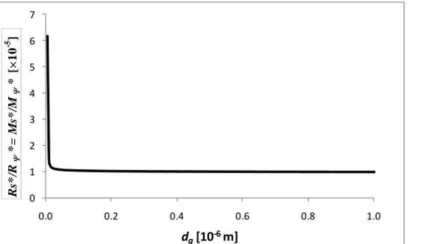
, , , , .
This number, calculated for a liquid thickness equal to its critical value (function of ), represents the relative importance of the solutal and Soret effects for both the Rayleigh and Marangoni cases. In Fig. 6, it is plotted as a function of the gas layer thickness (for the water-ethanol system, with = 0.1).
0 1 2 3 4 5 6 7 0.0 0.2 0.4 0.6 0.8 1.0 dg[10‐6 m] Rs * /R Ψ *= M s* /M Ψ * [× 1 0 -5 ]
Fig. 6. The ratios of the solutal and the Soret contributions as a function of dg (10 wt% ethanol in
water)
On th o er hand e th , the ratios of the thermal and the Soret contributions are given by: , 3.82 ,
Ψ ,0 1.78 , (62) where the estimations are made for the water-ethanol system ( = 0.1) and show that the two effects are of the same order of magnitude, although the thermal one is somewhat stronger (especially in the Rayleigh case).
Fig. 6 together with (62) show that the solutal contribution is by far the biggest for both the Rayleigh and the Marangoni effects. This can be summed up by the following symbolic statement: Soret thermal solutal. Note that for the case = 0.001, this statement turns out to remain valid.
5.4 Marangoni versus Rayleigh effects
The relative importance of the Rayleigh and the Marangoni effects can be evaluated as follows. First, the values of the thermal and solutal Rayleigh numbers are calculated at the critical condition, considering no Marangoni effect (setting artificially Ms ≡ 0 and Ma ≡ 0). Second, the values of the thermal and solutal Marangoni numbers are calculated at the critical condition, considering no Rayleigh effect (setting artificially Rs ≡ 0 and Ra ≡ 0). The results are shown in Table 4 for a number of H values. Table 4 also shows the values for the thermal/solutal Rayleigh/Marangoni numbers when all the effects are taken into account.
Table 4. Values of the “true” Rayleigh and Marangoni numbers, equations (58)-(61), at the critical condition (10 wt% ethanol in water)
Only Rayleigh effect is considered Only Marangoni effect is considered
H Ra* Rs* dl [m] Ma* Ms* dl [m]
2 3.45*10-2 9.63*102 2.26*10-4 5.12*10-3 3.06*102 3.83*10-8 11 3.81*10-2 9.66*102 3.39*10-4 5.70*10-3 3.09*102 1.30*10-7 101 3.64*10-2 9.03*102 6.64*10-4 5.93*10-3 3.15*102 1.07*10-6
All effects are considered
H Ra* Rs* Ma* Ms* dl [m]
2 1.68*10-13 4.71*10-9 5.12*10-3 3.06*102 3.83*10-8 11 2.18*10-12 5.51*10-8 5.70*10-3 3.09*102 1.30*10-7 101 1.51*10-10 3.75*10-6 5.91*10-3 3.14*102 1.07*10-6
It is clearly seen that the Marangoni effect is much stronger than the Rayleigh effect at the instability threshold, i.e. the instability is primarily due to the former. This is not surprising given the very small critical thicknesses obtained here, for which the surface effects must definitely dominate over the bulk ones.
5.5 Which effect is the most important ?
From the results presented in subsections 5.3 and 5.4 it can be concluded that at the critical conditions, the solutal effect is much stronger than the thermal effect and that the Marangoni effect is much stronger than the Rayleigh effect. This suggests that it is only the solutal
Marangoni effect that is primarily responsible for the instability in question, even when all the effects are taken into consideration. The same conclusion is arrived at in [16] in the case of evaporation of a dilute polymer solution. It should be noted, though, that in [16] it is the solvent that evaporates. Still, in this case too, the evaporation effectively increases the surface tension, hence it is essentially the same mechanism as studied here. Unfortunately, in [18], such a comparison of the mutual importance of the thermal and the solutal Marangoni effects for the particular system under consideration there (20% heptane and 80% hexadecane) does not seem to be considered, the analysis being rather in the form of a parametric study formally involving both Ma and Ms.
To illustrate the solutal Marangoni nature of the instability in this work, a calculation is performed neglecting the Soret, Ra, Rs and Ma effects and keeping only the Ms effect. The results are presented in Fig. 7 for H = 2 and 101, which confirms the above conclusion. The same holds for the case = 0.001. Therefore, in what follows, it is in terms of the solutal Marangoni number only that it seems to be most appropriate to represent the marginal conditions.
(a) (b) 0 200 400 600 800 1000 1200 0 1 2 3 4 5 Ms * k All effects Only Ms effect 0 200 400 600 800 1000 1200 1400 0 1 2 3 4 5 Ms * k All effects Only Ms effect
Fig. 7. The marginal stability curve in terms of the “true” solutal Marangoni number comparing the full analysis with the consideration of the solutal Marangoni effect only for H = 2 (a) and H = 101 (b) in the case of an ethanol/water mixture of 10/90 wt%
5.6 Marginal stability curves in terms of the solutal Marangoni number
The neutral stability curves, already considered in subsection 5.1, can also be represented in terms of the solutal Marangoni number. This is presented in Fig. 8, for different values of H.
0 200 400 600 800 1000 1200 1400 1600 1800 0 1 2 3 4 5 6 Ms * k H=1.5 H=2 H=11 H=101
Fig. 8. The “true” solutal Marangoni number as a function of the wavenumber at the marginal condition for different values of H in the case of an ethanol/water mixture of 10/90 wt%
We see that the form of the curve in terms of the “true” solutal Marangoni number Ms*, equation (61), is not too much affected by the value of H for large wavenumbers. It is not quite so for smaller wavenumbers, especially for low H values. The physical reason is that for large k, the typical length scale of the perturbation pattern is small, so that the perturbations do not “feel” the top boundary, and hence the dependence on H tends to disappear. In the opposite limit (of small k), this is obviously not the case, and the dependence on H becomes well pronounced. This result will also be confirmed in section 6.2 on the basis of an approximate model. Fig. 9 shows the critical values of Ms* as a function of the gas layer thickness.
250 300 350 400 450 500 0 20 40 60 80 100 120 Ms c * dg[10‐6m] 250 350 450 550 0.0 0.1 0.2 0.3 0.4 Ms c * dg[10‐6m] H= 1.5 = = = 1 H 2 H 11 H 01
Fig. 9. The critical solutal Marangoni number Ms* as a function of the gas layer thickness for an ethanol/water mixture of 10/90 wt%
For small dg, as dg is decreased, the critical Ms* is seen to behave non-monotonically. It turns out
that this small-dg behavior is heavily dependent upon the hydrodynamic boundary conditions
dependence is minimal, because the hydrodynamic top boundary conditions loose their importance as the gas layer thickness is increased.
5.7 Influence of the top boundary condition for the gas velocity
The hydrodynamic top boundary conditions in the gas phase that have been used until now are to a certain extent heuristic. It is therefore of interest to investigate how the results change if a different kind of boundary conditions is imposed instead. Having already tried two “soft” conditions (constant normal stress and zero tangential stress), we now examine two more e i ” alternatives: the no-slip and a fixed vertical velocity at the top boundary. In terms of
r tions, the latter are given respectively by “r str ctive the pe turba 0, and 0 at z = H.
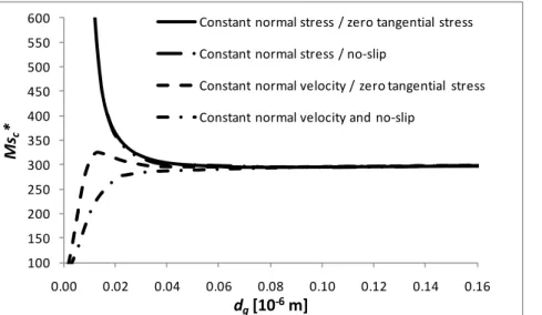
The no-slip and fixed normal velocity conditions are combined one by one with the conditions for the normal and tangential stresses, forming four different combinations for which the results are presented in Fig. 10. Otherwise, the stability analysis is performed as developed earlier in this paper. 100 150 200 250 300 350 400 450 500 550 600 0.00 0.02 0.04 0.06 0.08 0.10 0.12 0.14 0.16 Ms c * dg[10‐6m] Constant normal stress / zero tangential stress Constant normal stress / no‐slip Constant normal velocity / zero tangential stress Constant normal velocity and no‐slip
Fig. 10. The critical solutal Marangoni number as a function of the gas layer thickness for different kinds of hydrodynamic boundary conditions at the top boundary (10 wt% ethanol in water)
It turns out that the combination “constant normal stress / no-slip” shows no significant difference with respect to the originally used combination “constant normal stress / zero tangential stress”. This means that it is first of all the “constant normal stress” and the “constant normal velocity” conditions that make the difference for sufficiently small dg, the latter being
for smaller and smaller dg. To our knowledge, this peculiar instability is not discussed in the
literature, and we believe that it is caused by the evaporation-induced convective transport in the gas, acting similarly to a “wind” exerting some viscous stress back on the liquid layer. At large dg, with no restriction on the normal velocity at the top boundary, this “wind” is less
constrainted, and moves away without influencing significantly the instability in the liquid. However, at small dg and with a constant normal velocity at the top boundary, this “wind” gets
more restrained, hence increasing the viscous feedback on the liquid layer. For gas layer thicknesses larger than 30 nm, much more relevant in practice, it appears that the hydrodynamic boundary conditions have no significant influence on the stability analysis, which a posteriori justifies the choice made in (14).
6. Approximate model of the system
In the present section, we will build an approximate model of our system by keeping only the most important (from the viewpoint of the instability threshold) physical phenomena and show that the corresponding results are in a very good agreement with the complete analysis presented above. Such a validated approximate form of the model has an advantage that it involves easy-to-use analytical formulae. First, we will deduce an approximate reference solution. Then, we will show that the principal, solutal Marangoni mechanism of instability is well captured by the Pearson model with an appropriately defined Biot number, function of the wavenumber.
6.1 Approximate form of the reference solution
We have seen in section 3 that the Péclet numbers in the gas phase are quite small. It is easy to show that the temperature and concentration profiles for the reference solution are then linear in both the liquid and gas phases. In the liquid, these profiles are given by (29) and (31), whereas in
the gas we now have , , and , , , in lieu of (30) and
(32), where it has been taken into account that = 0 and . For simplicity, we also neglect the Soret effect here. Besides, the difference between the pressures , and is neglected in
Henry’s law.
A simple estimation shows that the smallness of the Péclet numbers is intimately related to the smallness of the vapor concentration (interestingly enough, this can be observed already from Table 3, where the two are very close indeed). We have ~ ~ ,
, while on the other hand ~ . Consequently, , ~ , indeed. Thus, consistent with using the linear profiles in the gas, we shall everywhere make simplifications corresponding to 1.
In particular, taking all this into account, the boundary conditions (19) and (23)-(25) become (for the reference profile)
, ,
, , , ,
, ,
all z = 1. T i an b c ,
at h s c e redu ed to a closed-form boundary condition for , :
, ,
, (63)
a , ,
t z = 1. For the linear profile (31), this yields the following equation for , , : , , , ,
, , ,
which is in fact a quadratic equation, having the fo , ,
llowing (physical) solution
, (64)
where
.
Having calculated ,
, , ,
, explicitely, some other quantities of interest are expressed as follows: , , , , (65) , , , 1 , (66) . (67)
We have thus been able to deduce an approximate analytical expression of the reference solution under the assumption of small vapor concentration in the gas phase (and the Soret effect has also been neglected both in the liquid and in the gas).
Table 5 provides some numerical values of important physical quantities for the approximate solution. The comparison of this table with Table 3 shows a very good agreement with the full approach.
Table 5. Characteristics of the reference state (approximate analysis) for different values of ( wt%10 ethanol in w , ater) , , , , , , 1.5 8.66*10-2 2.99*10-3 -1.65*10-1 -8.53*10-2 3.00*10-3 2 7.63*10-2 5.27*10-3 -1.52*10-1 -7.43*10-2 5.28*10-3 4 5.15*10-2 1.07*10-2 -1.06*10-1 -4.88*10-2 1.07*10-2 11 2.39*10-2 1.65*10-2 -4.97*10-2 -2.21*10-2 1.66*10-2 101 3.02*10-3 2.09*10-2 -6.31*10-3 -2.73*10-3 2.09*10-2
An important particular case corresponds to large gas-to-liquid thickness ratios ( 1), which is quite of interest given that the critical liquid thicknesses (for the onset of instability) has turned out to be rather small (section 5). Besides, it is in this case that the limit of small variations across the liquid layer ( , , ) is eventually attained and that the full formulation used in this paper proves to be most self-consistent. For instance, this is in the sense that the material properties of the liquid have all been fixed at (section 2), whereas at least some of them are rather sensitive to : these include the diffusion coefficient [24], the Soret coefficient (11)
and even – cf. Table 2. Also, , (neglected even in the full model by means of the quasi-stationary assumption) tends to zero as ∞ together with , , , whereas , (included in the full model) tends to a constant together with , , . For 1, the formulae (64)-(67) simplify just to
, , 1 , , , (68)
, , / , (69)
, , , , (70)
, , , , (71)
which compare well (less than 3% difference) with the full approach at H = 101. We find for , , , , and , , the values -6.50*10-3 K, -2.80*10-3 and 2.15*10-2 from (63)-(71), as compared to -6.30*10-3 K, -2.74*10-3 and 2.07*10-2 for the full model.
6.2 Stability analysis: Pearson-like model
The stability analysis based on the full model has shown that the solutal Marangoni effect is by far the most important instability mechanism. In the present section, we will thus neglect all the other effects when analyzing the stability. We will also continue assuming that convection in the gas can be neglected (neglecting , and in equation (46)). The term with in (46) can be neglected on the basis of 1 (assuming that the complex growth rate of the perturbation is
ith the diffusion time scale in the liquid). Thus, equation (46) becomes associated w
0 . Keeping in mind that
,
Cg = 0 at the top boundary, the solution is
. (72) The following boundary conditions can be deduced from (23)-(25) within the simplifications discussed in the previous subsection:
, 1
at z = 1, which have already been used when looking for the approximate solution for the ref rene ce profil Noe. w for the pertu a onrb ti s, they ecome b
, , , 1 , , at z = 1. Using (63) / 0, (73)
and (72), this can be reduced to the form
with a solutal “Bio n y
, t umber” given b , , 1 , , 1 2 coth 1 , , 1 , , 1 . (74) With (73), our formulation for the perturbation of the concentration field in the liquid layer is represented in Pearson’s terms [3]. Invoking besides the smallness of the evaporation Péclet
number in the liquid and neglecting the gas viscosity, we recover an equivalent form of Pearson’s formulation [3]. Thus, we can simply recur to his result for the marginal curve in order to describe our solutal Marangoni instability:
, 8 , . (75)
Here note that is the “true” solutal Marangoni number as is defined in (61). Fig. 11 represents (75) with (74) for a number of H values, where , , is taken according to (64).
(a) (b) 0 200 400 600 800 1000 1200 0 1 2 3 4 5 Full analysis Pearson‐like model Ms * k 0 200 400 600 800 1000 1200 0 1 2 3 4 5 Ms * k Full analysis Pearson‐like model (c) (d) 0 200 400 600 800 1000 1200 1400 0 1 2 3 4 5 Ms * k Full analysis Pearson‐like model 0 200 400 600 800 1000 1200 1400 0 1 2 3 4 5 Ms * k Full analysis Pearson‐like model
Fig. 11. The marginal curves in terms of the “true” solutal Marangoni number versus the wave number: comparison between the complete model of the present paper and the Pearson-like simplified model for H = 1.5 (a), H = 2 (b), H = 11 (c) H = 101 (d) (10 wt% ethanol in water) It shows an excellent agreement of the Pearson-like model with the full analysis. In particular, this suggests that convection in the gas phase is of minor importance indeed for different values of H. On the other hand, this underscores the importance of taking the Biot number as a function of the wavenumber of the perturbation as in (74) and not just the one defined by the uniform (reference) state, formally corresponding to 0 in (74), as it is sometimes the case in the literature [18]. Fig. 12(a) shows the critical liquid thickness as a function of the gas thickness for both models, while Fig. 12(b) presents the critical Marangoni number as a function of the gas thickness for both models as well, which also manifests an excellent agreement.