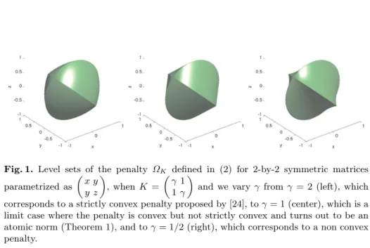
On learning matrices with orthogonal columns or disjoint supports

Hence, minimizing the total transmit power of the system under the user rate and antenna power limit constraints trans- lates into searching for the best “power transfer” scheme

This estimator is computed using a thresholding in an adapted orthogonal bandlet basis optimized for the noisy observed image.. In order to analyze the quadratic risk of this best

The decomposition on a ban- delet basis is computed using a wavelet filter bank followed by adaptive geometric orthogonal filters, that require O(N) operations.. The resulting

Such a principled method for addressing non-convexity consists in decomposing a non-convex objective function into the difference of convex functions, and then in solving the

Joint image reconstruction and PSF estimation is then performed within a Bayesian framework, using a variational algorithm to estimate the posterior distribution.. The image

This method, named MUS- CLE [1] for MUlti-channel Subspace-based Common poLe Estimation, has been applied to the biomedical signal analy- sis and is based on shift-invariance of

Ayant tir´ e un ´ echantillon d’une perle blanche et de trois perles noires d’une population de dix perles, quel est l’intervalle de confiance pour le nombre m de perles blanches

Finally, we derive in the general case partial generating functions, leading to another representation of the orthogonal polynomials, which also provides a complete generating