HAL Id: hal-00342599
https://hal.archives-ouvertes.fr/hal-00342599
Submitted on 27 Nov 2008
HAL is a multi-disciplinary open access
archive for the deposit and dissemination of
sci-entific research documents, whether they are
pub-lished or not. The documents may come from
teaching and research institutions in France or
abroad, or from public or private research centers.
L’archive ouverte pluridisciplinaire HAL, est
destinée au dépôt et à la diffusion de documents
scientifiques de niveau recherche, publiés ou non,
émanant des établissements d’enseignement et de
recherche français ou étrangers, des laboratoires
publics ou privés.
Does where you Gaze on an Image Affect your
Perception of Quality? Applying Visual Attention to
Image Quality Metric
Alexandre Ninassi, Olivier Le Meur, Patrick Le Callet, Dominique Barba
To cite this version:
Alexandre Ninassi, Olivier Le Meur, Patrick Le Callet, Dominique Barba. Does where you Gaze on an
Image Affect your Perception of Quality? Applying Visual Attention to Image Quality Metric. IEEE
International Conference on Image Processing, Sep 2007, San Antonio, United States. pp.169-172.
�hal-00342599�
DOES WHERE YOU GAZE ON AN IMAGE AFFECT YOUR PERCEPTION OF QUALITY?
APPLYING VISUAL ATTENTION TO IMAGE QUALITY METRIC
A. NINASSI
1,2, O. LE MEUR
11
THOMSON R&D France
1 Avenue Belle Fontaine
35511 Cesson-Sevigne, France
P. LE CALLET
2, D. BARBA
22
IRCCyN UMR 6597 CNRS
Ecole Polytechnique de l’Universite de Nantes
rue Christian Pauc, La Chantrerie
44306 Nantes, France
ABSTRACT
The aim of an objective image quality assessment is to find an automatic algorithm that evaluates the quality of pictures or video as a human observer would do. To reach this goal, researchers try to simulate the Human Visual System (HVS). Visual attention is a main feature of the HVS, but few studies have been done on using it in image quality assessment. In this work, we investigate the use of the visual attention information in their final pooling step. The rationale of this choice is that an artefact is likely more annoying in a salient region than in other areas. To shed light on this point, a quality assessment campaign has been conducted during which eye movements have been recorded. The results show that applying the visual attention to image quality assessment is not trivial, even with the ground truth.
Index Terms— Visual attention, image quality assessment, eye tracking, error pooling
1. INTRODUCTION
The best way to evaluate the quality of pictures or video is to ask hu-man observers to score it. The number of observers must be enough to obtain a representative Mean Opinion Score (MOS). Obviously, a quality assessment campaign cannot be used in imaging industry because it is time consuming, and it must be realized in normalized conditions. So, the challenge of image quality assessment is to de-sign automatic metrics which provide computed quality scores well correlated with those given by human observers.
Image quality metric may be classified into full reference met-rics (where both the original and impaired image are required), re-duced reference metrics (where a description of the original and the impaired image are both required), and no reference metrics (where only the impaired image is required). The most efficient metrics are based on the Human Visual System (HVS) [1, 2]. Visual attention is an important component of the HVS, which has been few stud-ied in relation with image quality assessment. However, one could intuitively expect that the use of visual attention information should improve the performances of a quality metric. For example, an arti-fact that appears on a region of interest is much more annoying than a degradation appearing on an inconspicuous area. So, a basic idea to improve a quality metric, through the use of the saliency infor-mation, is to give more importance to the degradation appearing on the saliency areas at the expense of the degradation appearing on the inconspicuous areas. Many full reference quality metrics are imple-mented in two stages. In the first stage, image distortion is localy
evaluated resulting in a distortion map. In the second stage, a spatial pooling function is used to combine the distortion map values into a single quality score.
In the literature, some authors try to use the visual attention information to improve the prediction capability of quality metrics [3, 4]. Nevertheless, the interpretation of these studies is compli-cated by the fact that two closely linked problems are not separately studied. The first problem is to compute the saliency information with visual attention models, and the second problem is to use the saliency information in the spatial pooling functions. The goal of this paper is to study the second problem lonely. Concerning this first point, a quality assessment campaign has been conducted dur-ing which eye movements have been recorded. Therefore, we know where observers have focused on exactly.
In this paper, different spatial pooling functions based on the saliency information are examined. We attempt to answer the fol-lowing question: does the use of saliency information in the pooling function improve the prediction accuracy of an image quality met-ric? As a quality assessment and eye tracking experiments have been conjointly conducted, real saliency information is available on one hand and the MOS on the other hand. This paper is decomposed as follows. Section 2 is devoted to the eye tracking experiments description. The different simple metrics based on saliency informa-tion are presented in secinforma-tion 3. Results are given and interpreted in section 4. Finally conclusions are drawn.
2. EYE TRACKING EXPERIMENTS 2.1. Eye tracking apparatus
In order to track and record real observers eye movements, exper-iments have been performed with a dual-Purkinje eye tracker from Cambridge Research Corporation(Fig. 1). The eyetracker is mounted on a rigid EyeLock headrest that incorporates an infrared camera, an infrared mirror and two infrared illumination sources. To obtain ac-curate data regarding the diameter of the subject’s pupil a calibration procedure is needed. The calibration requires the subject to view a number of screen targets at a known distance. Once the calibration procedure is completed and a stimulus has been displayed, the sys-tem is able to track a subject’s eye movement. The camera recorded a close-up image of the eye. Video was processed in real-time to extract the spatial location of the eye position. Both Purkinje reflec-tions are used to calculate the location. The guaranteed sampling frequency is 50 Hz and the accuracy is less than 0.5 degree.
Fig. 1. Eye tracking apparatus
2.2. Subjects
Twenty unpaid subjects participated to the experiments. All had nor-mal or corrected to nornor-mal vision. All were inexperienced observers (in video processing) and naive to the experiment. Before each trial, the subject’s head was positioned so that their chin rested on the chin-rest and their forehead rested against the head-strap. The height of the chin-rest and head-strap was adjusted so that the subject was comfortable and their eye level with the centre of the presentation display.
2.3. Quality assessment campaign
In this eye tracking experiment, participants have to assess picture quality as in every quality assessment campaigns. Experiments are conducted in normalized conditions (ITU-R BT 500-10). Images are displayed at a viewing distance of four times the height of the picture (80 cm), and their resolution is 512 × 512 pixels. The standardized method DSIS (Double Stimulus Impairment Scale) is used. Each observer views an unimpaired reference picture followed by an im-paired version of the same picture. Each picture is presented during 8s. Observer then rates the impaired video using an impairment scale containing five scores (imperceptible; perceptible but not annoying; slightly annoying; annoying; very annoying).
Ten unimpaired pictures are used in these experiments. The pic-tures were impaired by JPEG, JPEG2000 compression or through a blurring filter scheme. One hundred and twenty impaired pictures are then obtained.
2.4. Human saliency map
A saliency map topographically encodes for local conspicuity over the picture, and it is often compare to a landscape map [5] compris-ing peaks and valleys. A peak represents the observer’s regions of interest. To compute a saliency map, the eyetracker data are first parsed in order to separate the raw eye tracking data into fixation and saccade periods. The saliency map is computed in two different ways for each observer and for each picture.
The first way is based on the fixation number (FN) for each spa-tial location, so the saliency map SMF N(k)for an observer (k) is given
by: SMF N(k)(x, y) = NF P X j=1 ∆(x − xj, y − yj), (1)
where NF P is the number of fixation period detecting from the data
collected by the eyetracker, and ∆ is the Kronecker delta. Each fix-ation has the same weight.
The second way is based on the fixation duration (FD) for each spatial location. The saliency map SMF D(k)for an observer k is then
given by: SMF D(k)(x, y) = NF P X j=1 ∆(x − xj, y − yj) · d(xj, yj), (2)
where NF P and ∆ have the same meanings, and d is the fixation
duration.
To determine the most visually important regions, all the saliency maps are merged yielding to an average saliency map SM . The av-erage saliency map is given by:
SM (x, y) = 1 K K X k=1 SM(k)(x, y), (3)
where K is the number of observer.
Finally, the average saliency map is smoothed with a 2D Gaus-sian filter given a density saliency map DM :
DM (x, y) = SM (x, y) ∗ gσ(x, y) (4)
The standard deviation σ is determined in accordance with the accu-racy of the eye-tracking device. The average saliency map (example in Fig. 2) encodes the most attractive part of a picture when a large panel of observers is considered, so it reflects the average observer behavior.
3. SALIENCY-BASED SIMPLE QUALITY METRICS In the experiments, several simple saliency-based quality metrics are tested. These metrics adopted a two stage implementation. So for each metric, a distortion map is first evaluated from both the ref-erence and the impaired pictures. Then a single quality score is computed from the distortion map by using a saliency-based spatial pooling function.
3.1. Simple distortions maps
Two methods are used to compute the distortion maps. The first method is a simple absolute difference computed between the refer-ence and the impaired images. And the second method is the struc-tural similarity (SSIM) index [6] computed between the reference and the impaired images.
3.2. Saliency-based spatial pooling
The idea is to use the local saliency information to weight a local dis-tortion value. The general form of such spatial weighting approach is given by: Q = PW x=1 PH y=1wi(x, y) · q(x, y) PW x=1 PH y=1wi(x, y) , (5)
where Q is objective quality score, W and H are the width and the height of the picture respectively, wi(x, y) is the weight assigned to
the (x, y) spatial location (i defining the way to design the weight), and q(x, y) is the distortion value at the (x, y) spatial location.
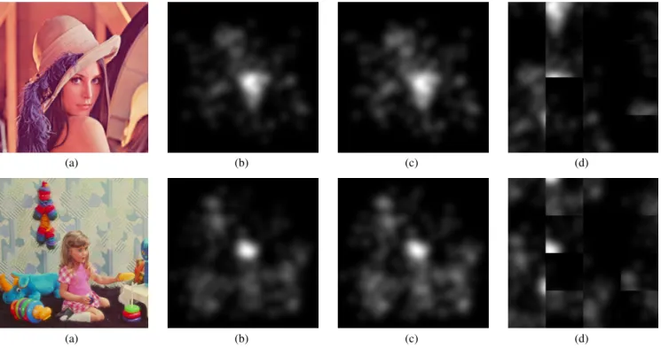
(a) (b) (c) (d)
(a) (b) (c) (d)
Fig. 2. (a) original images, (b) average saliency maps based on FD, (c) average saliency maps based on FN, and (d) switched versions of (b) defined in section 4
Four different functions wi, derived from the local saliency
in-formation, will be studied. These functions are given by: w1(x, y) = SMn(x, y) w2(x, y) = 1 + SMn(x, y) w3(x, y) = SM (x, y) w4(x, y) = 1 + SM (x, y) (6)
where SM (x, y) ∈ [0; Smax] is the unnormalized saliency map, and
SMn(x, y) ∈ [0; 1] is the normalized saliency map.
4. QUANTITATIVE ANALYSIS
The objective image quality measures are tested with two kinds of distortion map (cf. subsection 3.1), with the four different spatial pooling function (cf. subsection 3.2), and with two different kinds of saliency map (cf. subsection 2.4). A switched version of the saliency maps is also tested (cf. Fig. 2c). In this switched version, the saliency map is split into 16 blocks and each block is replaced with another one. Therefore, the saliency information is lost but the cover ratio and the dynamic range remain the same. The picture database de-scribed in subsection 2.3 is used.
Prior to evaluate the objective image quality measures, a psy-chometric function is used to transform the objective quality score Q (cf. Eq. 5) in predicted MOS (MOSp), as recommended by the Video Quality Expert Group [7](VQEG). The psychometric function is given by:
M OSp = b1
1 + e−b2∗(Q−b3), (7)
where b1, b2 and b3 are the three parameters of the psychometric function.
To evaluate the impact of the saliency information, the differ-ent saliency-based quality metrics are compared to convdiffer-entional ap-proaches (wi= 1 in Eq. 5).
4.1. Mean Observer Behavior
In this subsection, the mean observer behavior is studied, so the av-erage saliency maps are used here. The objective quality metrics are evaluated by comparing the MOS and the MOSp on the whole database using the linear Correlation Coefficient (CC) and the Root Mean Square Error (RMSE). The results are shown in table 1 and table 2.
For the distortion maps based on absolute difference (cf. ta-ble 1), a prediction improvement is observed with the w3 weight
function regardless of the saliency used (FN or FD). CC are 0.83 Pooling FD (saliency) FN (saliency) Saliency wi CC RMSE CC RMSE
None 1 0.742 0.814 0.742 0.814 w1 0.510 1.044 0.504 1.049 Real w2 0.733 0.826 0.731 0.829 w3 0.830 0.678 0.821 0.692 w4 0.825 0.686 0.754 0.797 w1 0.387 1.142 0.388 1.140 Switched w2 0.725 0.836 0.722 0.840 w3 0.764 0.815 0.750 0.835 w4 0.778 0.787 0.744 0.813
Table 1. Performance Comparison of objective quality metrics. The Absolute difference is used to generate the distortion map.
Num-ber) saliency maps respectively, against 0.74 without the use of the saliency information. A prediction improvement is also observed with the w4weight function but only with the FN saliency. CC is
0.825 with the FD saliency, against 0.74 without the saliency infor-mation. No other prediction improvement is observed, but some pre-diction worsenings are observed. For example, with w1weight
func-tion, the CC are 0.51 and 0.5 for the FD and the FN saliency maps re-spectively, against 0.74 without the saliency information. The same observations are done with the RMSE.
With the switched maps, no meaningful prediction improvement is observed in terms of CC and RMSE, and even sometimes some prediction worsenings. The same observation is done with the w3
and w4weight functions, so it means that the prediction
improve-ment observed with the real saliency map and this two weight func-tions are not due to chance.
For the SSIM distortion maps (cf. table 2), no meaningful pre-diction improvement is observed in terms of CC and RMSE regard-less of the weight functions and the kind of saliency used.
Pooling FD (saliency) FN (saliency) Saliency wi CC RMSE CC RMSE
None 1 0.827 0.686 0.827 0.686 w1 0.820 0.696 0.821 0.695 Real w2 0.827 0.686 0.827 0.686 w3 0.820 0.696 0.821 0.695 w4 0.825 0.688 0.828 0.685 w1 0.811 0.713 0.818 0.701 Switched w2 0.827 0.684 0.828 0.684 w3 0.811 0.713 0.818 0.701 w4 0.826 0.685 0.828 0.684
Table 2. Performance Comparison of objective quality metrics. The SSIM index is used to generate the distortion map.
Consequently, the positive impact of the saliency information on the prediction is not as clear as expected, and the prediction is not really improved, even if there are exceptions with w3in the context
of using the absolute difference distortion maps. The four weight functions used favour the distortion appearing on the saliency area to the detriment of the other area. The w1and w3weight functions
are more penalizing for the distortion appearing in the inconspicuous areas, than the w2 and w4 weight functions. The weight functions
and the average saliency map building can be suspected to explain the non-improvement of the prediction. The latter is examined in the next subsection.
4.2. Particular Observer Behavior
Rather than to take heed of the average observer, the behavior of 8 particular observers are studied, their saliency maps and their qual-ity notes are used to evaluate the objective qualqual-ity metrics. For each observer studied, the objective quality metrics is evaluated by com-paring the quality notes and the predicted quality notes on the whole database, using the linear Correlation Coefficient (CC) and the Root Mean Square Error (RMSE).
For the distortion maps based on absolute difference, no mean-ingful prediction improvement is observed regardless of the weight functions, the kind of saliency used, and the observer. The mean of the CC variations are -0.08 and -0.07 for the FN and the FD saliency maps respectively. The results are quite variable from one observer to another.
For the SSIM distortion maps, the observations are the same. There are no meaningful prediction improvement regardless of the weight functions, the kind of saliency used, and the observer. The mean of the CC variations are -0.01 and -0.02 for the FN and the FD saliency maps respectively. The results are quite variable from one observer to another.
Consequently, the average saliency map construction does not explain the non-improvement of the prediction when the mean ob-server behavior is considered. A meaningful prediction improve-ment is not observed, even if, for one observer, the real saliency in-formation corresponding to where he gazes to give his quality score is used.
5. CONCLUSION
Four attention-based spatial pooling functions have been tested in the context of image quality assessment. The visual attention recorded during a quality assessment campaign is used. The results show that the prediction improvement is not clearly established. The prediction improvements on some particular cases show that the visual atten-tion informaatten-tion can be interesting, but the general non-improvement suggests that the way to take in account the visual attention cannot be limited to a simple spatial pooling. These results are not con-sistent with those of previous work [3, 4], where the prediction im-provements could be explained by the improvement of the spatial coherence of the errors rather than by the saliency information itself. New studies are required to well understand the visual atten-tion mechanisms in an image quality assessment context. During his evaluation process, an observer can spend less time on an obvious degradation than on a less important degradation. In the former, the saliency is low but the contribution to the quality score is high, and in the latter the saliency is high and the contribution to the quality score is lower. It seems that the saliency information and the degradation intensity have to be jointly considered.
6. REFERENCES
[1] S. Daly, “A visual model for optimizing the design of image processing algorithms”, IEEE ICIP, pp. 16–20, 1994.
[2] P. Le Callet and D. Barba, “Perceptual color image quality met-ric using adequate error pooling for coding scheme evaluation”, SPIE HVEI, 2002.
[3] W. Osberger, N. Bergmann, and A. Maeder, “An automatic im-age quality assessment technique incorporating higher level per-ceptual factors”, IEEE ICIP, pp. 414–418, 1998.
[4] R. Barland and A. Saadane, “Blind quality metric using a per-ceptual importance map for JPEG-2000 compressed images”, IEEE ICIP, pp. 2941–2944, 2006.
[5] D. S. Wooding, “Eye movements of large population : II. de-riving regions of interest, coverage, and similarity using fixation maps”, Behavior Research Methods, Instruments and Comput-ers, vol. 34(4), pp. 509–517, 2002.
[6] Z. Wang, A. C. Bovik, H. R. Sheikh, and E. P. Simoncelli, “Im-age quality assessment: From error visibility to structural simi-larity”, IEEE Trans. on Image Processing, vol. 13, pp. 600–612, 2004.
[7] VQEG, “Final report from the video quality experts group on the validation of objective models of video quality assessment”, March 2000, http://www.vqeg.org/.