Diagnosing performance variations by comparing multi-level execution traces

Titre:

Title

:

Diagnosing performance variations by comparing multi-level

execution traces

Auteurs:

Authors

: François Doray et Michel R. Dagenais

Date: 2016

Type:

Article de revue / Journal article

Référence:

Citation

:

Doray, F. & Dagenais, M. R. (2016). Diagnosing performance variations by comparing multi-level execution traces. IEEE Transactions on Parallel and

Distributed Systems, 28(2), p. 462-474. doi:10.1109/tpds.2016.2567390

Document en libre accès dans PolyPublie

Open Access document in PolyPublie

URL de PolyPublie:

PolyPublie URL: https://publications.polymtl.ca/2961/

Version: Version finale avant publication / Accepted version_{Révisé par les pairs / Refereed} Conditions d’utilisation:

Terms of Use: Tous droits réservés / All rights reserved

Document publié chez l’éditeur officiel

Document issued by the official publisher Titre de la revue:

Journal Title: IEEE Transactions on Parallel and Distributed Systems (vol. 28, no 2) Maison d’édition:

Publisher: IEEE URL officiel:

Official URL: https://doi.org/10.1109/tpds.2016.2567390 Mention légale:

Legal notice:

© 2016 IEEE. Personal use of this material is permitted. Permission from IEEE must be obtained for all other uses, in any current or future media, including

reprinting/republishing this material for advertising or promotional purposes, creating new collective works, for resale or redistribution to servers or lists, or reuse of any copyrighted component of this work in other works.

Ce fichier a été téléchargé à partir de PolyPublie, le dépôt institutionnel de Polytechnique Montréal

This file has been downloaded from PolyPublie, the institutional repository of Polytechnique Montréal

Diagnosing Performance Variations by

Comparing Multi-Level Execution Traces

François Doray Student Member, IEEE and Michel Dagenais, Senior Member, IEEE

F

Abstract—Tracing allows the analysis of task interactions with each

other and with the operating system. Locating performance problems in a trace is not trivial because of their large size. Furthermore, deep knowledge of all components of the observed system is required to decide whether observed behavior is normal.

We introduce TraceCompare, a framework that automatically iden-tifies differences between groups of executions of the same task at the userspace and kernel levels. Many performance problems manifest themselves as variations that are easily identified by our framework. Our comparison algorithm takes into account all threads that affect the completion time of analyzed executions. Differences are correlated with application code to facilitate the correction of identified problems. Performance characteristics of task executions are represented by a new data structure called enhanced calling context tree (ECCT).

We demonstrate the efficiency of our approach by presenting four case studies in which TraceCompare was used to uncover serious per-formance problems in enterprise and open source applications, without any prior knowledge of their codebase. We also show that the overhead of our tracing solution is between 0.2% and 9% depending on the type of application.

Index Terms—Performance analysis, Tracing, Software visualization,

Concurrency, Operating systems.

1

I

NTRODUCTION

P

ERFORMANCEis a critical requirement for many appli-cations. Long delays are among the main sources of user frustration [1] and have a significant impact on revenue [2]. Despite that, it is often difficult for a single developer to understand all the factors that influence the performance of an application. This is mainly due to the multiple levels of abstraction that are supposed to ease software development: frameworks, operating systems and virtualization. Further-more, diagnosing performance problems is hard because they don’t necessarily trigger error conditions and often can’t be easily reproduced.

Tracing is a technique that consists of recording events during the execution of a system. Events have a timestamp, a type and a payload. Tracing is well suited to analyze performance problems. Popular tracers achieve low over-head, which allows them to be enabled on production systems to capture bugs that occur infrequently. Tracing F. Doray ([email protected]) and M. Dagenais ([email protected]) are with the Computer and Software Engineering Department, Ecole Polytechnique de Montreal.

Manuscript received May X, 2015; revised Month Y, 2015.

provides detailed chronological information, unlike profil-ing that only provides global statistics for a given time range. A trace can, for example, reveal what happened on the whole system during a long system call issued by a process of interest. However, unless userspace applications are carefully instrumented, it is hard to relate the low-level events of a trace to the higher-level logic. Also, it is hard to locate abnormal behavior in the overwhelming amount of information contained in a trace, without deep knowledge of the observed system.

Our objective was to build a tool that automatically highlights differences between two sets of executions of the same task. The comparison must take into account all factors that have an impact on performance, including off-CPU wait time and interferences between processes. Also, it must relate any difference found with the relevant source code, a requirement that is crucial to ease the diagnosis and correction of problems [3]. Our tool should allow a developer that doesn’t have a full knowledge of a system to discover and fix performance variations caused by fac-tors such as configuration changes, programming errors or sporadic competition between tasks.

This paper introduces TraceCompare, a trace comparison tool and underlying algorithms that achieve all these goals. After reviewing relevant existing work, we describe a data model to summarize performance characteristics of task executions. We then explain how to record detailed multi-level events during an execution and how to process them to generate a database of executions based on our data model. We introduce a GUI that facilitates the identification of dif-ferences between groups of executions. We describe four real performance problems found in enterprise and open-source applications and explain how they were diagnosed using TraceCompare. Finally, we measure the overhead incurred by each component of our solution and show that it is low enough for use on production systems.

2

R

ELATED

W

ORK

2.1 Analyzing Execution Traces

Our group proposed using a state history to simplify and accelerate the analysis of large traces [4]. A state history is built incrementally while a trace is read. It keeps track of various attributes such as the current running thread on each CPU or the total number of bytes read from the disk since the beginning of the trace. An efficient data structure

has been designed to allow fast queries about the value of an attribute at a given time within a state history that exceeds the size of the main memory. TraceCompass1_relies on this data structure for its interactive views. State histories allow the computation of system metrics for any given time interval in logarithmic time [5].

2.2 Extracting Task Executions from a Trace

Our group developed a critical path algorithm to efficiently retrieve all execution segments that contribute to the latency of a task [6]. It uses the sched_wakeup event of the Linux kernel to identify dependencies between multiple threads on the same host, and TCP packets matching to identify dependencies between threads that span multiple hosts. The analysis works well with any kind of application because it requires no userspace instrumentation. While this tool indi-cates in which threads time is spent, it does not relate this information to userspace functions, which makes it difficult to use for fixing application code. Also, the interactive view shows only one execution at a time, which is impractical to compare latency among a great number of executions. Perfscope provides a heuristic to find userspace functions associated with events from a kernel trace [7]. However, the results are not always accurate.

A portion of the requests received by Google are traced by Dapper [8]. The tool reconstructs the flow of individual requests using events generated by the company’s commu-nication libraries. Developers can access summary statistics or inspect individual requests through a Web interface. Filters help them find executions that contain abnormal latencies. Dapper relies on the fact that all communications go through a Google’s library and isn’t designed for hetero-geneous environments.

2.3 Comparing Task Executions

The "Frames" mode of Chrome developer tools presents the processing time of frames using bar charts [9]. Slow frames are shown as tall bars. Colors within each bar indicate in which states time was spent (JavaScript, rendering, GC...). Developers can determine why a frame took more time than others by comparing the distribution of time per state between different frames. The scope of this tool is limited to the browser. It doesn’t take into account interactions be-tween processes. A similar view was developed to compare the states in which real-time tasks spend their time from a kernel point of view [10].

A differential flame graph is a visualization tool to com-pare two CPU profiles [11]. It shows stack frames as super-posed rectangles. The width of a rectangle is proportional to the time spent in a stack frame within the second profile. The color shows the difference between the time spent in a stack frame in the two profiles. Because a profile only provides total counts for a given period, this tool cannot reveal the cause of infrequent latencies. Flame graphs have been adapted to show different metrics, but they have never presented all the work done on the critical path of a task.

Comparisons of CPU profiles have been used to diag-nose performance variations between multiple versions of

1. http://projects.eclipse.org/projects/tools.tracecompass

the same application [12], evaluate the impact of configura-tion changes [13] and assess the scalability on an applicaconfigura-tion with respect to the size of its input [14].

TraceDiff is a visualization tool to compare two function call traces [15]. A function call trace contains an event for every function entry and exit. TraceDiff displays two such traces simultaneously as mirrored icicle plots. Correspond-ing function calls are connected by hierarchical edge bun-dles. This facilitates the identification of individual function calls that didn’t take the same time or weren’t executed in the same order in the two traces. However, it doesn’t al-low simultaneous comparison of many executions to reveal trends. Also, generating function call traces is costly. Other researchers have developed a heuristic to get an approxi-mate function call trace with low overhead [16]. Efficient algorithms to compute the optimal alignment between two function call traces have also been developed [17].

Comparison of system call traces recorded on different operating systems has been used to detect intrusions [18]. Since some variations are inherent to the use of different op-erating systems, the authors transform low-level events into higher-level concepts to allow a meaningful comparison. Their algorithm computes a correlation score for two traces, but doesn’t show individual differences. Also, it doesn’t take timing into account.

2.4 Statistical CPU Profiling

A statistical CPU profiler is a tool that can record the full call stack of a program at regular intervals. This reveals which functions use more CPU time, with minimal overhead. While statistical profilers don’t provide the chronological order of events, which is required to analyze interactions between multiple tasks, some of these techniques could be reused to get insight into the logic of userspace programs, without requiring manual instrumentation.

The CPU profiler of Google Perftools is a dynamic li-brary, to link with programs to analyze [19]. In its initializa-tion phase, it registers a SIGPROF signal handler and starts an ITIMER_PROF timer. The timer is decremented when-ever a thread of the process consumes CPU time. When a thread reaches the expiration of the timer, the SIGPROF signal handler is invoked and captures the thread’s call stack. Alternatively, perf leverages support from the Linux operating system to profile program [20].

Capturing the call stack of a program, when compiled with the frame pointer, is just a matter of following a linked list formed by base pointers pushed on the stack. However, in order to keep the ebp register available for computation, GCC does not preserve the frame pointer for x86-64 binaries, since version 4.6.02_{. The .eh_frame sections of these} Executable and Linkable Format (ELF) binaries provide rules to restore the register values of the previous (oldest) stack frame from any instruction [21]. A call stack can be captured by applying these rules to retrieve the value of the instruction pointer at each stack frame. The .eh_frame section is present, even when debugging information is stripped, because it is required to handle exceptions.

2. https://gcc.gnu.org/onlinedocs/gcc-4.6.0/gcc/ Optimize-Options.html

The libuwind library implements the logic to capture call stacks using rules from the .eh_frame section. For good performance, it recognizes stack frames that use a standard layout, and caches that information to handle them with an optimized algorithm when they are encountered again [22]. Google Perftools relies on libunwind to cap-ture call stacks online. Instead, perf records two pages of memory and runs libunwind offline [23]. This reduces the computation overhead, but leads to huge profile files.

A CPU profile can be represented using a calling context tree (CCT); a data structure introduced by [24] and reused by [3], [25]. In a CCT, each node represents a call stack. The children of a node associated with a call stack C of size n are associated with call stacks of size n + 1 prefixed with C. The root of the CCT represents the empty call stack. Each node is annotated with the time spent in its associated call stack. Unlike a call tree which contains a distinct node for each individual function call, a CCT combines all calls associated with the same call stack into a single node. A CCT does not show interactions between different threads.

3

S

OLUTION

In this section, we present the design and implementation of TraceCompare. First, we describe a data model to store performance characteristics of task executions in a database. Second, we explain how to efficiently record the information required to build this database through tracing. Third, we explain algorithms used to build the database from traces. Finally, we present the user interface that highlights dif-ferences between groups of task executions. The general architecture of the tool is summarized in Fig. 1.

Database Trace Trace Comparison View Builder

Fig. 1. Architecture of TraceCompare

3.1 Data Model

We introduce a new data structure called enhanced calling context tree (ECCT) to represent the performance character-istics of task executions. An ECCT can describe any kind of latency that occurs during a task execution as well as the detailed context of each latency. Our database of executions and the algorithms that power our GUI rely on this data structure.

For executions that spend all their time on the CPU and involve a single thread, the structure of the ECCT is identical to that of a CCT. We annotate each node with the time spent in the associated call stack during the analyzed execution. Optionally, more annotations such as the number of page faults or amount of memory allocated in the call stack can be added.

For executions that contain off-CPU wait times or that involve multiple threads (possibly distributed on multiple hosts), the CCT is enhanced so that all factors that contribute

to the total time of an execution are taken into account. First, for any off-CPU wait time, an artificial function named after the wait reason (timer, block device, network, preemp-tion...) is pushed on the stack. Second, whenever a thread is waiting for another thread, the stack of the second thread is concatenated to that of the first thread. This rule can be applied recursively as many time as required when there is a chain of dependencies between threads. The dependencies can be either direct (a thread is waiting for another thread to compute a result or perform an action) or indirect (a thread is waiting for another thread to release a resource such a the CPU or a mutex).

One might be concerned about the case where indirect dependencies between two different task executions lead to the concatenation of their ECCT. A safeguard could be added to stop the recursion in such a case. However, in our experience, it was rather useful to be able to see which parts of an execution could block other executions. Programs that use a limited number of worker threads have ECCTs of reasonable size, even when a lot of requests are queued.

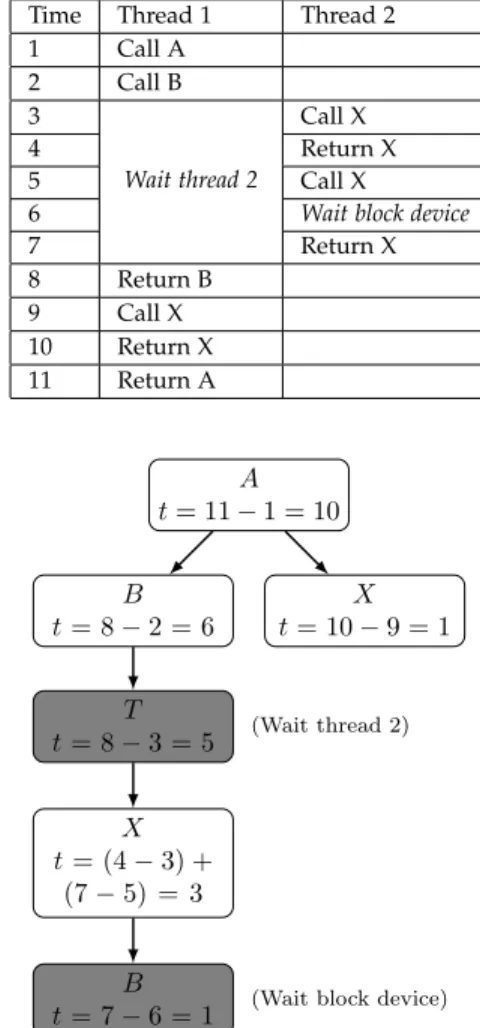
Fig. 2 shows the expected ECCT for a sample sequence of events.

Time Thread 1 Thread 2 1 Call A 2 Call B 3 Wait thread 2 Call X 4 Return X 5 Call X

6 Wait block device

7 Return X 8 Return B 9 Call X 10 Return X 11 Return A A t = 11− 1 = 10 B t = 8− 2 = 6 T t = 8− 3 = 5 X t = (4− 3) + (7− 5) = 3 B t = 7− 6 = 1 X t = 10− 9 = 1 (Wait thread 2)

(Wait block device)

Fig. 2. ECCT for a Sample Sequence of Events

3.2 Tracing Task Executions

We now describe the techniques used to gather the informa-tion required to build the data model that we just described.

The Linux Trace Toolkit Next Generation (LTTng)3_tracer can record events from the Linux kernel and from userspace applications into a single trace [26]. It is also designed to have a minimal overhead on traced systems. It is therefore well suited to our goal of collecting all the factors that contribute to the execution time of tasks in production environment.

3.2.1 Execution Delimiters Events

A single trace usually contains events belonging to multiple executions that occured in series or in parallel. To allow a comparison between different executions, it is necessary to demultiplex these events. To do so, the trace must provide a way to identify the start and end points of each execution. Sometimes, existing events of the Linux kernel can be used for this purpose. For example, the syscall_exit_accept event (generated when a connection is accepted on a socket) and the syscall_entry_shutdown event (gen-erated when a connection is closed) correctly delimit re-quests received by an Apache server. An advantage of using existing events is that no access to the source code is required. When no existing events can act as delimiters, LTTng-UST probes must be inserted statically in the source code. Different probe types can be used to delimit different execution types. That way, our analysis tool is able to tag executions when they are inserted in the database so that the GUI only allows comparison of executions of the same type.

3.2.2 Critical Path Events

When an execution involves a single thread running 100% of the time on a CPU, it is trivial to retrieve its events from the trace: we simply look for events between the start and end points on the execution’s thread. However, in parallel systems, most executions require collaboration between multiple threads. TraceCompare relies on the crit-ical path algorithm proposed by our group and introduced in section 2.2 to find all thread segments that contribute to the total time of an execution. This algorithm requires a few events of the Linux kernel to work properly.

The sched_switch event indicates that a new thread starts running on a CPU. Its payload gives the tid of the new thread and tells whether the previous thread was preempted or blocked. The sched_wakeup events is emitted when a blocked thread becomes ready to run. The reason why the thread was blocked can be deduced from the context in which the sched_wakeup event is emitted. For example, if the event is emitted from a block device related interrupt, it means that the waked up thread was waiting for a block device request. The irq_handler_entry, irq_handler_exit,

hrtimer_expire_entry, hrtimer_expire_exit,

softirq_entry and softirq_exit events allow

to keep track of interrupts handled on each CPU in order to correctly interpret sched_wakeup events. The

inet_sock_local_in and inet_sock_local_out

events provide the sequence number and flags of TCP packets. Using these fields, incoming and outgoing packets can be matched to uncover dependencies between threads that communicate through TCP.

3. https://lttng.org

3.2.3 Call Stacks Events

TraceCompare must make it easy to relate performance variations, between multiple executions of the same task, to erroneous logic in userspace applications. LTTng allows developers to insert custom tracepoints in their code to correlate kernel events with the logic of userspace appli-cations. This is, however, not suited to the requirements of TraceCompare. Indeed, we want to build a solution that developers can use on systems that they don’t fully under-stand. Requiring to create tracepoints would represent a ma-jor maintenance burden and developers would inevitably forget to instrument important parts of their applications. Requiring instrumentation of third-party libraries would be even harder.

TraceCompare gets insight into userspace applications without any manual instrumentation by capturing their call stack in two different contexts. The first context in which the stack is captured is at the expiration of a timer that is decremented when a thread is running, a technique already used by statistical profilers. However, that doesn’t provide information about call stacks that block the thread. An interesting observation is that most blockings occur within system calls. For example, a thread can block while it waits for a mutex to be available (futex()) or for data to be read from a file (read()). Therefore, also capturing the call stack on system calls gives a complete portrait of the contexts in which a thread spends its time.

Statistical CPU profilers can keep track of the number of captured samples per call stack using an hash table. This is sufficient to generate summary statistics for the full ana-lyzed period. However, our goal is to provide per-execution statistics and we don’t know beforehand to which execution a thread segment belongs to. Furthermore, during our of-fline analysis, we need to be able to correlate kernel events to userspace stacks and to combine multiple userspace stacks occuring simultaneously on different threads. For that reason, a timestamped LTTng-UST event is emitted every time a stack is captured. Stacks captured while userspace code is running produce a cpu_stack event while stacks captured during system calls produce a syscall_stack event.

To get the stacks of a process captured, the lttng-profiledynamic library must be preloaded into it. The library uses the same technique as Google Perftools to generate a SIGPROF signal at regular intervals, from which cpu_stackevents are generated.

The SIGPROF signal must also be sent to capture the userspace stacks associated with system calls. Unfortu-nately, experimentations show that handling a signal can take longer than the duration of some fast system calls. Therefore, sending a signal and capturing the stack for each system call can add a prohibitive overhead to programs making a lot of short system calls. The problem is that, unlike statistical CPU profiling, which generates a fixed number of events per time unit and per thread, the over-head of this instrumentation is proportional to the number of system calls. To solve that, we decided to capture the userspace stack only for system calls with a duration above a threshold. This effectively sets a reasonable upper limit on the rate of events generated by each thread. Because performance is generally not affected by very short system

calls, this doesn’t undermine the accuracy of our analysis. We found that a 100 µs threshold was a good compromise between precision of the analysis and low overhead.

The duration of system calls is tracked by a kernel module. When it is loaded, the lttng-profile library registers the process with the kernel module through an ioctlinterface. The kernel module uses the TRACE_EVENT mecanism [27] to register callbacks that are executed at the entry and exit of system calls. On system call entry, the kernel module checks whether the issuing process is registered. If so, the current timestamp is saved in a read-copy update (RCU) hash table with the source thread id as the key. On system call exit, the duration of the system call is computed, if the start time is available in the hash table. If the duration is higher than a threshold, a SIGPROF signal is sent to the source thread. lttng-profile catches the signal and captures the call stack, as soon as the control goes back to userspace.

The first time that a thread does a system call, an entry is added to the hash table and it is reused until the thread exits. Therefore, most of the time, tracking the duration of a system call simply requires one update and one lookup in the hash table, two very efficient operations.

Our SIGPROF signal handler uses libunwind to cap-ture call stacks. This library is the state of the art to capcap-ture call stacks when the frame pointer is absent. We contributed two important optimizations to libunwind in order to accelerate the backtrace operation even more. First, we removed system calls that blocked signals while shared data structures were accessed. This was necessary to guarantee the reentrancy of libunwind. However, since we always invoke the library within SIGPROF signal handlers, and since Linux doesn’t allow nested signals of the same type, it is valid to remove that protection in our case. Second, we replaced a loop that restored the value of all registers by more efficient code that restores only the registers that are really needed.

The call stack events generated by our library contain sequences of addresses, instead or human-readable function prototypes. This reduces the tracing overhead and the size of the trace. However, for analysis purposes, full symbols are required. Therefore, we record events that provide the base address of dynamic libraries. Those allow us to transform captured addresses into library offsets. Then, we parse ELF binaries offline, to retrieve function prototypes.

3.3 Building a Task Executions Database

We described how the data required by our analysis can be collected through tracing. We now explain how to process this data to build a database of task executions. The ECCT data structure introduced in section 3.1 is used to represent the performance characteristics of each task execution in the database.

The TraceCompare builder reads the events of a trace in chronological order. When it encounters an event associated with the beginning of an execution, the current timestamp and current thread are saved in a list of pending executions. Then, when the event marking the end of the execution is encountered, the following steps are performed:

1) Compute the critical path of the execution.

2) Generate an ECCT for the execution. 3) Compute global execution metrics.

4) Insert the execution’s ECCT and metrics in a database.

3.3.1 Critical Path

TraceCompare computes the critical path of an execu-tion using the algorithm proposed by our group. The inputs of the algorithm are start and end points, both (thread id, timestamp) pairs, and a graph of dependencies between threads. The output is a list of segments belonging to the critical path of the execution, each characterized by a thread id, a thread status, a start timestamp and an end timestamp. The thread status takes one of the following val-ues: running, preempted, interrupted, waiting for another thread or waiting for the operating system (block device, network, timer or user input).

The graph of dependencies between threads is built incrementally while the trace is read. Only nodes generated by events that occured during an execution are required to compute its critical path. Therefore, the critical path of an execution can be computed as soon as its end event is encountered (before the full trace has been read).

3.3.2 ECCT

The next step of the analysis is to generate the ECCT of the execution from the stacks that appear on each segment of its critical path. Backtracking to reread events of the trace, every time the end of an execution is encountered, would be highly inefficient. Instead of that, we generate a state history while we read the trace. Efficient State History Trees were proposed by our group and described in section 2.2. Using them for comparison of executions is an original contribution. When the time comes to generate the ECCT of an execution, the required information is obtained by querying the state history. The evolution of the following attributes is tracked in our state history:

• threads/[tid]/cpu: The CPU on which the thread tid is running.

• threads/[tid]/stack: The call stack of the thread tid.

• cpus/[cpuid]/thread: The thread running on the CPU cpuid.

• blockdevice/threads: Threads waiting for a block device.

The algorithm presented in Fig. 3 generates the ECCT of an execution from its critical path and a state history. 3.3.3 Execution Metrics

It is convenient to be able to filter executions based on a wide range of metrics when performing a comparison. For example, we might want to compare executions that generated a lot of page faults against those that generated a few, or executions that allocated a lot of memory against those that allocated a few.

Depending on the events that are present in the source trace, we can keep track of the evolution of different metrics in the state history. Then, when we process an execution, we compute metrics for each segment of its critical path.

Input: critical pathC, state historyH, stack of threadsT, ECCTE . TandEare empty in the first recursive call to this function. 1: for alle ∈ Cdo

2: UPDATETHREADSTACK(H,T,e.tid,e.start) 3: ife.status=running then

4: stacks ←QueryHfor stacks of threadtidin time range[e.start, e.end].

5: for alls ∈ stacksdo

6: if T.SIZE> 2 then

7: s.val ←CONCATENATE(T[−2].stack, thread,s.val) 8: end if

9: E.INSERT(s.val,s.duration) 10: end for

11: else ife.status=preempted then

12: cpuId ←QueryHfor CPU of threadtidat timee.start. 13: threads ←QueryHfor threads running on CPUcpuIdin

time range[e.start, e.end]. 14: for allt ∈ threadsdo

15: epreempt←(t.val, running,t.start,t.end)

16: GENERATEECCT({epreempt},H,T,E)

17: end for

18: else ife.status=blockdevice then

19: threads ←QueryHfor threads using a block device in time range[e.start, e.end].

20: for allt ∈ threadsdo

21: s ←QueryHfor stack of threadt.valat timet.start. 22: s ←CONCATENATE(T[−1].stack, block device,s) 23: E.INSERT(s,e.duration/threads.size)

24: end for

25: else

26: s ←CONCATENATE(T[−1].stack,e.status) 27: E.INSERT(s,e.duration)

28: end if

29: UPDATETHREADSTACK(H,T,e.tid,e.end) 30: end for

Fig. 3. Function GENERATEECCT Generates the ECCT of an execution.

Input: state historyH, stack of threadsT,tid,ts 1: fori ←0to T.SIZE− 1do

2: ifT[i].tid = tidthen

3: T.RESIZE(i) 4: end if

5: end for

6: s ←QueryHfor stack of threadtidat timets. 7: if T.SIZE>0then

8: s.val ←CONCATENATE(threads[−1].stack, thread,s.val) 9: end if

10: T.PUSH((tid, s.val))

Fig. 4. Function UPDATETHREADSTACK: Puts the enhanced stack of a thread at the top of a stack of threads.

The values of each segment are then combined into a global metric, on which filters can be applied in our comparison view.

3.3.4 Database

Once the ECCT and the global metrics of an execution have been computed, they are added to the executions database. An interesting observation is that there is no need to dupli-cate the structure of the ECCT for each execution. A generic ECCT can be formed by the union of all the other ECCTs. Its structure along with the function prototype of each node are stored once in the database. Each execution record can then refer to the nodes of the generic ECCT to specify metrics. Because the ECCTs issued from different executions of the same task normally have a similar structure, this original technique greatly reduces the size of the database.

3.3.5 Garbage collection

Two data structures are built incrementally while the trace is read: a graph of dependencies between threads and a state history tree. The size of both these data structures is proportional to the number of events read. For huge traces, storage of all this data might be a concern. Fortunately, the nodes added to the graph of dependencies, before the first event of an execution is read, are not needed to compute its critical path. Similarly, the intervals of the state history tree, that end before the begininnig of an execution, are not needed to compute its ECCT or global metrics. Therefore, whenever the available memory is getting low, it is possible to discard the parts of the data structures that won’t be needed to process the pending executions. In addition to reducing memory usage, this strategy improves the time complexity of queries in both data structures. They become logarithmic with respect to the average size of an execution, instead of logarithmic with respect to the size of the ana-lyzed trace.

3.4 Comparing Task Executions

The database of executions is used to populate a web-based view that allows interactive comparisons between groups of executions. The view is divided in three parts: the filters, the flame graph and the list of executions. An obvious benefit of providing a web-based view is that it facilitates collaboration. Anybody can easily share a link to its findings in a bug report, to help others fix the problem quickly. This is much more convenient than sharing huge trace files, let alone asking others to reproduce a complex bug themselves. 3.4.1 Filters

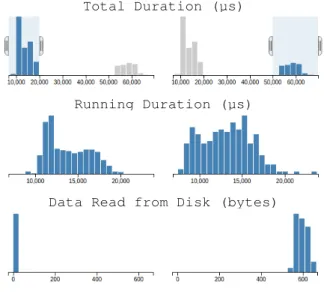
The aim of the filters is to allow the user to define two groups of executions to compare. They are presented as two columns of histograms. Each column is associated with a group of executions and each row is associated with a metric. Hence, each histogram shows the distribution of a metric within a given group. Initially, both columns are identical because all executions are included in both groups. To filter the executions of a group, the user selects a region on an histogram 4_{. For example, in Fig. 5, the left} group contains executions with a total duration under 20 ms while the right group contains executions with a total duration above 50 ms. It is possible to set as many filters as desired.

Whenever a filter is added to a metric, the histograms of the other metrics are updated to only take into account the executions that belong to their group. This can reveal interesting correlations between metrics. For example, Fig. 5 shows a case where the CPU time of an execution is not correlated with its total duration, but is correlated with the number of bytes read from the disk.

3.4.2 Flame Graph

Differential flame graphs were introduced in section 2.3 as a way to compare two CPU profiles. The second part of our comparion view reuses this visualization tool, but with some adaptations.

4. The implementation is inspired from http://square.github.io/ crossfilter/.

Total Duration (µs)

Running Duration (µs)

Data Read from Disk (bytes)

Fig. 5. Comparison Filters

First, our differential flame graphs are built from ECCTs instead of from CPU profiles. Fig. 6 shows that they can reveal latencies caused by chains of blocked threads and long disk requests. This is impossible with a simple CPU profile.

Second, our differential flame graphs are used to com-pare two groups of executions instead of two individual executions. The width of a box is proportional to the mean time spent in a calling context for executions of the right group. The hue of a box is computed from the number of standard deviations between mean times spent in a calling context in the two compared groups. This technique pre-vents colors to be applied to boxes in the presence of normal variations, which is a limitation of the original differential flame graphs.

Our differential flame graph is dynamically updated when filters are applied in the top part of the view.

main HandleRequest(int) FunctionA() FunctionB() FunctionC() FunctionD() [wait thread] OtherThread() sys:read [wait disk] Transition between threads

Fig. 6. Differential Flame Graph

3.4.3 List of executions

The bottom of the view presents two tables with the source trace and timestamp of a few executions sampled from the two compared groups. This data enables the user to find ex-ecutions of interest in another viewer such as TraceCompass to analyze the precise ordering of events.

3.4.4 Filtering algorithm

TraceCompare uses a map-reduce algorithm to update his-tograms when filters are modified. "Map" functions are applied to all executions that are either added to or removed from a group following a filter modification. The functions

determine in which bucket, of each histogram, affected exe-cutions belong. "Reduce" functions compute the new value of each histogram bucket.

A sorted index is kept for all metrics on which filters can be applied. Also, a filter is always specified as a range of accepted values for a given metric. Therefore, to update a filter, we simply find the first affected execution in the index and we traverse subsequent executions until we find the last affected one. This operation is performed in O(logN + M ) time, where N is the total number of executions and M the number of affected executions.

The user updates filters by dragging a handle on a histogram. Therefore, M is typically small at each mouse event and the views are updated quickly. The update takes a little bit more time when a lot of executions have a similar value for the filtered metric and are affected simultaneously. To keep the views responsive in that case, we could precom-pute the result of the reduction for segments of fixed size on each dimension.

TraceCompare uses the Crossfilter5 _{implementation of} this map-reduce algorithm. The algorithm has already been used to analyze multi-dimensional data sets of payment, meteorological and transportation data, but never to com-pare software performance metrics.

4

C

ASE

S

TUDIES

This section presents four performance problems, encoun-tered in real applications, along with a description of how TraceCompare can diagnose them. The first two case studies were made on test applications that we built to closely reproduce problems found in enterprise software. The two subsequent case studies show how TraceCompare was used to find real performance problems in MongoDB6_{, an} open-source database software.

4.1 CPU Contention in a Real-Time Application 4.1.1 Problem Summary

A realtime task is scheduled to be executed at a frequency of 100 Hz. Another task of higher priority (set with nice) is scheduled to be executed at a frequency of 30 Hz on the same CPU. At regular interval, the deadline of the second task occurs while the first task is running, increasing its execution time. Unfortunately, the developers are not aware of the existence of the second task.

4.1.2 Diagnosis

TraceCompare was used to compare slow executions of the first task against fast ones. The flame graph, partially reproduced in Fig. 7, immediatly revealed that the first task was preempted by the second during the slow executions. More interestingly, it showed call stacks from the second task. With these call stacks, it was clear where to look in the code to fix the problem. Without call stack events, the analysis tool could only have shown the name of the task that stole the CPU from the first task. Since threads are named after their parent, unless efforts are made to give

5. https://github.com/square/crossfilter 6. https://www.mongodb.org

them meaningful names, further investigation would have been needed to find out what was the purpose of the second task. [thread] [wait cpu] [thread] start_thread ImportantWork() start_thread AnnoyingWork() Stack of second task (preempting) Stack of first task (preempted) Preemption

{

{

}

... ...

Fig. 7. Differential Flame Graph Showing CPU Contention in a Real-Time Application

The histogram showing the "timestamp" metric of slow executions also provides useful information: it reveals that the problem is occurring at regular intervals.

4.2 Disk Contention in a Server Application 4.2.1 Problem Summary

A server has to read data from the disk to fulfill requests. At regular intervals, a request is about 5 times slower than usual.

4.2.2 Diagnosis

TraceCompare revealed that the additional latency found in the slow requests came from abnormaly long read() system calls. With a tool whose scope is limited to a single process, it would have been hard to pursue the analysis further. Fortunately, TraceCompare was able to leverage the information from a trace of the whole system to show precisely which other threads used the disk during these long system calls and what were their call stacks.

TraceCompare highlighted a single thread that always used the disk during the slow executions, but never dur-ing the fast executions. That thread was performdur-ing an fsync()system call after having written to a log file. With this information, fixing the problem was straightforward. 4.3 Lock Contention in MongoDB

4.3.1 Problem Summary

A client application generates data and inserts it into a MongoDB database (version 2.5.4). Most of the time, the whole operation takes around 10 ms. However, a fraction of the time, the operation takes more than 100 ms. Data is generated at less than 1 MB/s.

4.3.2 Diagnosis

The database insertions were performed serially, so it was unlikely that the performance variation was due to CPU or lock contention. Also, the MongoDB’s documentation states that insert operations don’t wait for data to be committed on disk before returning (a dedicated command is available to wait for that). Therefore, we didn’t expect disk latency to affect the performance of our application. Note that if our application had produced data at a higher rate, it would have been understandable that MongoDB throttled new insertions to flush its memory buffers.

The differential flame graph of TraceCompare, partially reproduced in Fig. 8, revealed that slow executions had

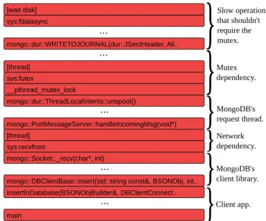
waited for a mutex protecting access to a list of pending changes. During these wait times, the mutex was held by a journalization thread. This information alone doesn’t lead to an obvious fix and could have been found by lock analysis with a tool such as Intel® VTune™7. However, TraceCom-pare sets itself apart from other tools by also revealing a function running on the journalization thread for almost all of the wait time. We analyzed the code of this function and discovered that it was not using the list protected by the mutex. Therefore, we wrote a simple patch to release the mutex before calling the costly function. We verified that the patch correctly fixed the serious performance problem that we had uncovered and we submitted it to the MongoDB developers. All this was done without any prior knowledge of the MongoDB codebase.

main

InsertInDatabase(BSONObjBuilder&, DBClientConnect.. mongo::DBClientBase::insert(std::string const&, BSONObj, int.. mongo::Socket::_recv(char*, int) sys:recvfrom [thread] mongo::PortMessageServer::handleIncomingMsg(void*) mongo::dur::ThreadLocalIntents::unspool() __pthread_mutex_lock sys:futex [thread] mongo::dur::WRITETOJOURNAL(dur::JSectHeader, Ali.. sys:fdatasync [wait disk] ... ... ... ... ...

}

}

}

}

}

}

Client app. MongoDB's client library. Network dependency. MongoDB's request thread. Mutex dependency. Slow operation that shouldn't require the mutex.

Fig. 8. Differential Flame Graph Showing a Lock Contention in MongoDB This diagnosis was made with an unmodified MongoDB binary. We only inserted probes in our client application to delimit the task to analyze. To track the latency, from our client application to the journalization thread of Mon-goDB, TraceCompare had to match TCP packets exchanged between both applications, and to analyze wake-up events within the Linux kernel.

4.4 Sleep in MongoDB 4.4.1 Problem Summary

Batch insert commands are sent to a MongoDB server (ver-sion 3.0.0 rc 10, WiredTiger storage engine). The commands are run in less than 700 µs most of the time. However, about 1 in 10 000 commands takes between 3 and 5 seconds to complete.

4.4.2 Diagnosis

TraceCompare made it easy to compare a group of fast exe-cutions against a group of slow exeexe-cutions. The comparison revealed that there was in fact two distinct sources of latency in our test scenario. Some executions were waiting for the

disk within pwrite64() system calls while other were blocked by a timer. Since disk contention can be expected when a lot of data is inserted in a database, we decided to create a second filter to focus on the more suspicious timer contention.

The flame graph showed that the timer contention was caused by a sleep within a function responsible to obtain a hazard pointer to a page of data. We located the sleep call in the source code. It was accompagnied by a comment explaining that if another thread was trying to evict the page from the cache at the same time, it was necessary to wait a while before retrying to obtain the pointer.

TraceCompare didn’t show any dependant work being done during the long sleeps. In fact, we were able to confirm that both the CPU and disk activity were very low during the sleeps, by using the information provided in the tables at the bottom of the view to locate the slow executions in another trace analysis tool. At that point, we were confident that we had found a synchronization bug in MongoDB, along with a precise diagnostic.

Despite the fact that the sleeps caused huge delays, they didn’t account for a significant proportion of the trace. They wouldn’t have caught our attention if we had used a profiler, which only shows global statistics. Having the ability to create groups of executions using multiple custom filters was a key feature to diagnose this problem. Also, having a trace of timestamped events allowed us to obtain resource usage statistics for specific time ranges.

5

P

ERFORMANCE

A

NALYSIS

We conducted experiments to evaluate the tracing overhead of our solution as well as the time required to analyze a trace in order to build a database of executions. It is crucial to be able to record all the events required by TraceCompare with low overhead. Indeed, it is unlikely that our solution would be used on production systems if it decreased perfor-mance noticeably. Rare bugs that occur under very specific conditions would therefore be out of its reach. Also, having a low overhead ensures that the behavior captured in the trace is similar to that of the uninstrumented system. On the other hand, a fast analysis time helps system administrators respond to problems quickly.

5.1 Environment

All experiments were run on a computer with a quad-core Intel® Core™ i7-3770 CPU running at 3.4 GHz, 16 GB of DDR3 memory and a 7200 RPM hard drive. The frequency scaling governor of the CPU was set to “performance” to ensure that it always runs at its maximum frequency. The Linux kernel version was 3.13.0-49 while the LTTng version was 2.6.0.

5.2 Cost of Tracing

We wanted to measure the overhead incurred by each step of the generation of our new syscall_stack event. To do so, we first created a microbenchmark that invokes the getpid() system call 100 million times and we timed its completion time when different parts of our kernel mod-ule were enabled. We repeated each experiment 20 times

and always got a standard deviation of less than 0.5%. The getpid() system call was chosen because of the low variability of its duration.

Registering empty probes to tracepoints located at the entry and exit of system calls incurs a cost of 96 ns per system call. This is because the Linux kernel has to go through a slow path whenever there are probes registered to system call tracepoints. Adding our code to detect long system calls in the probes brings an additionnal cost of 42 ns. These costs apply to all system calls, even those that turn out to be faster than the threshold for long system calls. When a long system call is detected, a signal is sent to the application so that it captures its call stack. Sending the signal and executing an empty signal handler takes 1.2 µs.

Next, we microbenchmarked the operations executed within the signal handler. We used microbenchmarks that repeat the measured operation 100 million times. We re-peated each experiment 20 times and always got a standard deviation of less than 2%.

The total time to unwind the stack depends on the number of frames currently on the stack. If it’s the first time that a stack frame is encountered, it takes 326 ns to process it. This is 20% faster than without our custom optimizations. Because decoded unwinding rules are cached, subsequent processing of the same stack frame takes only 7 ns. There is also a base cost between 30 ns and 700 ns, depending on whether all stack frames are handled by cached rules. Once a stack has been captured, it is written in an LTTng buffer, an operation that requires 175 ns.

cpu_stack events are generated from a signal sent at the expiration of a timer. Enabling the timer has a negligible overhead. The execution of the signal handler takes the same time as for syscall_stack events.

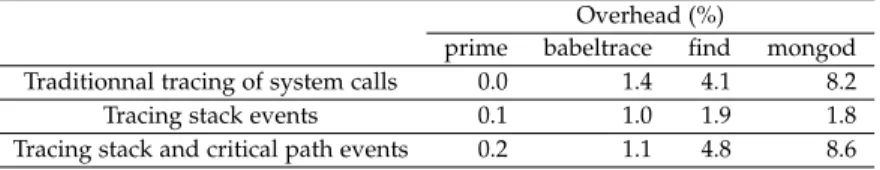
Finally, we wanted to determine how our instrumenta-tion affects typical applicainstrumenta-tions. Table 1 shows the time re-quired to run 4 programs under different tracing scenarios. The overhead in percentage is reported in Table 2. Each test case was run 100 times.

The "Traditional tracing of system calls" scenario is a baseline to compare with the "Tracing stack events" scenario. Indeed, our custom syscall_stack event reveals long system calls with a significatively lower cost than the tra-ditionnal system call events. TraceCompare requires a trace recorded under the "Tracing stack and critical path events" scenario.

prime is an application that computes a list of prime numbers up to 10 000. It does no system calls, so the overhead is mostly due to the statistical CPU profiling. babeltrace is a single-threaded program that reads CTF traces. It does a lot of system calls to open trace files and output results, but few of them are long enough to trigger the generation of a stack event. The 1% overhead is mostly due to the kernel module tracking the duration of each system call. find is a command-line tool that searches files recursively in the file system. It spends most of its time blocked on block device requests. Each request generates interrupts and context switches, which contribute to the 5% overhead of tracing critical path events. mongod is an open-source database server. It was tested using the client ap-plication presented in section 4.3. The interactions between

TABLE 1

Execution Time of Test Programs (in seconds)

prime babeltrace find mongod

Mean Dev. Mean Dev. Mean Dev. Mean Dev.

Base 9.11 0.00 17.57 0.17 14.39 0.18 9.91 0.28

Traditionnal tracing of system calls 9.11 0.00 17.81 0.14 14.99 0.28 10.72 0.06 Tracing stack events 9.12 0.00 17.74 0.15 14.67 0.35 10.09 0.20 Tracing stack and critical path events 9.13 0.00 17.76 0.15 15.08 0.30 10.76 0.05

TABLE 2 Overhead of Tracing

Overhead (%)

prime babeltrace find mongod Traditionnal tracing of system calls 0.0 1.4 4.1 8.2

Tracing stack events 0.1 1.0 1.9 1.8

Tracing stack and critical path events 0.2 1.1 4.8 8.6

multiple threads through synchronization primitives and TCP packets explain the 9% overhead.

5.3 Cost of the Analysis

The time required to build the database of executions for each of the case studies presented earlier is reported in Table 3. This metric is correlated with the size of the trace rather than its duration. It is always less than 3 times the time required to read the trace with babeltrace8 (a tool that just decodes the events of a trace).

The table also shows that the size of the generated database is on average 10% of the size of the source trace. Yet, it contained enough information to perform the precise diagnosis that we presented earlier. By keeping a database of executions rather than voluminous traces, system ad-ministrators could save storage space without sacrificing the convenience of being able to analyze the behavior of a system over a long period of time.

TABLE 3 Cost of the Analysis

Trace Database

Recording Time Size (MB) Build Time Size (MB)

4.1 13 min 26 s 52 17 s 7

4.2 22 min 42 s 86 20 s 7

4.3 2 min 38 s 31 7 s 3

4.4 5 min 11 s 129 32 s 13

6

F

UTURE

W

ORK

Our comparison tool has hard-coded rules to identify la-tencies caused by dependencies between threads, (provided that they use OS level synchronization), or by CPU or disk contention. Its scope could be widened by adding logic to account for GPU contention, CPU contention across virtual machines, or userspace synchronization through standard libraries. It is however impossible to handle out of the box the specificities of each application (e.g. custom task queues,

8. http://git.efficios.com/?p=babeltrace.git

custom IPC through shared memory). The declarative lan-guage used for trace analysis in [28] could be extended to allow the expression of these specificities.

We used TraceCompare to analyze performance regres-sions between multiple verregres-sions of the same program. Re-named functions can easily be dealt with by allowing the user to provide a file, mapping old function names to new names. However, the biggest challenge comes from major code refactoring, during which functions can be splitted or merged. Static analysis techniques exist to identify cloned syntactic blocks between multiple source files [29]. Tech-niques also exist to retrieve a mixed stack of function calls and syntactic blocks for a thread [30]. These techniques could be combined to allow a meaningful comparison be-tween traces recorded on different versions of the same program, even after a major refactoring.

Our userspace tracing library can only capture the stack for ELF binaries. It should be extended to properly handle programs written in a dynamic language and JIT compiled. It would also be useful to allow userspace processes to associate metrics with the current execution (e.g. number of returned results). Filters on these metrics could then be used to specify the execution groups to compare with more granularity.

7

C

ONCLUSION

In this paper, we presented a new tool that facilitates the detection and diagnosis of performance variations between multiple executions of the same task. A novel technique was proposed to capture the userspace stack of programs at key moments. The stacks were recorded along with kernel events using the LTTng tracer. We showed how to combine all these events to generate a database of ECCTs, a new data structure to describe latency that occurs at multiple levels during task executions. Then, we introduced an intuitive GUI that allows a user to specify groups of executions, using custom filters, in order to visualize their differences. An efficient map-reduce algorithm makes the views responsive, and userspace stacks make it easy to find the source code associated with identified differences. We detailed how our tool was able to discover performance bugs commonly

found in enterprise software and in MongoDB, a popular open-source software. Finally, we showed that the overhead of tracing the events, required by our comparison analysis, is always under 9%, which means that our solution can be used on production systems.

A

CKNOWLEDGMENT

This work was made possible thanks to the financial sup-port of Ericsson and the Natural Sciences and Engineering Council of Canada (NSERC).

R

EFERENCES

[1] I. Ceaparu, J. Lazar, K. Bessiere, J. Robinson, and B. Shneiderman, “Determining causes and severity of end-user frustration,” Inter-national Journal of Human-Computer Interaction, vol. 17, no. 3, pp. 333–356, 2004.

[2] E. Nygren, R. K. Sitaraman, and J. Sun, “The akamai network: A platform for high-performance internet applications,” SIGOPS Operating Systems Review, vol. 44, no. 3, pp. 2–19, Aug. 2010. [3] L. Adhianto, S. Banerjee, M. Fagan, M. Krentel, G. Marin, J.

Mellor-Crummey, and N. R. Tallent, “Hpctoolkit: tools for performance analysis of optimized parallel programs,” Concurrency and Com-putation: Practice and Experience, vol. 22, no. 6, pp. 685–701, Apr. 2010.

[4] A. Montplaisir-Gonçalves, N. Ezzati-Jivan, F. Wininger, and M. R. Dagenais, “State history tree: an incremental disk-based data structure for very large interval data,” in International Conference on Social Computing. IEEE, September 2013, pp. 716–724. [5] N. Ezzati-Jivan and M. R. Dagenais, “A framework to compute

statistics of system parameters from very large trace files,” SIGOPS Operating Systems Review, vol. 47, no. 1, pp. 43–54, Jan. 2013. [6] F. Giraldeau and M. R. Dagenais, “Approximation of critical path

using low-level system events,” to be published.

[7] D. J. Dean, H. Nguyen, X. Gu, H. Zhang, J. Rhee, N. Arora, and G. Jiang, “Perfscope: Practical online server performance bug inference in production cloud computing infrastructures,” in Proceedings of the ACM Symposium on Cloud Computing, ser. SOCC ’14. New York, NY, USA: ACM, 2014, pp. 1–13.

[8] B. H. Sigelman, L. A. Barroso, M. Burrows, P. Stephenson, M. Plakal, D. Beaver, S. Jaspan, and C. Shanbhag, “Dapper, a large-scale distributed systems tracing infrastructure,” Google research, 2010.

[9] Performance profiling with the timeline. [Online]. Available: https://developer.chrome.com/devtools/docs/timeline

[10] F. Rajotte and M. R. Dagenais, “Real-time linux analysis using low-impact tracer,” Advances in Computer Engineering, vol. 2014, June 2014.

[11] B. Gregg. (2014, November) Differential flame graphs. [Online]. Available: http://www.brendangregg.com/blog/ 2014-11-09/differential-flame-graphs.html

[12] D. Lee, S. Cha, and A. Lee, “A performance anomaly detection and analysis framework for dbms development,” IEEE Transactions on Knowledge and Data Engineering, vol. 24, no. 8, pp. 1345–1360, Aug. 2012.

[13] N. Joukov, A. Traeger, R. Iyer, C. P. Wright, and E. Zadok, “Op-erating system profiling via latency analysis,” in Proceedings of the 7th Symposium on Operating Systems Design and Implementation, ser. OSDI ’06. Berkeley, CA, USA: USENIX Association, 2006, pp. 89–102.

[14] P. E. McKenney, “Differential profiling,” in Proceedings of the Third International Workshop on Modeling, Analysis, and Simulation of Com-puter and Telecommunication Systems, 1995 (MASCOTS’95). IEEE, 1995, pp. 237–241.

[15] J. Trumper, J. Dollner, and A. Telea, “Multiscale visual compari-son of execution traces,” in IEEE 21st International Conference on Program Comprehension (ICPC), May 2013, pp. 53–62.

[16] C. H. Kim, J. Rhee, H. Zhang, N. Arora, G. Jiang, X. Zhang, and D. Xu, “Introperf: Transparent context-sensitive multi-layer performance inference using system stack traces,” SIGMETRICS Performance Evaluation Review, vol. 42, no. 1, pp. 235–247, June 2014.

[17] M. Weber, R. Brendel, and H. Brunst, “Trace file comparison with a hierarchical sequence alignment algorithm,” in IEEE 10th International Symposium on Parallel and Distributed Processing with Applications (ISPA), Leganés, Madrid, Spain, July 2012, pp. 247– 254.

[18] A. Hamou-Lhadj, S. S. Murtaza, W. Fadel, A. Mehrabian, M. Cou-ture, and R. Khoury, “Software behaviour correlation in a re-dundant and diverse environment using the concept of trace abstraction,” in Proceedings of the 2013 Research in Adaptive and Convergent Systems, ser. RACS ’13. New York, NY: ACM, 2013, pp. 328–335.

[19] S. Ghemawat. (2010, June) Google perftools cpu profile. [Online]. Available: http://google-perftools.googlecode.com/svn/trunk/ doc/cpuprofile.html

[20] kernel.org. (2014, June) perf: Linux profiling with performance counters. [Online]. Available: https://perf.wiki.kernel.org/ [21] J. Oakley and S. Bratus, “Exploiting the hard-working dwarf:

Trojan and exploit techniques with no native executable code,” in Proceedings of the 5th USENIX Conference on Offensive Technologies, ser. WOOT’11. Berkeley, CA, USA: USENIX Association, 2011, p. 11.

[22] F. Nybäck, “Improving the support for arm in the igprof profiler,” Master’s thesis, Aalto University, Oct. 2014.

[23] J. Olsa. (2012, May) perf: Add backtrace post dwarf unwind. [Online]. Available: http://lwn.net/Articles/499116/

[24] G. Ammons, T. Ball, and J. R. Larus, “Exploiting hardware per-formance counters with flow and context sensitive profiling,” in Proceedings of the ACM SIGPLAN 1997 Conference on Programming Language Design and Implementation, ser. PLDI ’97. New York, NY, USA: ACM, 1997, pp. 85–96.

[25] X. Zhuang, S. Kim, M. i. Serrano, and J.-D. Choi, “Perfdiff: A framework for performance difference analysis in a virtual ma-chine environment,” in Proceedings of the 6th Annual IEEE/ACM International Symposium on Code Generation and Optimization. New York, NY: ACM, 2008, pp. 4–13.

[26] M. Desnoyers and M. R. Dagenais, “The lttng tracer: A low impact performance and behavior monitor for gnu/linux,” in Ottawa Linux Symposium, Ottawa, Ontario, 2006, pp. 209–224.

[27] S. Rostedt, “Using the trace_event() macro,” http://lwn.net/ Articles/379903/, mars 2010, consulté le 26 janvier 2015. [28] F. Wininger, “Conception flexible d’analyses issues d’une trace

système,” Master’s thesis, École Polytechnique de Montréal, Apr. 2014.

[29] E. Merlo and T. Lavoie, “Computing structural types of clone syntactic blocks,” in 16th Working Conference on Reverse Engineering, 2009. WCRE ’09, Oct. 2009, pp. 274–278.

[30] N. R. Tallent, J. M. Mellor-Crummey, and M. W. Fagan, “Binary analysis for measurement and attribution of program perfor-mance,” SIGPLAN Notices, vol. 44, no. 6, pp. 441–452, June 2009.

François Doray received the BEng degree in Software Engineering

and MS degree in Computer Engineering from École Polytechnique de Montréal. He is a software developer at Google in Montreal, Canada (effective in August, 2015). His research interests include performance analysis tools and parallel systems.

Michel Dagenais is a professor at École Polytechnique de Montreal,

in the Computer and Software Engineering Department. His research interests include several aspects of multicore distributed systems with emphasis on Linux and open systems. His group has made several original contributions to Linux.