Parallel seed-based approach to multiple protein structure similarities detection

HAL Id: hal-01093809

https://hal.inria.fr/hal-01093809

HAL is a multi-disciplinary open access archive for the deposit and dissemination of sci-entific research documents, whether they are pub-lished or not. The documents may come from

L’archive ouverte pluridisciplinaire HAL, est destinée au dépôt et à la diffusion de documents scientifiques de niveau recherche, publiés ou non, émanant des établissements d’enseignement et de

Parallel seed-based approach to multiple protein

structure similarities detection

Guillaume Chapuis, Mathilde Le Boudic-Jamin, Rumen Andonov, Hristo

Djidjev, Dominique Lavenier

To cite this version:

Guillaume Chapuis, Mathilde Le Boudic-Jamin, Rumen Andonov, Hristo Djidjev, Dominique Lavenier. Parallel seed-based approach to multiple protein structure similarities detection . 2014. �hal-01093809�

Parallel seed-based approach to multiple

protein structure similarities detection

∗

Guillaume Chapuis

_{Mathilde Le Boudic - Jamin}

Rumen Andonov

_{Hristo Djidjev}

_{Dominique Lavenier}

October 4, 2014

Abstract

Finding similarities between protein structures is a crucial task in molecular biology. Most of the existing tools require proteins to be aligned in order-preserving way and only find single alignments even when multiple similar regions exist. We propose a new seed-based ap-proach that discovers multiple pairs of similar regions. Its computa-tional complexity is polynomial and it comes with a quality guarantee– the returned alignments have both Root Mean Squared Deviations (coordinate-based as well as internal-distances based) lower than a given threshold, if such exist. We do not require the alignments to be order preserving (i.e. we consider non-sequential alignments), which makes our algorithm suitable for detecting similar domains when com-paring multi-domain proteins as well as to detect structural repetitions within a single protein. Because the search space for non-sequential alignments is much larger than for sequential ones, the computational burden is addressed by extensive use of parallel computing techniques: a coarse-grain level parallelism making use of available CPU cores for computation and a fine-grain level parallelism exploiting bit-level con-currency as well as vector instructions.

Key words: protein structure comparison, alternative align-ments, alignment graph, maximal clique, Streaming SIMD Extensions (SSE), bit-level parallel computations

∗_{Preliminary version of this work was presented at PPAM 2013} †_{INRIA/IRISA and University of Rennes 1, France}

1

Introduction

A protein’s three dimensional structure tends to be evolutionarily better pre-served than its sequence. Therefore, finding structural similarities between two proteins can give insights into whether these proteins share a common function or whether they are evolutionarily related. Structural similarity between two proteins is usually defined by two functions – a one-to-one map-ping (also called alignment or correspondence [12]) between two subchains of their three dimensional representations and a specific scoring function that assesses the alignment quality. The structural alignment problem is to find the mapping that is optimal with respect to the scoring function. Hence, the complexity of the protein structural alignment problem and the quality of the found solution strongly depend on the way that scoring function is defined.

The most commonly used among the various measures of alignment simi-larity are the internal-distances root mean squared deviation (RMSDd) and

the coordinate root mean squared deviation (RMSDc) (see (3) and (2)

re-spectively for the exact definitions). Tightly related to these measures are the two main approaches for solving the structural alignment problem. The similarity score in the first approach is based on the internal distances matrix, where a set of distances between elements in the first protein is matched with a set of distances in the second protein. The second approach uses the actual Euclidean distances between corresponding atoms in two proteins and aims to determine the rigid transformation that superimposes the two structures. A huge majority of the algorithms representing these approaches are heuristics [7, 20, 27, 32, 33] (excellent reviews can be found in refs. [10, 18]) and as such, do not guarantee finding an optimal alignment with respect to any scoring function. The fact that finding exact solutions in this field is computationally hard is related to the fact that computing the longest align-ment of protein structures is typically modeled as an NP-hard problem, e.g., the protein threading problem [16], the problem of enumerating all maximal cliques [5, 26], or finding a maximum clique [13, 19, 28].

These results have been generalized by Kolodny and Linial [12], who showed that protein structural alignment is NP-hard if the similarity score is distance based. They also point out that a correct and efficient solution of the structural-alignment problem must exploit the fact that the proteins lie in three-dimensional Euclidean space.

in-tractabilities pointed out in [12]. Our algorithm is both internal-distances based and Euclidean-coordinates based (i.e., it uses a rigid transformation to optimally superimpose the two structures). Its computational complexity is polynomial and it comes with a quality guarantee – for a given threshold

τ, it guarantees to return alignments that have RMSDc as well as RMSDd

less than 2τ, if such exist.

Our algorithms is motivated by a class of exact structural-alignments algorithms that look for the largest clique in the so-called product (or align-ment) graphs [13, 19, 28]. The edges in such graphs encode information about pairs of residues in the two proteins that match based on internal distances between them, namely, if the difference between corresponding distances does not exceed some fixed parameter τ. Then a clique of size k would correspond to subsets of k residues in both proteins that match.

Here, we relax this condition and accept cliques such that edges cor-respond to matching of similar internal distances up to 2τ. For this re-laxed problem, we propose a polynomial algorithm that takes advantage of internal-distance similarities among both proteins to search for an optimal transformation to superimpose their structures. We also replace the goal of finding the largest clique by the one of returning several very dense "near-clique" subgraphs. This choice is strongly justified by the observation that distinct solutions to the structural-alignment problem that are close to the optimum are all equally viable from the biological perspective, and hence are all equally interesting from the computation standpoint [2, 12].

To the best of our knowledge, our tool is unique in its capacity to gener-ate multiple alignments with “guaranteed good” both RMSDc and RMSDd

values. We do not require the alignments to be order preserving which makes our algorithm suitable for detecting similar domains when comparing multi-domain proteins. Thanks to this property, the tool is able to find both sequential and non-sequential alignments, as well to detect structural repe-titions within a single protein and between related proteins.

However, to enumerate exhaustively multiple similar regions requires a more systematic approach than those developed in other existing heuristic-based tools. The computational burden is addressed by extensive use of parallel computing techniques: a coarse grain level parallelism making use of available CPU cores for computation and a fine grain level parallelism exploiting bit-level optimization as well as vector instructions.

Other non-sequential structure alignment methods have been recently proposed (excellent review on this topic can be found in the very recent

reference [21]). None of them is close to the approach proposed here. As they are all heuristic and do not guarantee finding an optimal alignment, a detailed comparison with algorithms based on different concepts requires extensive numerical experiments and is outside the scope of this study.

Here we present a significantly improved and expanded version of a paper originally presented at the PPAM 2013 conference [3]. In comparison to [3], the current version contains detailed description and explanation of all steps of the algorithms, all pseudo codes, supplementary figures illustrating the algorithms and the experimental results, and extended reference section. Additional sections are added including a comparison between the straight-forward and the bit-vector implementations based on complexity analysis as well as detailed analysis of the work from the point of view of future performance improvements and additional possible applications.

2

Preliminaries

2.1

Measures for protein alignments

Consider a protein P of n atoms, P = (p1, . . . , an), with pi ∈ R3. Many

measures have been proposed to assess the quality of a protein alignment. These measures include additive scores based on the distance between aligned residues such as the TM-score [34], the DALI score [8, 30], the PAUL score [31] and the STRUCTAL score [29] and Root Mean Square Deviation (RMSD) based scores, such as RMSD100, SAS and GSAS [11]. Given a set of n devi-ations S = s1, s2, ..., sn, its Root Mean Square Deviation is

RM SD(S) = v u u t 1 n n X i=1 s2_i. (1)

Two different RMSD measures are used for protein structure comparison. The first one, RMSDc, takes into account deviations consisting of the

eu-clidean distances between matched residues after optimal superposition of the two structures and is defined as

RM SDc(P ) = min ˆ P v u u t 1 n n X i=1 (pi−pˆi)2. (2)

The second one, denoted here by RMSDd, takes into account deviations

consisting of absolute differences of internal distances within the matched structures. The measured deviations are |d(i, j)−d(k, l)|, for all couples of matching pairs “i ↔ k, j ↔ l.” Let M be the latter set and Nm, its

cardinal-ity. We have that

RM SDd(M) = v u u t 1 Nm X (ij,kl)∈M (|d(i, j)−d(k, l)|2_{). (3)}

2.2

Alignment graphs

An undirected graph G = (V, E) is represented by a set V of vertices and a set E of edges between these vertices. In this paper, we focus on a subset consisting of grid-like graphs, referred to as alignment graphs.

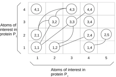
An m × n alignment graph G = (V, E) is a graph in which the vertex set

V is depicted by an m × n array T , where each cell T [i][k] contains at most one vertex (i, k) from V . An example of such an alignment graph for protein comparison is given in Figure 1.

A good matching of two proteins P1 and P2 can be found by analyzing

their alignment graph G = (V, E), where V = {(v1, v2) | v1 ∈ V1, v2 ∈ V2}

and V1 (resp. V2) is the set of atoms of interest in protein P1 (resp. protein

P2). A vertex (I, I′) is present in V only if atoms I ∈ V1 and I′ ∈ V2 are

compatible. An example of incompatibility could be different electrostatic properties of the two atoms. An edge ((I, I′), (J, J′)) is in E if and only if

the distance between atoms I and J in protein P1, d(I, J), is similar to the

distance between atoms I′ _{and J}′ _{in protein P}

2, d(I′, J′). In our case, these

distances are considered similar if |d(I, J) − d(I′

, J′)| < τ, where τ is a given

threshold.

We arbitrarily order the vertices of the alignment graph and assign a corresponding index to each of them. In subsequent sections, the notion of

successors of a vertex v refers to all the vertices that are adjacent to v in

the alignment graph and have a higher index than v with respect to those fixed indices. The notion of neighbors of a vertex v refers to the set of all the vertices that are adjacent to v in the alignment graph regardless of their respective indices. Formally, we define

successors(vi ∈ V) ={vj ∈ V |(vi, vj) ∈ E & i < j}

Atoms of interest in protein P₁ Atoms of interest in protein P₂ 1 2 3 4 1 2 3 4 5 1,1 2,1 4,1 4,3 3,3 3,2 1,2 1,4 2,4 3,4 4,4 2,5

Figure 1: Example of an alignment graph used here to compare the structures of two proteins. The presence of an edge between vertex (1, 1) and vertex (3, 2) means that the distance between atoms 1 and 3 of protein 1 is similar to the distance between atoms 1 and 2 of protein 2. The clique (2, 1) (3, 2) (4, 3) indicates that RMSDd of structures (2, 3, 4) and (1, 2, 3) is less than τ

[19].

In an alignment graph of two proteins P1 and P2, a subgraph with high

density of edges denotes similar regions in both proteins. One can, there-fore, find similarities between two proteins by searching in the corresponding alignment graph for subgraphs with high edge density. The highest possible edge density is found in a clique, a subset of vertices that are all connected to each other. Then a clique of size k would correspond to subsets of k residues in both proteins that match since all k(k−1)

2 internal distances are similar.

For these reason approaches like ProBis [13] and DAST [19] aim at finding the maximum clique in an alignment graph.

3

Methods

3.1

Our approach

Since finding a maximum clique in a graph is NP-hard and any exact solver faces prohibitively long run times for some instances, here we relax the above definition of clique and accept cliques such that edges correspond to matching

of similar internal distances up to 2τ. We also replace the goal of finding the largest clique by the one of returning several very dense "near-clique" subgraphs.

Our method uses geometric properties of the 3-d space. Instead of test-ing for the presence of all edges among a subset S of vertices, in order to determne if S defines a clique, we only test for the presence of edges between every vertex of the subset and an initial 3-clique (triangle), referred to as

seed. This reduction of the performed comparisons is crucial and leads to a

polynomial algorithm that takes advantage of internal-distance similarities among both proteins to search for an optimal transformation to superimpose their structures.

3.2

Overview of the algorithm

Algorithm 1 gives an overview of our approach. The algorithm consists of the following three steps:

• Seeds in the alignment graph are enumerated. In our case, a seed is a set of three points in the alignment graph that correspond to two triangles (one in each protein) with similar internal distances. This step is detailed in Section 3.3.

• Each seed is then extended. Extending a seed consists in adding all pairs of atoms, for which distances to the seed are similar in both proteins, to the set of three pairs of atoms that make up the seed. Seed extension is detailed in Section 3.4.

• Each seed extension is filtered - cf. lines 10 through 15. Extension filtering is detailed in Section 3.5 and consists in removing pairs of atoms that do not match correctly.

Filtered extensions are then ranked according to their size - number of aligned pairs of atoms - and a user-defined number of best matches are returned. This process is explained in Section 3.7. For very large align-ment graphs, the graph can be partitioned into a user-defined number of parts to speed up computations. The graph is partitioned using a min-cut type of heuristic to preserve the quality of the results. Each subgraph is then processed independently. This process is explained in Section 5. The overall worst-case complexity of the whole algorithm without partitioning is

Algorithm 1 Overview of the algorithm

1 f u n c t i o n find_alignments ( graph )

2 INPUT: graph , an alignment graph between atoms from two

p r o t e i n s 3 OUTPUT: r e s L i s t , a l i s t o f the l a r g e s t d i s t i n c t alignments found 4 5 R e s u l t L i s t r e s L i s t = e m p t y _ r e s u l t _ l i s t ( ) 6 S e e d L i s t s e e d s = enumerate_seeds ( graph ) 7 For each seed i n s e e d s

8 VertexSet s e t = extend_seed ( seed ) 9 VertexSet r e s u l t = empty_set ( ) 10 For each v e r t e x i n s e t 11 I f ( i s _ v a l i d ( v e r t e x ) ) 12 r e s u l t . add ( v e r t e x ) 13 End I f 14 r e s L i s t . i n s e r t _ i f _ b e t t e r ( r e s u l t ) 15 End For 16 End For

3.3

Seed enumeration

A seed consists of three pairs of atoms that form similar triangles in both proteins. A triangle IJK in protein P1 is considered similar to a triangle

I′

J′

K′ in protein P

2if the following conditions are met: |d(I, J)−d(I′, J′)| <

τ, |d(I, K) − d(I′_{, K}′)| < τ and |d(J, K) − d(J′_{, K}′)| < τ, where d denotes

the Euclidean distance and τ is a user-defined threshold parameter. The default value for τ is 2.0 Ångstroms.

In the alignment graph terminology, these conditions for a seed (vi =

(I, I′_{), v}

j = (J, J′), vk= (K, K′)) in graph G(V, E) translate to the following:

(vi, vj) ∈ E, (vi, vk) ∈ E and (vj, vk) ∈ E.

A seed thus corresponds to a 3-clique in the alignment graph; i.e., three vertices that are connected to each other. Enumerating all the seeds is there-fore equivalent to enumerating every 3-clique in the input alignment graph.

Not all 3-cliques, however, are relevant. Suitable 3-cliques are composed of triangles for which a unique transformation can be found to optimally

superimpose them. Namely, 3-cliques composed of triangles that appear to be too “flat” will not yield a useful transformation. We thus ensure that the triangles in both proteins defined by a potential seed are not composed of colinear points (or points which are close to being colinear). The method is detailed in Section 3. The worst-case complexity of this step is O(|E|3/2₎

using, e.g., the algorithms from [25].

Algorithm 2 Seed enumeration

1 f u n c t i o n enumerate_seeds ( graph )

2 INPUT : graph , an a l i g n m e n t graph between atoms from two

p r o t e i n s

3 OUTPUT: s e e d L i s t , a l i s t o f s u i t a b l e 3− c l i q u e s ( i . e .

t r i p l e t s o f v e r t i c e s t h a t a r e c o n n e c t e d t o each o t h e r and c o r r e s p o n d t o non−d e g e n e r a t e d t r i a n g l e s i n both

p r o t e i n s )

4

5 S e e d L i s t s e e d L i s t = empty_seed_list ( ) 6 For each v e r t e x 1 i n graph

7 For each v e r t e x 2 i n g e t _ s u c c e s s o r s ( v e r t e x 1 ) 8 For each v e r t e x 3 i n g e t _ s u c c e s s o r s ( v e r t e x 2 ) 9 I f i s _ e d g e ( v e r t e x 1 , v e r t e x 3 ) 10 I f c o l l i n e a r i t y _ c h e c k ( v e r t e x 1 , v e r t e x 2 , v e r t e x 3 ) 11 s e e d L i s t . add ( v e r t e x 1 , v e r t e x 2 , v e r t e x 3 ) 12 End I f 13 End I f 14 End For 15 End For 16 End For

3.4

Seed extension

Extending a seed consists in finding the set of vertices that correspond to pairs of atoms that potentially match well (see Section 3.5 for details) when the two triangles defined by the seed are optimally superimposed. Finding a superset of pairs of atoms that match well is performed by triangulation with the three pairs of atoms composing the seed. Let (vi = (I, I′), vj =

(J, J′_{), v}

k = (K, K′)) be a seed of an alignment graph G(V, E) as defined in

Section 3.3. Then the extension of the seed (vi, vj, vk) is defined as the set

extension(vi, vj, vk) ={vl = (L, L′)| |d(L, I) − d(L′ , I′_{)| < τ ∧} |d(L, J) − d(L′ , J′_{)| < τ ∧} |d(L, K) − d(L′ , K′_{)| < τ}.}

In the alignment graph terminology, the previous definition translates to: extension(vi, vj, vk) = neighbors(vi) ∩ neighbors(vj) ∩ neighbors(vk).

The detail of seed extension is given in Algorithm 3. The sequential compu-tational complexity associated to this step is O(|V |). For the complexity of our parallel implementation refer to subsection 4.3.

Algorithm 3 Seed extension

1 f u n c t i o n extend_seed ( vertexA , vertexB , vertexC )

2 INPUT: a seed r e p r e s e n t e d by t h r e e v e r t i c e s ( or p a i r s

o f atoms ) from the alignment graph

3 OUTPUT: res , a s e t o f p a i r s o f atoms that p o t e n t i a l l y

match w e l l when atoms from the seed are o p t i m a l l y superimposed ;

4 s i z e , the s i z e o f the r e t u r n e d s e t 5

6 BinaryVertexSet setA = get_neighbors ( vertexA ) 7 BinaryVertexSet setB = get_neighbors ( vertexB ) 8 BinaryVertexSet setC = get_neighbors ( vertexC ) 9 BinaryVertexSet tmp = i n t e r s e c t i o n ( setA , setB ) 10 BinaryVertexSet r e s = i n t e r s e c t i o n (tmp , vertexC ) 11 i n t s i z e = pop_count ( r e s )

3.5

Extension filtering

The triangulation performed when extending a seed is not sufficient to find alignments with good RMSD measures. Indeed, in most cases, knowing

the distance of a point in a three dimensional space to three other non-aligned points yields two possible locations. These locations are symmetrical with respect to the plane defined by the three reference points. A vertex in a seed extension represents a pair of atoms, one in each studied proteins. By construction, these atoms have similar distances to the three points of their respective triangles. It may happen that one of the two points, say L, is located, in protein P1, on one side of the plane defined by its reference

triangle, while the second point, say L′, in protein P

2, lies on the other side

of the plane defined by the two optimally superimposed reference triangles -see Figure 2.

Figure 2: Example of symmetry issues. Even though, vertex vl = (L, L′)

belongs to the extension of seed(vi, vj, vk), points L and L′ lie on different

sides of the plane defined by optimally superimposed triangles IJK and

I′

J′

K′.

Using quadruplets of vertices as seeds does improve the quality of seed extensions but greatly increases the computational cost of seed enumeration and degeneration check on the corresponding tetrahedra. Moreover, larger seeds do not completely ensure the quality of extensions. Namely, in cases where, for a vertex vl = (L, L′), atom L (resp. L′) is very distant from

atoms I, J and K (resp. atoms I′_{, J}′ _{and K}′_{) of a seed (v}

i = (I, I′), vj =

(J, J′), v

k = (K, K′)), distance similarities to the atoms of the seed do not

ensure similar positions of atoms L and L′ in the two proteins.

In order to remove issues with symmetry (where the atoms in the extend-ing pair are roughly symmetrical with respect to the plane determined by the seed atoms) and distance from the seed, we implement a method to filter seed

extensions. This method consists in computing the optimal transformation T to superimpose the triangle from the seed corresponding to the first protein onto the triangle corresponding to the second. The optimal transformation is obtained in constant time with respect to the size of the alignment by us-ing the fast, quaternion-based method of [17]. For each pair of atoms (L,L’) composing the extension of a seed (vi = (I, I′), vj = (J, J′), vk = (K, K′)),

we compute the Euclidean distance between T (L) and L′_{. If the distance}

is greater than a given threshold τ, the pair is removed from the extension. The filtering method is detailed in Algorithm 4. The complexity of this step is O(|V |) per seed.

Algorithm 4 Extension filtering algorithm

1 f u n c t i o n f i l t e r _ e x t e n s i o n ( e x t e n s i o n )

2 INPUT: e x t e n s i o n , a s e t o f p a i r s o f atoms

3 OUTPUT: r e s u l t , a s u b s e t o f the e x t e n s i o n c o n t a i n i n g

only p a i r s o f atoms that match w e l l

4

5 VertexSet r e s u l t = empty_set ( )

6 Matrix t r a n s f o r m a t i o n = get_optimal_transformation ( seed

)

7 For each v e r t e x i n e x t e n s i o n

8 Point L = g e t _ c o o r d i n a t e s _ i n _ f i r s t _ p r o t e i n ( v e r t e x ) 9 Point L_prime = get_coordinates_in_second_protein (

v e r t e x )

10 Point L_transformed = apply_transformation (L ,

t r a n s f o r m a t i o n )

11 Float d i s t a n c e = d i s t ( L_transformed , L_prime ) 12 I f ( d i s t a n c e < t h r e s h o l d )

13 r e s u l t . i n s e r t ( v e r t e x ) 14 End I f

15 End For

3.6

Guarantees on resulting alignments’ RMSD scores

By construction, the filtering method ensures that the RMSD for a resulting alignment is less than τ: the distance between two aligned residues after

superimposition of the two structures is guaranteed to be less than τ. Internal distances between any additional pair of atoms and the seed is also guaranteed, by construction to be less than τ. Concerning internal distances between two additional pairs of atoms, we show that in the worst possible case the difference does not exceed 2τ, see Figure 3. The worst possible case happens when two additional pairs of atoms vl = (L, L′) and

vm = (M, M′), added to the extension of a seed (vi, vj, vk), have atoms L,

L′, M and M′ aligned, after superimposition, and atoms from one protein

lie within the segment defined by the two other atoms. In such a case, the filtering step ensures that d(L, L′_{) < τ and d(M, M}′_{) < τ ; it follows that}

|d(L, M) − d(L′ , M′)| < 2τ. vi=(I , I ') vj=(J , J ') vk=(K , K ') vl= L, L'  vm= M , M ' d L, L'  d M , M '

Figure 3: Illustration of the guarantee on the similarity of internal distances between two pairs of atoms vl = (L, L′) and vm = (M, M′), here represented

in yellow, added to a seed (vi, vj, vk) represented in blue. Dashed lines

rep-resent internal distances, the similarity of which is tested in the alignment graph.

3.7

Result ranking

When comparing two proteins, we face a double objective: finding align-ments that have both long overlaps and low RMSD scores. The methodol-ogy described in Section 3.5 ensures that any returned alignment will have

a RMSDd lower or equal to twice the user-defined parameter τ. We can

therefore leave the responsibility to the user to define a threshold for RMSD scores of interest. However, ranking alignments that conform to this RMSD threshold simply based on their lengths is not an acceptable solution. In a given alignment graph, several seeds may lead to very similar transforma-tions and thus very similar alignments. The purpose of returning multiple alignments is to find distinct similar regions in both proteins. Therefore, when two alignments are considered similar, we discard the shorter of the two.

Two alignments are considered similar, when they share a defined number of pairs of atoms. This number can be adjusted depending on the expected length of the alignments or even set to a percentage of the smaller of the two compared alignments. This methodology of ranking results ensures that no two returned alignments match the same region in the first protein to the same region in the second protein.

3.8

Graph splitting

Large protein alignment graphs can contain millions of edges. In order to reduce the computations induced by such large graphs, a graph splitting scheme is implemented.

Graph splitting is performed using a min-cut like heuristic, also known as multi-level graph partitioning, provided by the METIS library [9]. This heuristic partitions the graph in k components of similar number of vertices and aims at minimizing the number of inter-component edges - edges between vertices that belong to distinct components. In order to further minimize the number of inter-component edges, we allow the sizes in terms of numbers of vertices of the components to vary up to an order of magnitude. The assumption is that such partitions will keep each area of interest in the graph within a single component.

Once a partition is obtained, subgraphs corresponding to the k compo-nents are sorted according to their respective numbers of vertices. Each sub-graph is then processed in decreasing order of sizes starting with the largest one. The list of best results is transmitted from one subgraph to another, in order to be able to discard seeds whose extensions are smaller than the best results found so far.

In practice, partitioning the graph tends to group vertices of each of the best results within a single component. However, several of these vertices

may be placed in different components. To address this issue, seeds yielding the best results in a subgraph are extended and filtered once more using atoms from the initial global graph.

This second extension and filtering phase significantly improves the length of resulting alignments but does not guarantee to provide the same results as without partitioning. However, experimental results show that a given graph could be partitioned in up to 10 components with only a 2% loss in terms of alignment length and a four fold overall speedup.

The graph splitting scheme is described in Algorithm 5.

Algorithm 5 Graph splitting algorithm

1 f u n c t i o n split_and_solve ( globalGraph )

2 INPUT: globalGraph , an alignment graph between atoms

from two p r o t e i n s

3 OUTPUT: globalRes , a l i s t o f the l o n g e s t d i s t i n c t

alignments found i n the graph

4

5 R e s u l t L i s t g l o b a l R e s = e m p t y _ r e s u l t _ l i s t ( ) 6 Graph [ ] subGraphs = s p l i t ( globalGraph ) 7 s o r t ( subgraphs )

8 For each subGraph i n subGraphs

9 S e e d L i s t best_seeds = empty_list ( )

10 S e e d L i s t s e e d s = enumerate_seeds ( subGraph ) 11 For each seed i n s e e d s

12 VertexSet c u r r e n t _ r e s = extend_and_filter (

subGraph , seed )

13 best_seeds . i n s e r t _ i f _ b e t t e r ( seed ) 14 End For

15 For each seed i n best_seeds

16 VertexSet c u r r e n t _ r e s = extend_and_filter (

globalGraph , seed )

17 g l o b a l R e s . i n s e r t _ i f _ b e t t e r ( c u r r e n t _ r e s ) 18 End For

4

Parallelism

4.1

Overview of the implemented parallelism

The overall computational complexity of our algorithm being O(|V | ∗ |E|3/2_),

handling large protein comparison with a decent level of precision - i.e., using alignment graphs with a large number of edges - can prove time-consuming. Our approach is however parallelizable at multiple levels.

Figure 4 shows an overview of our parallel implementation. Multiple seeds are treated simultaneously to form a coarse-grain level of parallelism, while a finer grain parallelism is used when extending a single seed.

nei ghbors i₁∩ nei ghbors j₁∩ nei ghbors k₁

seed₁i₁, j₁, k₁: Filtering

nei ghbors i2∩ nei ghbors j2∩ nei ghbors k2

seed2i2, j2, k2: Filtering

nei ghbors i_n∩ nei ghbors j_n∩ nei ghbors k_n seed_ni_n, j_n, k_n: Filtering . . . Coarse-grain parallelism Fine-grain parallelism Enumeration Extension

Figure 4: Overview of the implemented parallelism.

4.2

Coarse-grain parallelism

This level of parallelism is implemented using the open MP standard [4]. A user-defined number of threads is spawned to handle, in parallel, computa-tions for the seeds generated in the seed enumeration procedure.

In order to output only significant (sufficiently large) alignments we per-form here a kind of pruning strategy. It is based on the size of a seed extension which is in fact an easily computed upper bound of the alignment to be pro-duced by the given seed. Whenever this size is smaller than the length of any of the alignments present in the result list (those are the best alignments, so called records), the corresponding seed is discarded, thus avoiding the cost of a filtering step.

In this regard, our pruning strategy is similar to the one applied in a branch-and-bound (B&B) kind of algorithms. A sequential implementation of this strategy is relatively easy since there is only one list of records. The

order in which seeds (tasks to be performed) are treated, is crucial for the efficiency of the approach. As sooner as the best alignments are computed, more tasks can be discarded and many computations can be avoided. How-ever, parallelizing the approach induces the same challenges that parallel B&B implementations face [15] which can be resumed as follows.

Each thread has now its own (local) list of records which are only lower bounds of the global records found so far by all threads. The pruning strat-egy is less efficient and could even result in an increase of the amount of computations. One option to avoid this is to make threads share the list of records and to keep it updated. However, inserting frequently new entries in this global-result list, or often updating its content, would prove rather inefficient, because thread safety would need to be ensured by using locks around accesses to this result list. With such locks, threads would often stall whenever inserting a new alignment and the time lost on these accesses would only increase with the number of threads in use. In order to avoid any bottleneck when inserting a new alignment in the result list, in our im-plementation each thread has its own private list. These lists are merged at the end of the computations to form a final result list. This implementation choice prevent the need for a synchronization mechanism and allow threads to be completely independent.

4.3

Fine-grain parallelism

Seed extension makes extensive use of set intersection operations. We define for each vertex v a set set(v) containing all neighbors of v. Then, for each edge (v, w), the set of seeds containing (v, w) can be computed by finding the intersection of set(v) with set(w). In this section, we compare two alternative implementations for computing set intersection.

4.3.1 Straight-forward implementation

The straight-forward implementation of a set of vertices is to store in a sorted array the indices of the vertices that are present in the set. Computing the intersection of two such sets, S1 and S2, therefore consists in traversing

both arrays and adding common vertices to the resulting intersection. The complexity of such an approach is thus O(M + N), where M is the length of S1 and N is the length of S2. Once the intersection has been found, the

4.3.2 Bit-vector implementation

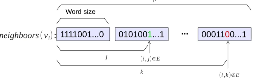
In order to speed up set intersection operations, we implemented a bit-vector representation of the neighbors set of each vertex of the alignment graph. To any vertex vi, we associate a vector neighbors(vi) where the bit at position

j is 1 if and only if vertexes vi and vj are connected in the alignment graph

(see Fig. 5 for illustration).

1111001...0 0101001...1 ... 0001100...1 Word size (i , j)∈E ∣V∣ (i ,k )∉E j k neighboors(v_i):

Figure 5: Bit-vector representation of the neighbors of vertex vi in an

align-ment graph G(V, E). In this example, vj unlike vk is a neighbor of vi.

This representation of the neighbors sets allows bit parallel computations of set intersection. A simple logic and operation over every word element of the two sets yields the intersection. For faster traversal of the neighbors set a traditional list representation is also kept. This list representation allows easy access to the first and the last elements of the neighbors set. Knowing the first and last elements of the sets allows to restrict the area of interest for intersection operations as described below. Let fi (resp. fj) be the first

non-zero bit in neighbors(vi) (resp. neighbors(vj)), while li (resp. lj) denote

the last non-zero bit in neighbors(vi) (resp. neighbors(vj)). We then apply

the logic and operator only over the interval [b, e] where b = max{fi, fj}and

e= min{li, lj}.

Intersection operations also benefit from SSE1 _{instructions. A number}

of atomic operations equal to the size of the SSE registers available on the machine (typically 128 or 256) can be computed simultaneously.

However, this bit-vector approach to computing set intersections increases the number of atomic operations to perform. Namely, vertices, which are not

1

neighbors of any of the two vertices for which the intersection is computed, will induce atomic operations; provided such vertices reside in the area of interest. Such vertices would not be considered in the first approach to set intersection.

In order to efficiently compute the size of the intersection in case of a bit-vector implementation, we use a built-in population count instruction (POPCNT) available in SSE4. This operation returns, in constant time, the number of bits set in a single machine word. For architectures without a built-in population count instruction, a slower yet optimized alternative is provided.

4.3.3 Straight-forward versus bit-vector implementations

As mentioned in section 4.3.1, the complexity of an intersection operation with the straight-forward implementation is in O(M + N), where M and N denote the lengths of the sets. The size of the resulting set is known after performing the intersection operation, i.e. its complexity is also O(M + N). With the bit-vector implementation, the complexity of a set intersection operation is in O(length(A)/SSE_SIZE), where A is the area of interest for a given set intersection, length(A) is the number of vertices in the area of interest and SSE_SIZE is the size of the SSE registers available on the machine2_{. It is to be noted that the area of interest contains vertices that are}

present as well as vertices that are absent from a given set. The complexity of computing the size of the resulting set with the optimized implementation is also in O(length(A)/SSE_SIZE) using POPCNT instructions.

Comparing both implementations requires comparing O(M + N) versus

O(length(A)/SSE_SIZE). The later is not straightforward, but it is obvious

that for enough dense graphs (such as more of the alignment graphs and especially when they model atoms on proteins surfaces) the values of M and

N tend to increase, and bit-vector implementation incline to be faster.

Additionally, the bit-vector implementation induces regular data access patterns, making it a more cache friendly implementation. This property becomes crucial, when considering a future GPU implementation of the al-gorithm. Given these observations, we directly implemented the bit-vector alternative.

Note that the size of the intersections of the neighbors of two vertices

2_SSE

is an upper bound of the cliques than contains these vertices. If this upper bound is less than the size of a previously found clique, any seed containing these vertices will be discarded. These tests are evaluated when considering a new seed for extension and filtering.

5

Experimental Evaluation

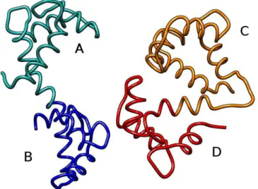
We evaluated our algorithm with respect to accuracy and speed. In order to test the effectiveness of our approach to detect multiple regions of interest, we considered two proteins (PDB IDs 4clna and 2bbma). These proteins are each composed of two similar domains - named A and B (resp. C and D) for the first (resp. second) protein, separated by a flexible bridge (see Fig. 6). The corresponding alignment graph contains 21904 vertices and 40762390 edges (17% of the total number of possible edges).

Figure 6: These two proteins are both composed of two similar domains -named A and B for 4clna (left), and C and D for 2bbma (right). These domains are separated by a a flexible bridge.

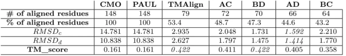
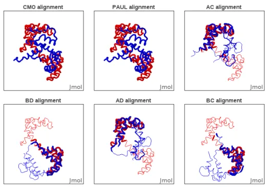
Existing approaches for global protein structure comparison, such as PAUL [31] and ones based on contact map overlap (CMO) [1] tend to match both proteins integrally, yielding larger alignments but poorer RMSD scores. TM_align [33], the reference tool for protein comparison, only matches do-main A onto dodo-main C. The four top results of our tool correspond to all

four possible combinations of domain matching, (see Fig. 7). Our tool was run using 12 cores of an Intel(R) Xeon(R) CPU E5645 @ 2.40GHz and the distance threshold τ was fixed to 3 Ångströms in the alignment graph. Scores corresponding to these alignments are displayed in Table 1.

CMO PAUL TMAlign AC BD AD BC # of aligned residues 148 148 79 72 70 66 64

% of aligned residues 100 100 53.4 48.7 47.3 44.6 43.2 RM SDc 14.781 14.781 2.935 2.048 1.731 1.592 2.210 RM SDd 10.838 10.838 2.627 1.797 1.475 1.414 1.770

TM_score 0.161 0.161 0.422 0.411 0.422 0.405 0.358

Table 1: Details of the alignments returned by other tools - columns 2 through 4 - and our method - columns 5 through 8. Best scores are in italics.

In order to test the efficiency of our coarse-grain parallel implementation, we compare run times obtained with various numbers of threads on a single instance. The input alignment graph for this instance contains 4378 vertices and 525547 edges.3 _{Computations were run using a varying number of cores}

of an Intel(R) Xeon(R) CPU E5-2670 0 @ 2.60GHz. Table 2 shows run times and speedups with respect to the number of CPU cores. Run times displayed in this table are averages out of 100 runs. The table also indicates the standard deviation of each set of 100 runs.

Using more threads for computations provides substantial speedups, but also induces different and unpredictable explorations paths of the search space of the alignment graph. Since finding the optimal set of solutions allows us to prune the search space, the order in which seeds of the graph are considered has an impact on the overall performance of the algorithm. With a single thread, the exploration path of the graph is fixed and run times are homogeneous: the standard deviation with a single thread is 0.9% of the average run time. With more than one thread, the exploration path potentially changes at each run and impacts the total run time. This is par-ticularly true for 2 and 4 threads with standard deviations of respectively 7.6% and 8.4% of the average run time. Further increasing the number of threads reduces the unpredictability by increasing the odds of finding optimal solutions early. This behavior is similar to that exhibited in parallel branch and bound algorithms [15].

3

In order to be able to evaluate more accurately the impact of the number of the threads on the computation time, we have chosen a larger instance than the one used for the same experiment in the conference version of this paper [3].

Figure 7: Visualizations of the results for the comparison of proteins 4clna and 2bbma returned by CMO, PAUL and the four top alignments of our approach.

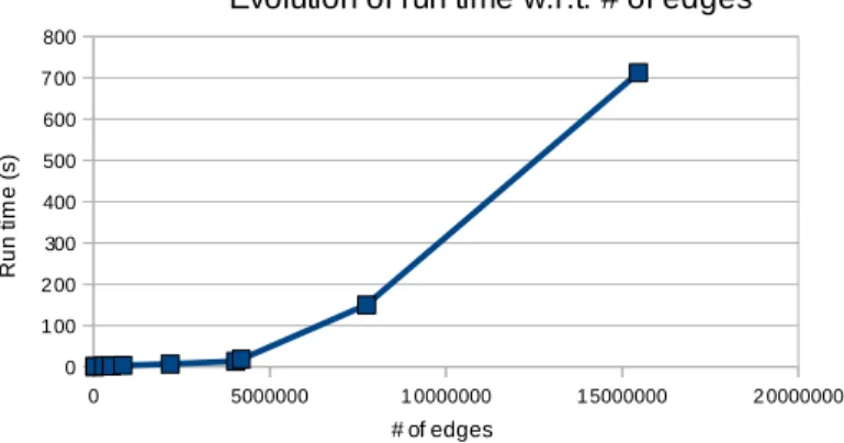
Fig. 8 shows run times for graphs with a varying number of edges and the same number of vertices - 21904. Computations were run using 12 cores of an Intel(R) Xeon(R) CPU E5645 @ 2.40GHz. Input alignment graphs were all generated from the same two proteins and different parameters to allow a varying number of edges. The diagram shows dependence of the run time on the number of edges consistent with the theoretical O(|E|2/3_{), where the}

dependence on |V | is absorbed into the big O factor.

6

Conclusion and perspectives

In this paper, we introduce a novel approach to find similarities between protein structures. Resulting alignments are guaranteed to score well for both

RM SDd and RMSDc, while remaining polynomial. This approach takes

advantage of internal distance similarities, described in an alignment graph, to narrow down the search for an optimal transformation to superimpose two

# of cores 1 2 4 6 8 10 12 14 16

Run time (ms) 49744 25873 14269 10315 8555 7425 6668 6189 5679

Stand. deviation (ms) 458 1969 1192 604 401 284 257 197 193

Stand. deviation (%) 0.9 7.6 8.4 5.9 4.7 3.8 3.9 3.2 3.4

Speedup 1 1.9 3.5 4.8 5.8 6.7 7.5 8.0 8.8

Table 2: Average run times, standard deviation and speedups for varying # of cores. 0 5000000 1 0000000 1 5000000 2 0000000 0 1 00 2 00 300 400 500 600 7 00 800

Evolution of run time w.r.t. # of edges

# of edges R u n t im e ( s )

Figure 8: Evolution of run times with respect to # of edges in an alignment graph of 21904 vertices.

substructures of the proteins.

We consider two main possible directions for extending the results re-ported here: i) improving the performance (accelerating the solver); ii) di-versifying the application area.

6.1

Performance improvement

Though not implemented, an even higher level of parallelism could be consid-ered when graph splitting is performed. Computations for each subgraph are also independent and could therefore be run in parallel. Since a multicore parallelism implementation is already provided, a cluster level parallelism could be implemented. Each subgraph would be sent to a single cluster node using for example using an MPI approach (for Message Passing Inter-face [6]). However, load balancing would be a challenging task due to the limited number of subgraphs that can be generated without a prohibitive loss of accuracy and the difference in terms of numbers of vertices of these subgraphs. Moreover, the total amount of computations would increase if

subgraphs were treated in parallel, since the optimal lower bound found in one subgraph could not be used to solve other subgraphs. This issue would also be similar to that observed in parallel branch and bound algorithms and first described in [15].

The structure of this algorithm as well as the required operations make it suitable for a GPU implementation, which could speed up the compu-tations. A bit-vector implementation for set intersection operations allows regular data access patterns. These access patterns make set intersection operations more cache-friendly and could thus be efficiently mapped to the GPU paradigm. Moreover, GPUs provide all the necessary bit-level instruc-tions such as population cound and bit scanning. Seed listing and result ranking operations are however too irregular to be efficiently computed on a GPU; therefore, seeds could be listed by the CPU and sent to the GPU for extension and filtering operations. Results could then be transferred back to the CPU for ranking operations.

6.2

Diversifying the applications

Detection of structural repeats. A big advantage of the approach is

its capacity to find multiple/alternative alignments with good RMSDc and

RM SDd property. This allows a deeper analysis of protein structures. One

promising perspective is the investigation of repeats inside a protein struc-ture. Structural repeats are common in protein structures [22, 23]. However, they are currently unsatisfactorily studied because of the lack of suitable al-gorithms. Preliminary results show that our approach returns the repetitions in several reliable alignments, so further investigations are in progress.

Combining local alignments into global ones. The idea here to

fur-ther analyze the returned multiple local non-overlapping alignments and to combine them in a new global alignment. Such an approach allows to intro-duce flexibility and non-sequentiality in protein structure alignments. Similar methods already exist such as LGA [32] or FlexSnap [2, 14, 24] and we are currently testing our approach on the corresponding datasets.

Acknowledgment

We are grateful to Noël Malod-Dognin and Frédéric Cazals for motivating discussions in the initial stage of this study.

References

[1] Rumen Andonov, Noël Malod-Dognin, and Nicola Yanev. Maximum contact map overlap revisited. Journal of Computational Biology,

18(1):27–41, 2011.

[2] Christoph Berbalk, Christine S. Schwaiger, and Peter Lackner. Accuracy analysis of multiple structure alignments. Protein Science, 18(10):2027– 2035, 2009.

[3] Guillaume Chapuis, Mathilde Le Boudic-Jamin, Rumen Andonov, Hristo Djidjev, and Dominique Lavenier. Parallel seed-based approach to protein structure similarity detection. In Roman Wyrzykowski, Jack Dongarra, Konrad Karczewski, and Jerzy Wasniewski, editors, PPAM

(2), volume 8385 of Lecture Notes in Computer Science, pages 278–287.

Springer, 2013.

[4] Leonardo Dagum and Ramesh Menon. OpenMP: an industry standard API for shared-memory programming. Computational Science &

Engi-neering, IEEE, 5(1):46–55, 1998.

[5] Jean-Francois Gibrat, Thomas Madej, and Stephen H Bryant. Surpris-ing similarities in structure comparison. Current opinion in structural

biology, 6(3):377–385, 1996.

[6] William Gropp, Ewing L Lusk, and Anthony Skjellum. Using

MPI-: Portable Parallel Programming with the Message Passing Interface,

volume 1. MIT press, 1999.

[7] L Holm and C Sander. Protein structure comparison by alignment of distance matrices. J Mol Biol, 233(1):123–138, 1993.

[8] L Holm and C Sander. Searching protein structure databases has come of age. Proteins, 19(3):165–173, 1994.

[9] George Karypis and Vipin Kumar. A fast and high quality multilevel scheme for partitioning irregular graphs. SIAM Journal on scientific

Computing, 20(1):359–392, 1998.

[10] Patrice Koehl. Protein structure similarities. Current Opinion in

Struc-tural Biology, 11(3):348 – 353, 2001.

[11] Rachel Kolodny, Patrice Koehl, and Michael Levitt. Comprehensive evaluation of protein structure alignment methods: scoring by geometric measures. Journal of molecular biology, 346(4):1173–1188, 2005.

[12] Rachel Kolodny and Nathan Linial. Approximate protein structural alignment in polynomial time. Proceedings of the National Academy of

Sciences of the United States of America, 101(33):12201–12206, 2004.

[13] Janez Konc and Dušanka Janežič. ProBiS algorithm for detection of structurally similar protein binding sites by local structural alignment.

Bioinformatics, 26(9):1160–1168, 2010.

[14] Peter Lackner, Walter A. Koppensteiner, Manfred J. Sippl, and Fran-cisco S. Domingues. ProSup: a refined tool for protein structure align-ment. Protein Eng., 13(11):745–752, November 2000.

[15] Ten-Hwang Lai and Sartaj Sahni. Anomalies in parallel branch-and-bound algorithms. Communications of the ACM, 27(6):594–602, 1984. [16] R H Lathrop. The protein threading problem with sequence amino acid

interaction preferences is NP-complete. Protein Eng, 7(9):1059–1068, 1994.

[17] Pu Liu, Dimitris K Agrafiotis, and Douglas L Theobald. Fast determina-tion of the optimal rotadetermina-tional matrix for macromolecular superposidetermina-tions.

Journal of computational chemistry, 31(7):1561–1563, 2010.

[18] Wei Liu, Anuj Srivastava, and Jinfeng Zhang. A mathematical framework for protein structure comparison. PLoS Comput Biol,

7(2):e1001075, 02 2011.

[19] Noël Malod-Dognin, Rumen Andonov, and Nicola Yanev. Maximum cliques in protein structure comparison. In Paola Festa, editor,

Exper-imental Algorithms, volume 6049 of LNCS, pages 106–117. Springer–

[20] Noël Malod-Dognin and Natasa Przulj. Gr-align: fast and flexible align-ment of protein 3d structures using graphlet degree similarity.

Bioinfor-matics (Oxford, England), Feb 2014.

[21] Shintaro Minami, Kengo Sawada, and George Chikenji. Mican : a pro-tein structure alignment algorithm that can handle multiple-chains, in-verse alignments, calpha only models, alternative alignments, and

non-sequential alignments. BMC Bioinformatics, 14(1):1–22, 2013.

[22] Kevin B Murray, William R Taylor, and Janet M Thornton. Toward the detection and validation of repeats in protein structure. Proteins, 57(2):365–80, November 2004.

[23] R Gonzalo Parra, Rocío Espada, Ignacio E Sánchez, Manfred J Sippl, and Diego U Ferreiro. Detecting repetitions and periodicities in proteins by tiling the structural space. The journal of physical chemistry. B, 117(42):12887–97, October 2013.

[24] Saeed Salem, Mohammed J Zaki, and Chris Bystroff. FlexSnap: flexible non-sequential protein structure alignment. Algorithms for molecular

biology : AMB, 5:12, 2010.

[25] Thomas Schank and Dorothea Wagner. Finding, counting and listing all triangles in large graphs, an experimental study. In Experimental and

Efficient Algorithms, pages 606–609. Springer, 2005.

[26] Stefan Schmitt, Daniel Kuhn, Gerhard Klebe, et al. A new method to detect related function among proteins independent of sequence and fold homology. Journal of molecular biology, 323(2):387–406, 2002.

[27] I N Shindyalov and P E Bourne. Protein structure alignment by in-cremental combinatorial extension (ce) of the optimal path. Protein

Engineering, 11(9):739–747, 1998.

[28] Dawn M. Strickland, Earl Barnes, and Joel S. Sokol. Optimal protein structure alignment using maximum cliques. Oper. Res., 53:389–402, 2005.

[29] S. Subbiah, D.V. Laurents, and M. Levitt. Structural similarity of dna-binding domains of bacteriophage repressors and the globin core.

[30] Inken Wohlers, Rumen Andonov, and Gunnar W Klau. DALIX: Op-timal DALI protein structure alignment. IEEE/ACM Transactions on

Computational Biology and Bioinformatics (TCBB), 10(1):26–36, 2013.

[31] Inken Wohlers, Lars Petzold, Francisco Domingues, and Gunnar Klau. PAUL: Protein structural alignment using integer linear programming and lagrangian relaxation. BMC Bioinformatics, 10(Suppl 13):P2, 2009. [32] Adam Zemla. LGA: a method for finding 3D similarities in protein

structures. Nucleic Acids Research, 31(13):3370–3374, July 2003. [33] Y. Zhang and J. Skolnick. TM-align: a protein structure alignment

algorithm based on the TM-score. Nucleic Acids Res, 33(7):2302–2309, 2005.

[34] Yang Zhang and Jeffrey Skolnick. Scoring function for automated as-sessment of protein structure template quality. Proteins: Structure,