On Financial Markets Incompleteness, Price Stickiness, and Welfare in a Monetary Union

Auray: Université de Lille 3, GREMARS (EA 2459) and CIRPÉE, Maison de la Recherche, Domaine Universitaire du Pont de Bois, BP 149, 59653 Villeneuve d’Ascq cedex, France

stephane.auray@univ-lille3.fr

Eyquem: CREM, Université de Rennes 1, Faculté des Sciences Économiques, 7 place Hoche, 35065 Rennes Cedex

aurelien.eyquem@univ-rennes1.fr

We would like to thank Hafedh Bouakez, Daniel Browne, Arianna Degan, Gordon Fisher, Paul Gomme and Tatyana Koreshkova for helpful comments. This draft was completed while Auray was visiting the department of economics at Concordia University, Montreal. He is grateful for their kind hospitality. The traditional disclaimer applies.

Cahier de recherche/Working Paper 07-48

On Financial Markets Incompleteness, Price Stickiness, and Welfare

in a Monetary Union

Stéphane Auray

Aurélien Eyquem

Décembre/December 2007

(First version : March 2007)

Abstract:

In this paper, we measure the welfare costs/gains associated with financial market

incompleteness in a monetary union. To do this, we build on a two-country model of a

monetary union with sticky prices subject to asymmetric productivity shocks. For

most plausible values of price stickiness, we show that asymmetric shocks under

incomplete financial markets give rise to a lower volatility of national inflation rates,

which proves welfare improving with respect to the situation of complete financial

markets. The corresponding welfare gains are equivalent to an average increase of

1.8% of permanent consumption.

Keywords: Monetary union, asymmetric shocks, price stickiness, financial markets

incompleteness, welfare

1

Introduction

Financial markets integration is traditionally considered of great importance for the smooth functioning of the European Monetary Union as it constitutes an insurance mechanism fostering symmetric adjustment to asymmetric shocks. As a matter of fact, the costs of incompleteness in financial markets, approximating imperfect financial integration, have been widely documented (see, for instance, Cole and Obstfeld [1991] and Kim, Kim and Levin [2003a]). More recently, using a two-country model subject to asymmetric productivity shocks, Benigno [2007] shows that imperfect risk-sharing and the corresponding path of the real exchange rate generate welfare costs under flexible prices allocations.1 Means to reduce these costs have also been explored in the literature. For example, Cole and Obstfeld [1991] show that these types of costs might be reduced by achieving a deeper trade integration, since incomplete financial market allocations may replicate the complete asset markets allocations under specific hypotheses. In this paper, we argue that the dynamics of inflation under alternative financial structures is likely to impact the costs of financial markets incompleteness, by affecting real exchange rate dynamics and the pattern of external adjustment.

Focusing on the euro area, recent empirical and theoretical evidence suggest that the common monetary policy has been successful at keeping aggregate inflation low. However, they also point out the impossibility for policymakers to address the consequences of asymmetric shocks on national inflation rates. These sets of evidence lead us to raise the following question: what are the welfare costs/gains associated with incomplete financial markets in a monetary union with idiosyncratic productivity shocks and sticky prices? To address this question, we follow Benigno [2007] and consider a two-country model of a monetary union with sticky prices subject to idiosyncratic productivity shocks. We model financial markets either as a continuum of state-contingent assets, or as a single bond market. Under complete financial markets, each agent has the same wealth and the Backus-Smith risk-sharing condition holds. Under incomplete financial markets, agents trade composite bonds and use financial markets to smooth their adjustment to asymmetric shocks, thereby restoring the external adjustment channel of the current account. However, since this solution generates a unit root on net foreign assets dynamics, we follow Schmitt-Grohe and Uribe [2003] and assume the existence of financial intermediaries levying portfolio management quadratic costs, depending on the level of bonds traded.

We differ from Benigno [2007] by allowing sticky prices to generate additional inefficiencies. We show that the optimal targeting rules implied by the optimal policy stabilize the aggregate inflation rate and close the aggregate consumption gap.2 However, monetary instrument rules that the common central bank may actually use to stabilize the economy, i.e. using a single interest rate, prevent the stabilization of national inflation rates, which generates additional welfare losses with respect to the optimal policy. These losses are crucial in generating our results.

Based on this framework, we evaluate the welfare costs that a monetary union may endure when financial market are complete vs incomplete under simple interest rate rules stabilizing the aggregate inflation rate and consumption gap. We more specifically highlight the key role of the assumption of price stickiness in determining the Pareto–dominant situation. When prices are flexible, incomplete financial markets imply imperfect risk–sharing that turns to welfare losses. These results are consistent with the ones of Kim et al. [2003a]. This case also corresponds to the situation where independent national monetary policies stabilize national inflation rates. Under such a policy, the volatility of inflation rates and their related welfare losses are equal to zero. Our results thus comfort those of Benigno [2007]. In line with Cole and Obstfeld [1991], we also find that a better integration of goods markets, approximated by an increase of the openness parameter or an increase of the elasticity of substitution between domestic and foreign goods, lowers the welfare losses of imperfect financial integration. When prices are sticky, we show that financial markets incompleteness implies a lower volatility of national inflation rates, thereby generating welfare gains with respect to the situation of complete financial markets. Under incomplete financial markets, agents may use financial markets and the channel of the current account to adjust externally and to smooth their consumption profiles in time, thus lowering the pressure on the terms of trade. As a consequence, the degree of volatility of national inflation rates required to adjust to asymmetric shocks is lower. This mechanism leads to significant welfare gains that more than compensate the welfare losses due to imperfect risk–sharing.

The paper is structured as follows. Section 2 presents the model. Section 3 describes the dynamics of the model and the authorities’ loss function. Section 4 determines the optimal (Ramsey) policy. Section 5 analyzes the dynamics of the model after an asymmetric productivity

2_{In the model, we assume that governments offset first–order distortions, thereby restoring the Pareto–efficiency}

of the steady state. This assumption also avoids that optimal monetary policy targets a non–zero aggregate inflation rate.

shock. Section 6 presents the welfare costs of complete versus incomplete financial markets and proceed to some robustness experiments. Conclusions are summarized in Section 7.

2

A two–country model

The model describes a two–country monetary union with a common central bank that controls the nominal interest rate. Each country is populated by a continuum of households of infinite life, an infinite number of firms that are specialized in the production of differentiated goods and a government. Goods markets are characterized by a home bias in consumption bundles and Calvo–staggered adjustment of prices.

2.1 Households and financial markets

In each country the representative household j ∈ [0, 1] of country i ∈ {h, f } maximizes a welfare index, ω_ti(j) = ∞ X t=0 βtE0 ½ C_ti(j)1−ρ 1 − ρ − N_ti(j)1+ψ 1 + ψ ¾ , (1)

subject to the budget constraint,3

B_t+1i (j) − R_tBi_t(j) = W_tiN_ti(j) + Π_ti(j) − P_tiC_ti(j) − P_i,tAC_ti(j) − T_ti(j), (2) and the transversality condition, lim_{T →∞}ΠT

τ =tR−1τ Et © Bi T +1(j) ª = 0. In (1), the parameter

β = (1 + δ)−1 _{is the subjective discount factor, C}i

t(j) is the consumption bundle chosen by

the representative agent, Ni

t(j) is its competitive labor supply, ρ is the degree of consumption

risk–aversion and ψ−1 _{is the elasticity of labor supply. In (2),W}i

t is the nominal wage in country

i for period t, Πi

t(j) =

R₁

0 Πit(k, j)dk is the profit paid by national firms to the representative

national agent j. Bi

t(j) corresponds to the holding of the composite one–period nominal bond at

the end of period (t − 1) which pays a gross nominal rate of interest R_tbetween periods (t − 1) and t, Ti

t(j) is a lump-sum tax paid by household j to the national government of country i.

Finally, Pi

t is the consumer price index in country i in period t, Pi,t is the producer price index in

country i in period t and ACi

t(j) is a portfolio adjustment cost paid in units of domestic goods.

In the case detailed above, the financial market of the monetary union is incomplete and households trade a one–period composite financial asset. Buying (resp. selling) bonds affects

3_{The model features no money holdings, since money is endogenously supplied depending on the level of}

negatively (resp. positively) the individualized interest rate, so that: (i) agents have a strong incentive to return to their initial position in the long run; and (ii) agents belonging to a creditor country face lower nominal interest rates than agents in the debtor country. As underlined by Schmitt-Grohe and Uribe [2003], this assumption is a convenient way to balance the current account in the long run between union members while preserving its short–run dynamics. We impose a standard quadratic form for portfolio adjustment costs,

AC_ti(j) = χ 2 £

B_t+1i (j) − Bi(j)¤2.

where Bi_{(j) is the steady state level of financial assets hold by agent j in country i. Portfolio}

adjustment costs affect the Euler condition since,

βI_t+1i Et ½ Pi tCti(j)ρ Pi t+1Ct+1i (j)ρ ¾ = 1, (3) with, Ii t+1(j) = Rt+1 £ 1 + χPi,t(Bt+1i (j) − Bi(j)) ¤₋₁

. The value of χ affects the intertemporal consumption choice in (3): an increase in the cost of bond trading reduces the sensitivity of wealth accumulation to variation in the interest rate, because it becomes more costly to smooth consumption.

In the case of complete markets, agents are supposed to have access to a continuum of Arrow–Debreu securities and portfolio costs vanish (χ = 0 and ACi

t = 0). In such a case,

the Backus–Smith condition holds, implying that each agent’s wealth is the same across the monetary union,

P_thC_th(j)ρ= P_tfC_tf(j)ρ, ∀t.

The labor supply function is standard since it depends on the level of consumption and the real wage,

N_ti(j)ψ = Wti

Pi

tCti(j)ρ .

Following Corsetti [2006], we assume home bias in final consumption bundles. The consump-tion bundle of consumer j living in country i, Ci

t(j), is C_ti(j) = · (1 − αi) 1 µ¡Ci h,t(j) ¢µ−1 µ _{+ α} 1 µ i ¡ C_f,ti (j)¢µ−1µ ¸ µ µ−1 ,

and the companion consumption price index Pi t is, P_ti = h (1 − αi) ¡ P_h,ti ¢1−µ+ αi ¡ P_f,ti ¢1−µ i 1 1−µ ,

where αi∈

£

0,1₂¤is the home bias, which also measures the openness of the final goods market in country i, and µ is the elasticity of substitution between domestic and foreign goods.

Consumption subindexes are,

C_h,ti (j) = ·Z ₁ 0 C_h,ti (k, j)θ−1θ dk ¸ θ θ−1 , and C_f,ti (j) = ·Z ₁ 0 C_f,ti (k, j)θ−1θ dk ¸ θ θ−1 . Ci

h,t(k, j) (resp. Cf,ti (k, j)) is the consumption of a typical final good k of home (resp. foreign)

country by the representative consumer j of country i and θ > µ is the elasticity of substitution between national varieties of final goods. We assume that firms do not discriminate the market they address and that their retail prices are identical in both countries. The corresponding prices of domestic and foreign goods in country i are, Pi

h,t = Ph,t = [ R₁ 0 Ph,t(k)1−θdk] 1 1−θ and Pi f,t= Pf,t = [ R₁ 0 Pf,t(k)1−θdk] 1 1−θ, respectively.

Accordingly, optimal variety demands are,

C_h,ti (k, j) = (1 − αi) · Ph,t Pi t ¸_−µ· Ph,t(k) P_h,t ¸_−θ C_ti(j), C_f,ti (k, j) = αi · Pf,t Pi t ¸_−µ· Pf,t(k) P_f,t ¸_−θ C_ti(j).

Since portfolio costs are paid in units of goods, i.e. AC_ti(j) = [R₀1AC_ti(k, j)θ−1θ dk] θ

θ−1, they

imply variety demands, defined as ACi

t(k, j) = h Ph,t(k) Ph,t i_−θ ACi t(j).

Finally, we define the terms of trade as,

St= P_Pf,t

h,t .

2.2 Firms

Firms produce k varieties in country i ∈ {h, f } using national labor according to a standard technology,

Y_ti(k) = Ai_tLi_t(k), with Ai_t+1= (1 − ρa) Ai+ ρaAit+ ξt+1i ,

where ξi

t+1 is an i.i.d innovation.

Following Calvo [1983], we assume that in economy i ∈ {h, f }, a fraction¡1 − ηi¢of randomly selected firms is allowed to set new prices each period. Firms set prices higher in comparison of the typical mark-up pricing, depending on the expected period during which they will be unable to reset. The corresponding optimal price is,

P_i,t∗(k) = θ (θ − 1) (1 − τ ) ∞ X v=0 ¡ ηiβ¢vEt ½ Yi t+ν(k) Pi t+νCt+νi (j)ρ W_ti/Ai_t ¾ ∞ X v=0 ¡ ηiβ¢vEt ½ Yi t+ν(k) Pi t+νCt+νi (j)ρ ¾ .

In this expression, τ is a subsidy that compensates the distorting effects of monopolistic competition in the economy.4 _Yi

t(k) is the aggregate demand facing firm k on the final goods

market. Aggregating among final firms and assuming behavioral symmetry of Calvo producers, the average price of final goods in nation i ∈ {h, f } is,

Pi,t= h¡ 1 − ηi¢P_i,t∗(k)1−θ+ ηiP_i,t−11−θ i 1 1−θ . 2.3 Governments

Fiscal policy is aimed at closing first order distortions related to the monopolistic structure of final goods markets. Governments finance the corresponding subsidy made to firms through a lump-sum tax on households. Their budget constraint is,

Z ₁ 0 T_ti(j)dj = −τ Z ₁ 0 Pi,t(k)Yti(k)dk. 2.4 General equilibrium

For any sequence of productivity shocks n

Ah

t, Aft

o_∞

t=0, an equilibrium is a sequence of quantity{Qt} ∞ t=0 where Qt= n Yh t , Ytf, Cth, Ctf, Nth, Ntf, Bth, Btf, ACth, ACtf o_∞

t=0that satisfies households and firms

optimality conditions for a given set of prices {P_t}∞_t=0= n

Wh

t, Wtf, Pth, Ptf, Ph,t, Pf,tf , Ph,t∗ (k), Pf,t∗ (k)

o_∞

t=0

in a way that is compatible with the clearing of markets described below. Defining aggregate supply bundles as Yi

t = hR₁ 0 Yti(k) θ−1 θ dk i θ θ−1

and assuming α_h = α and

αf = 1 − α, final goods markets clear according to, Y_th = (1 − α) · Ph,t Ph t ¸_−µ C_th+ α " Ph,t P_tf #_−µ C_tf + AC_th, Y_tf = (1 − α) " P_f,t P_tf #_−µ C_tf+ α · P_f,t Ph t ¸_−µ C_th+ AC_tf.

Labor is immobile, so that Ni

t =

R₁

0 Nti(j)dj =

R₁

0 Lit(k)dk, and the aggregate production

function of country i ∈ {h, f } is Yi

tDPi,t = AitNti, where DPi,t =

R₁ 0 h Pi,t(k) Pi,t i_−θ dk ≥ 1 is the

dispersion of production prices in country i.

The international financial market clearing condition is, Z ₁ 0 B_th(j)dj + Z ₁ 0 B_tf(j)dj = 0.

4_{Monopolistic competition distorts the first-best allocation through mark-up pricing and a lower output. As}

shown by Benigno and Woodford [2005], an optimal subsidy policy restores the optimal perfectly competitive allocation.

Finally, consolidating households, governments and firms resources constraints, the dynamics of net foreign assets in country h is given by

B_t+1h − RtBth= Ph,tYth− PthCth. (4)

3

A linear-quadratic framework

We solve the model applying standard linearization methods. We first define the optimal mon-etary policy as the minimization of a welfare loss function constrained by the model. This approach usually requires that the model is solved with a second order approximation, to avoid spurious welfare reversals documented by Kim, Kim and Levin [2003b]. However, Benigno and Woodford [2006] have shown that the solution of the optimal policy problem can be set in the convenient linear-quadratic form while remaining valid when the second order approximation of the welfare–based loss function yields a purely quadratic function, which is the case in our framework.

3.1 Steady state

We solve the model in logdeviation with respect to the symmetric steady state. In the symmetric steady state Ai _{= A = 1 and B}i _{= B = 0. Symmetry imposes P}

h = Pf = Ph = Pf = Pi∗(k)

= P , implying, Wi

Pi = W_P =

(θ−1)(1−τ )

θ A. The compensation of first order distortions requires

that the government sets τ = (1 − θ)−1 ≤ 0, implying W_P = A. Portfolio costs are zero so that

I = R = β−1_{. Price indexes are such that DP = 1, final goods markets give C = Y , and the}

production function is Y = AN . Combining these relations with the leisure arbitrage, we get,

Y = A1+ψψ+ρ. For tractability, we simply assume A = 1, implying Y = C = N = W

P = 1. Since

the model features no money holding, the price level is defined arbitrarily to P = 1.

3.2 The model in deviation from the natural equilibrium

The natural equilibrium, corresponding to the flexible price equilibrium with complete financial markets, is considered as the benchmark for the definition of the optimal policy. We thus express the linear dynamics of the model in deviation from the natural equilibrium. Applying the standard linearization procedure, we consider xi

t as the logdeviation of Xti, ∀t for i ∈ {h, f }

from the steady state. Defining ext as the natural equilibrium dynamics of xt, we finally define

3.2.1 The case of complete financial markets

Under complete financial markets, the model expressed in deviation from the natural equilibrium is given by b nr_t = −$αbst, (5) ρEt © b cu_t+1− bcu_tª = δ 1 + δbrt+1− Et © πu_t+1ª, (6) ρEt © b cr_t+1− bcr_tª = − (1 − 2α) Et © πr_t+1ª, (7) πh,t = βEt{πh,t+1} + kh · (ρ + ψ) bcu_t − ψbnr_t +1 2bst ¸ , (8) πf,t = βEt{πf,t+1} + kf · (ρ + ψ) bcu_t + ψbnr_t−1 2sbt ¸ , (9) b st− bst−1 = πf,t− πh,t+_{1 + 2ψ$}2 (1 + ψ) αa r t− 2 (1 + ψ) 1 + 2ψ$αa r t−1, (10) where $_α= (1−2α)2+4ρµα(1−α)_2ρ and ki ₌ (1−ηiβ)(1−ηi) ηi . In these expressions, exu_t = 1₂(exh_t + exf_t ) is

the average value of Xt in the monetary union and exrt = 12(exft− exht) its relative value. Eq. (5) is

the contraction of the relative expression of the final goods market equilibria (for the right-hand side element) and the relative production functions (for the left-hand side element). Eqs. (6) and (7) summarize the relative and union-wide expressions of Euler equations. Eqs. (8) and (9) are the expressions for modified Phillips curves, obtained by expressing marginal cost in terms of variables in deviation from the natural equilibrium.

3.2.2 The case of incomplete financial markets

We now expose the dynamic equilibrium under incomplete financial markets. Since B = 0, we define the loglinear expression of Bi

t as bit = B

i t/C

Pi

t . The model in deviation from the natural

equilibrium under incomplete financial markets is, b nr_t = (1 − 2α) bcr_t− 2µα (1 − α) bs_t, (11) ρE_t©bcu_t+1− bcu_tª = δ 1 + δbrt+1− Et © π_t+1u ª, (12) ρE_t©bcr_t+1− bcr_tª = χbbh_t+1− (1 − 2α) E_t©πr_t+1ª, (13) π_h,t = βE_t{π_h,t+1} + kh[(ρ + ψ) bcu_t − ψbnr_t− ρbcr_t + αbs_t] , (14) π_f,t = βE_t{π_f,t+1} + kf[(ρ + ψ) bcu_t + ψbnr_t + ρbcr_t− αbs_t] , (15) b s_t− bs_t−1 = π_f,t− π_h,t+ 2 (1 + ψ) 1 + 2ψ$α ar_t − 2 (1 + ψ) 1 + 2ψ$α ar_t−1, (16) bbh t+1− bbht = δbbht + α [2µ (1 − α) − 1] bst+ 2αbcrt. (17)

The equations are slightly modified with respect to the case of complete financial markets. Since the Backus-Smith condition does not hold anymore, Eq.(11) indicates that the equilibrium of the final goods markets depends both on relative consumption and on the terms of trade. Eq.(12) is unchanged. Eq.(13) is the contraction of Euler equations and shows how that the Backus-Smith condition is broken, since χbbh_t+1 is the gap between relative consumptions and the terms of trade. Using the current account bbh

t+1 to adjust externally clearly increases the

distance from perfect international risk-sharing. Eqs. (14) and (15) are the expressions for modified Phillips curves when relative consumptions and the terms of trade are not tied by the Backus-Smith condition. Eq.(16) is unchanged. Finally, Eq.(17) describes the dynamics of net foreign assets where α [2µ (1 − α) − 1] bst+ 2αbcrt is the trade balance.

3.3 The authorities loss function

To determine the optimal policy and to rank alternative situations, we adopt a welfare measure based on the aggregate utility function,

ωT = 1₂ Z ₁ 0 ωh_T(j)dj +1 2 Z ₁ 0 ω_Tf(j)dj, where, after using symmetry among agents,

ωi_T(j) = ω_Ti = T X t=0 βtE₀ ( ¡ Ci t ¢_1−ρ (1 − ρ) − ¡ Ni t ¢_1+ψ (1 + ψ) ) .

The welfare measure is computed using second–order approximations of ωT and equilibrium

conditions, and expressed as a quadratic function of endogenous variables in deviation from their natural equilibrium paths,

ωT = − C1−ρ 2 T X t=0 βtE0{ θ 2khπh,t2 + θ 2kfπf,t2 + (ρ + ψ) [bcut] 2 + µα (1 − α) [bst]2+ ρ [bcrt]2+ ψ [bnrt]2} + t.i.p + O ¡° °ξ3°_°¢_{. (18)} The welfare measure (18) admits standard arguments, such as national inflation rates and the aggregate consumption gap. However, the welfare measure also penalizes regional asymmetries, since deviations of terms of trade, of relative consumption and of relative effort are costly.

4

Optimal policy under complete financial markets

In this section, we compute the optimal plan under complete financial markets. It is defined as the minimization of the welfare loss function (18) subject to the linear dynamic system (5)-(10).

Assuming that the social planner can commit for an infinity of periods and adopting Wood-ford’s (2003) timeless perspective, the optimal policy is obtained by minimizing the following Lagrangian, L = T X t=0 βtEt{_2kθ_hπ2h,t+ θ 2kfπf,t2 + (ρ + ψ) [bcut]2+ µα (1 − α) [bst]2+ ρ [bcrt]2+ ψ [bnrt]2 + 2Λ1,t · πh,t− βEt{πh,t+1} − kh · (ρ + ψ) bcu_t − ψbnr_t+1 2bst ¸¸ + 2Λ2,t · π_f,t− βEt{πf,t+1} − kf · (ρ + ψ) bcu_t + ψbnr_t −1 2bst ¸¸ + 2Λ3,t · b st− bst−1− πf,t+ πh,t− 2 (1 + ψ) 1 + 2ψ$αa r t+ 2 (1 + ψ) 1 + 2ψ$αa r t−1 ¸ }.

After some algebra, first order conditions collapse to the following optimal targeting rules,

θ 2(πh,t+ πf,t) = − (1 − κ) ¡ b cu_t − bcu_t−1¢− Λ3,t ³ kh− kf ´ , θ 2(πf,t− πh,t) = − ¡ b nr_t − bnr_t−1¢+ Λ3,t ³ kh+ kf ´ , (Λ3,t−1− βΛ3,t) = −$αsbt−1− αbnrt−1, bcr_t = −(1 − 2α) 2ρ bst, augmented with the following constraints,

π_h,t = βEt{πh,t+1} + kh · (ρ + ψ) bcu_t − ψbnr_t+1 2bst ¸ , π_f,t = βE_t{π_f,t+1} + kf · (ρ + ψ) bcu_t + ψbnr_t −1 2bst ¸ , b st− bst−1 = πf,t− πh,t+ 2 (1 + ψ) 1 + 2ψ$_αa r t − 2 (1 + ψ) 1 + 2ψ$_αa r t−1.

The corresponding 7 equations - 7 variables recursive system requires that the condition

kh _{= k}f _{= k is verified to have a unique and stable solution.}

In the equilibrium, combining the first optimal targeting rule with the Phillips curves implies that the aggregate inflation rate is fully stabilized (πu

t = 0) and that the aggregate consumption

gap is closed (byu

t = 0). This result is quite standard in the literature and implies that the

optimal instrument rule is to equate the nominal interest rate to the natural interest rate. However, the solution of the optimal monetary policy problem also features some motivation for regional stabilization. These goals are clearly beyond the control of the common central bank and the optimal plan as a whole can not be decentralized due the restricted set of available policy instruments.

For that reason, next sections explore the welfare implications of alternative financial struc-tures under monetary policies that the common central bank may actually implement (brt+1= 0).

In the rest of the paper, we refer to these policies as feasible policies. The corresponding wel-fare losses are expressed in terms of their distance to the optimal plan under complete financial markets.

5

Dynamics under feasible monetary policy

In this section, we calibrate the model under both complete and incomplete financial markets. We then analyze the dynamic properties in both cases and highlight the mechanisms behind our results.

5.1 Baseline calibration

We calibrate the deep parameters of the model based on standard values found in the literature. Following Beetsma and Jensen [2005], the intertemporal elasticity of substitution is ρ = 2. The value of ψ refers to Canzoneri, Cumby and Diba [2006] and varies between 5 and 15. For the baseline case, we choose ψ = 5. In the literature, estimates of µ, the elasticity of substitution between domestic and foreign goods, range from 1 to 15. For example, estimates of Harrigan [1993] range from 5 to 12. We set µ = 2 and then check for robustness with other values of this parameter. The elasticity of substitution across varieties determines the average mark-up, which according to Rotemberg and Woodford [1997] is around 16-17% , implying θ = 7. We set the openness parameter to α = 0.25 in the benchmark calibration and, following Faia [2007], we let it vary from 0.25 to 0.4. The parameter controlling nominal rigidities ranges, according to different estimates, from 0.5 to 0.8. Following Canzoneri et al. [2006], we set the baseline value at ηh _{= η}f _{= 0.75. The portfolio cost parameter χ is set to 0.001, corresponding to an}

average annual interest rate premium of 0.405%, in line with Schmitt-Grohe and Uribe [2003] and Benigno [2007]. Other parameters are fairly standard: β = 0.988, ρa= 0.95 and std

¡

ξi

t

¢

= 0.7%.

5.2 Dynamics under complete financial markets

In the case of complete financial markets, the perfect risk-sharing condition holds implying that relative wealth in each country is the same, namely,

bcr_t = −(1 − 2α) 2ρ bst.

The intuition behind our results is that the pattern of external adjustment after an asymmet-ric productivity shock and its internal consequences, as it can be seen through the expressions of New-Keynesian Phillips curves, may significantly affect inflation dynamics, which is the most heavily weighted component of the welfare measure (Eq. 18).

Under complete financial markets, the dynamic system is described by Eqs. (5)-(10) and by b

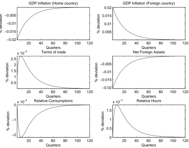
rt+1 = 0, ∀t. Figure 1 plots the IRF of interest variables in the monetary union after a unit

domestic productivity innovation in the case of complete financial markets.

A productivity shock generates a deflation at home and the nominal interest rate drops to stabilize aggregate inflation. This policy translates into a positive demand shock for the foreign country and implies a significant inflation in this country (exactly equal to the domestic deflation). The dynamics of inflation rates generates a positive (resp. negative) wealth effect for home (resp. foreign) agents, allowing them to sustain higher (resp. lower) consumption levels. The corresponding negative relative consumption gap implies a positive terms of trade gap through the Backus-Smith condition. In other words, the terms of trade increase more than in the natural equilibrium to meet the external equilibrium. The global pattern of external adjustment relies entirely on terms of trade and the current account does not play any role.5

5.3 Dynamics under incomplete financial markets

The main difference with last paragraph is the introduction of an additional external adjustment channel through the current account. As a consequence, paths of relative consumption and terms of trade are determined independently. Under incomplete financial markets, the economy evolves according to the system (11)-(17) augmented with the monetary policy brt+1= 0, ∀t.

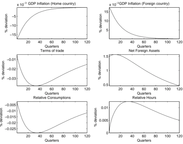
Figure 2 depicts the responses to a unit domestic productivity innovation. Similar to the case of complete financial markets, domestic inflation falls and foreign inflation increases. The adjustment pattern is somewhat different, however. The fall and rise of home and foreign inflation is stronger in the first periods but the absolute cumulated response is lower.6 _{The gap} in relative consumptions is still negative, implying that home agents sustain higher consumption levels thanks to the wealth effect induced by national inflation rates dynamics. Contrary to the

5_{In the simple case of unitary elasticity of substitution between home and foreign goods, complete financial}

markets even imply a constant zero net foreign assets position (see Lane and Milesi-Ferretti [2001]). Otherwise, net foreign assets are determined after terms of trade dynamics and do not enter in the definition of the dynamic equilibrium.

6_{The cumulated response of inflation is ±0.3867 under incomplete financial markets and ±0.3929 under}

Figure 1: Impulse response functions to a unit productivity innovation under complete financial markets. 20 40 60 80 100 120 −0.02 −0.015 −0.01 −0.005

GDP Inflation (Home country)

Quarters % deviation 20 40 60 80 100 120 0.005 0.01 0.015 0.02

GDP Inflation (Foreign country)

Quarters % deviation 20 40 60 80 100 120 0.5 1 1.5 2 2.5 x 10−3 Terms of trade Quarters % deviation 20 40 60 80 100 120 −0.02 −0.015 −0.01 −0.005

Net Foreign Assets

Quarters % deviation 20 40 60 80 100 120 −2 −1 0x 10 −4 _{Relative Consumptions} Quarters % deviation 20 40 60 80 100 120 0 0.5 1 1.5 x 10−3 Relative Hours Quarters % deviation

Figure 2: Impulse response functions to a unit productivity innovation under incomplete financial markets. 20 40 60 80 100 120 −15 −10 −5

x 10−3GDP Inflation (Home country)

Quarters % deviation 20 40 60 80 100 120 5 10 15

x 10−3GDP Inflation (Foreign country)

Quarters % deviation 20 40 60 80 100 120 −0.03 −0.02 −0.01 Terms of trade Quarters % deviation 20 40 60 80 100 120 0.5 1 1.5

Net Foreign Assets

Quarters % deviation 20 40 60 80 100 120 −0.025 −0.02 −0.015 −0.01 −0.005 Relative Consumptions Quarters % deviation 20 40 60 80 100 120 0 0.005 0.01 Relative Hours Quarters % deviation

case of complete financial markets, the gap in terms of trade is negative. In the case of incomplete financial markets, terms of trade volatility is lower than under complete financial markets and lower than in the natural equilibrium. When shocks are transitory, agents are more prone to use the current account as a device to smooth consumption over time and rely less on terms of trade to adjust externally. Consequently, the shock implies an accumulation of net foreign assets and terms of trade do not increase as much as they would with purely flexible prices, translating into a negative terms of trade gap.

External adjustment to asymmetric shocks relies exclusively on relative prices under complete financial markets and more on quantities under incomplete markets. As a consequence, terms of trade gaps are more volatile under incomplete financial markets but terms of trade variations (s_t − s_t−1 = π_f,t − π_h,t) and national inflation rates (π_f,t and π_h,t) are less volatile. Since the volatility of national inflation rates is the most weighted component of the welfare loss function, incomplete financial markets exhibit welfare enhancing properties that may reverse the traditional welfare costs associated with financial markets incompleteness.

6

Welfare costs/gains

In this section, we measure the welfare costs or gains arising under alternative financial structures in a monetary union subject to asymmetric productivity shocks. We highlight (i) the welfare losses of incomplete financial markets when prices are flexible and (ii) the welfare gains of incomplete financial markets when the degree of price stickiness reaches a certain threshold. In such a case, we show that financial markets incompleteness is associated with a lower volatility of national inflation rates since the external adjustment after asymmetric productivity shocks relies more on quantities and less on terms of trade. For most plausible values of parameters and as long as η is larger than 0.4, we provide evidence that the corresponding welfare gains more than compensate the welfare costs related to imperfect risk-sharing. Finally, we assess the robustness of our results by running a sensitivity analysis.

Welfare gains are expressed in terms of permanent consumption, so that, ΩT = 100 · · 1 − β ρ + ψ ³ ωref_T − ωT ´¸1 2 , where ωref

T is the welfare in the reference situation. In order to decompose our results, the

reference situation will be the optimal plan under complete financial markets and the feasible policy under complete financial markets alternatively.

6.1 Price stickiness and welfare

Welfare losses of alternative financial structures and monetary policies are reported in Table 1. Table 1: Welfare losses.

Flexible prices∗ _{Sticky prices}

Ω_inc/com Ω_com/opt Ω_inc/opt Ω_inc/com

Baseline 0.46 1.12 -1.41 -1.80 ψ = 10 0.33 0.84 -0.90 -1.23 ψ = 15 0.27 0.70 -0.69 -0.98 ρ = 1 0.50 1.11 -1.62 -1.97 ρ = 5 0.37 0.99 -1.09 -1.47 α = 0.35 0.25 0.95 -0.92 -1.32 α = 0.4 0.16 0.90 -0.76 -1.18 α = 0.5 0.00 0.87 -0.53 -1.01 µ = 1 0.83 2.25 -2.91 -3.68 µ = 5 0.20 0.41 -0.46 -0.62 µ = 10 0.10 0.21 -0.19 -0.28 η = 0.7 - 0.79 -1.15 -1.40 η = 0.8 - 1.69 -1.70 -2.40 ρa= 0.9 1.02 3.94 -1.23 -4.12 ρa= 0.99 0.07 0.13 -0.25 -0.28 ∗ for stability reasons, we set η = 0.0001 ' 0

Note: for α = 0.5 under flexible prices, the loss is 0.0001%.

Consistent with other studies (see Kim et al. [2003a]), when prices are flexible, we find that incomplete financial markets imply imperfect risk-sharing, generating welfare losses rising to an average decrease of permanent consumption of about 0.5% (first column of Table 1). Alter-natively, interpreting the situation of flexible prices as a situation where independent national monetary policies stabilize national inflation rates, our results comfort those of Benigno [2007], especially when home bias in consumption vanishes (α = 1₂). We also find that a better inte-gration of goods markets, approximated by an increase of the openness parameter (α) or an increase of the elasticity of substitution (µ), may lower the welfare losses of imperfect financial integration, as documented by Cole and Obstfeld [1991].

When prices are sticky, we highlight the fact that inflation variability is lower under in-complete financial markets. As demonstrated by the analysis of response functions after an asymmetric home productivity shock, incomplete financial markets introduce an additional ex-ternal adjustment channel and restore the role of the current account. Since agents may use this

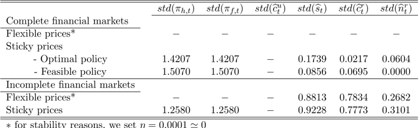
channel to adjust externally, the pressure on terms of trade is lower. As a consequence, national inflation rates are much less volatile for most plausible values of parameters of the model, as depicted in Table 2. The volatility of inflation rates is even lower under incomplete financial markets and feasible monetary policy than in the case of complete financial under the optimal plan.

Table 2: Standard deviations (%) - Baseline calibration.

std(π_h,t) std(π_f,t) std(bcu

t) std(bst) std(bcrt) std(bnrt)

Complete financial markets

Flexible prices* − − − − − −

Sticky prices

- Optimal policy 1.4207 1.4207 − 0.1739 0.0217 0.0604 - Feasible policy 1.5070 1.5070 − 0.0856 0.0695 0.0000 Incomplete financial markets

Flexible prices* − − − 0.8813 0.7834 0.2682

Sticky prices 1.2580 1.2580 − 0.9228 0.7773 0.3101

∗ for stability reasons, we set η = 0.0001 ' 0

In the loss function and for the baseline calibration, weights on inflation are _2kθ ' 40 while

weights on terms of trade gaps in relative consumptions and relative hours are respectively

µα (1 − α) ' 0.37, ρ = 2 and ψ = 5. As a consequence, welfare gains associated with lower

volatility of inflation rates more than compensate for welfare losses related to higher volatility of gaps in terms of trade, relative consumptions or relative hours. The situation of incom-plete financial markets thus Pareto–dominates the situation of comincom-plete financial markets in a monetary union characterized by sticky prices.

The welfare gains reported in the third and fourth column of Table 1 are clearly related to the reduction of the volatility of inflation rates caused by the use of the current account in the external adjustment of the economies. In this case, the distortion related to financial markets incompleteness, which is costly in terms of welfare when prices are flexible, generates a positive externality through a lower volatility of national inflation rates. The situation of incomplete financial markets thus enhances the welfare of about 1.8% in average with respect to the situation of complete financial markets under feasible monetary policy.

6.2 Sensitivity analysis

The sensitivity results may be summarized as follows:

(i): The Frischian elasticity ψ lowers the welfare losses independently of the financial

struc-ture, since fluctuations have less impact on hours worked.

(ii): The risk aversion parameter ρ is one of the most important. Under incomplete financial

markets, an increase of ρ increases agents’ incentives to smooth consumption over time when (unanticipated) transitory shocks arise. By this effect, ρ has a positive impact on welfare gains. However, under complete financial markets, the Backus-Smith condition is binding and implies that, for a given volatility of relative consumptions, higher values of ρ lower the volatility of terms of trade required to adjust externally, i.e. the volatility of national inflation rates. This second effect more than compensates the first effect and the welfare distance between complete and incomplete situations is reduced by an increase in ρ.

(iii): The same applies to the openness parameter, α. On one hand, α increases the

vol-ume of goods traded and implies a higher volatility of the current account. Since the current account is at the heart of our results, an increase of α should amplify welfare gains associated with incomplete financial markets. On the other hand, the risk-sharing condition shows that a higher value of α implies a lower response in the terms of trade to a given variation of relative consumptions. The implied lower terms of trade and inflation differentials volatility is welfare enhancing and, again, dominates the first effect.

(iv): The elasticity of substitution between home and foreign goods, µ, has a negative

impact on welfare gains associated with incomplete financial markets. When goods become better substitutes, the expenditure–switching effect is higher for a given variation of relative prices, i.e. terms of trade, or the required variation of terms of trade to meet the external equilibrium is lower. As a consequence, external adjustment through quantities becomes less attractive and less effective in comparison to adjustment through prices.

(v): The nominal rigidity parameter has a positive impact on welfare gains associated with

incomplete financial markets. When inflation differentials become more persistent, a situation that lowers cumulated inflation and provides a quicker adjustment is highly welfare enhancing. Moreover, higher η is associated with lower ki _{and improves the weight of inflation in the}

welfare function. Running simulations across the whole spectrum of possible values of η, we also highlight in Figure 3 the fact that when prices become more flexible, there is a point at

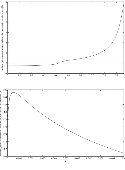
Figure 3: Welfare gains for different levels of nominal rigidities (η) and of financial market incompleteness (χ). 0 0.1 0.2 0.3 0.4 0.5 0.6 0.7 0.8 0.9 −2 0 2 4 6 8 10 12 η

welfare gains/losses related to financial markets incompleteness (%)

0 0.001 0.002 0.003 0.004 0.005 0.006 0.007 0.008 0.009 0.01 1.68 1.7 1.72 1.74 1.76 1.78 1.8 1.82 1.84 1.86 χ

which financial markets incompleteness becomes costly in terms of welfare. For the baseline calibration of the model, the threshold value corresponds to η = 0.4. These simulations also show that, when inflation is not too costly, the benefits associated with lower inflation rates through incomplete financial markets disappear. In such a case, just as in Benigno [2007], the costs of imperfect risk-sharing dominate the costs of price stickiness. Figure 3 also reports the welfare gains of financial markets incompleteness for varying values of portfolio management costs. Our results are clearly unsensitive to variations in the value of χ since welfare gains range from 1.85% to 1.69% when χ ranges from 0 to 0.01, which corresponds to an average annual interest rate premium ranging from nearly 0% to 4%.

(vi): The persistence parameter ρa has a negative impact on welfare gains associated with

incomplete financial markets. Higher persistence generates less incentives for agents to smooth the consequences of asymmetric shocks on their wealths and enhances their incentives to adjust permanently. As a consequence, the appeal of smoother consumption and hours and lower inflation disappears as shocks become more persistent.7

7

Conclusion

This paper has argued that financial market incompleteness leads to welfare gains in a monetary union subject to productivity shocks and sticky prices. This effect results from the fact that incomplete financial markets are associated with a reduction of the volatility of national inflation rates in a monetary union, even when the aggregate inflation rate is stabilized by the central bank. Lower national inflation rates are associated with higher levels of aggregate welfare since agents highly penalize inflation variations. Under complete financial markets, external adjustment to idiosyncratic shocks implies terms of trade movements but the current account does not play any role. Under incomplete financial markets, agents may use the current account to smooth the consequences of asymmetric shocks differently across countries. This possibility implies a smoother path for the terms of trade and national inflation rates, which increases welfare. For most plausible values of price stickiness, this effect dominates the welfare losses of imperfect risk-sharing associated with incomplete financial markets, that are consequently welfare dominant. We quantify the corresponding welfare gains to an average increase of 1.8% in permanent consumption.

7_{Our results are robust to several extensions, such as the introduction of demand shocks, exemplified in this}

References

Auray, S. and A. Eyquem, Public Spending Shocks and Welfare in a Monetary Union, 2007. mimeo.

Beetsma, R. and H. Jensen, Monetary and fiscal policy interactions in a micro-founded model of a monetary union, Journal of International Economics, 2005, 67 (2), 320–352.

Benigno, P., Price Stability with Imperfect Financial Integration, manuscript 2007.

and M. Woodford, Inflation Stabilization and Welfare: The Case of a Distorted Steady State, Journal of the European Economic Association, 2005, 3 (6), 1185–1236.

and , Optimal taxation in an RBC model: A linear-quadratic approach, Journal of

Economic Dynamics and Control, 2006, 30 (9–10), 1445–1489.

Calvo, G., Staggered Contracts and Exchange Rate Policy, in J. Frenkel, editor, The Economics

of Flexible Exchange Rates, Chicago: University of Chicago Press, 1983.

Canzoneri, M., R. Cumby, and B. Diba, The Cost of Nominal Inertia in NNS Models, Journal

of Money, Credit and Banking, 2006. Forthcoming.

Cole, H. and M. Obstfeld, Commodity trade and international risk sharing : How much do financial markets matter?, Journal of Monetary Economics, 1991, 28 (1), 3–24.

Corsetti, G., Openness and the Case for Flexible Exchange Rates, Research in Economics, 2006,

60 (1), 1–21.

Faia, E., Finance and International Business Cycles, Journal of Monetary Economics, 2007, 54 (4), 1018–1034.

Harrigan, J., OECD Imports and Trade Barriers in 1983, Journal of International Economics, 1993, 35 (1–2), 99–111.

Kim, J., S. H. Kim, and A. Levin, Patience, persistence, and welfare costs of incomplete markets in open economies, Journal of International Economics, 2003, 61 (2), 385–396.

, , and , Spurious Welfare Reversals in International Business Cycle Models,

Journal of International Economics, 2003, 60 (2), 471–500.

Lane, P. R. and G. M. Milesi-Ferretti, The External Wealth of Nations: Measures of Foreign Assets and Liabilities in Industrial and Developing Countries, Journal of International

Economics, 2001, 55 (2), 263–94.

Rotemberg, J. and M. Woodford, An Optimization-Based Econometric Framework for the Evaluation of Monetary Policy, in Bernanke Ben S. and Julio J. Rotemberg, editors, NBER

Macroeconomics Annual, 1997.

Schmitt-Grohe, S. and M. Uribe, Closing Small Open Economy Models, Journal of International

Economics, 2003, 61 (1), 63–85.

Woodford, M., Optimal Interest-rate Smoothing, Review of Economic Studies, 2003, 70 (4), 861–86.

Appendix

The natural equilibrium

We define the natural (Pareto-efficient) equilibrium as the economic equilibrium arising when prices are flexible under complete asset markets, i.e. ηh _{= η}f _{= 0 and χ = 0.}

We firstly derive the natural path of aggregate variables, defined as,

xu_t = 1 2 h xh_t + xf_t i .

Using the pricing equations, ph,t = wht − aht and pf,t= wft − aft, and adding them,

wu_t − pu_t = au_t.

Using the aggregate leisure-consumption arbitrage,

ψnu_t + ρcu_t = wu_t − pu_t,

the aggregate production function,

y_tu = au_t + nu_t,

and the aggregate equilibrium of goods markets,

y_tu= cu_t,

we get the natural path of the aggregate consumption, which also equals the aggregate output, e

y_tu= ecu_t = 1 + ψ

ρ + ψa

u t.

Combining the previous expression with the aggregate Euler equation, we determine the natural equilibrium interest rate,

δ 1 + δert+1= ρEt © e cu_t+1ª− ecu_t, implying, e r_t+1= ρ(1 + δ)(1 + ψ) δ(ρ + ψ) (Et © au_t+1ª− au_t).

We now turn to the natural path of relative variables, defined as,

xr_t = 1 2 h xf_t − xh_t i .

In the natural equilibrium, the financial market is complete, implying, 2ρecr_t = − (1 − 2α) est.

Combining this expression with the relative leisure-consumption arbitrage condition, we get,

ψenr_t −1 − 2α

2 est= ew

r t − eprt.

Using the definition of terms of trade, e

pr_t = (1 − 2α) 2 set, the relative leisure-consumption arbitrage condition becomes,

ψenr_t = ewr_t.

The relative pricing equation yields, e

st= epf,t− eph,t = 2 ( ewrt − eart) ,

which, combined with the previous condition, yields,

ψenr_t = 1

2set+ a

r

t. (19)

On the other hand, the risk-sharing condition, combined with the relative equilibrium con-dition on goods markets yields,

e

y_tr= −$αest,

where $α= (1−2α)

2_{+4ρµα(1−α)}

2ρ .

Using the relative production function, e

nr_t = eyr_t − ar_t,

we get,

e

nr_t = −$αset− art. (20)

Combining (19) and (20), we get the natural path of terms of trade, e

st= −_{(1 + 2ψ$}2 (1 + ψ) α)a

r t.

Summing up, using the relative equilibrium condition of goods markets to get ecr

t, and the relative

production function to get enr

t, we get, e st = −_{1 + 2ψ$}2 (1 + ψ) α ar_t, e cr_t = (1 + ψ) (1 − 2α) ρ (1 + 2ψ$α) a r t, e nr_t = 2$α− 1 (1 + 2ψ$α)a r t.

The quadratic welfare–based loss function

The welfare criterion writes,

ω_T = T X t=0 βtE₀ ½Z ₁ 0 · 1 2U h t (j) + 1 2U f t (j) ¸ dj ¾ = T X t=0 βtE0 ½Z ₁ 0 £ U_C,tu (j) − U_N,tu (j)¤dj ¾ .

After using the symmetry among agents, we get U_C,tu (j) = U_C,tu = 1 2 (1 − ρ) ³ C_th ´_1−ρ + 1 2 (1 − ρ) ³ C_tf ´_1−ρ , U_N,tu (j) = U_N,tu = 1 2 (1 + ψ) ³ N_th ´_1+ψ + 1 2 (1 + ψ) ³ N_tf ´_1+ψ .

We begin the derivation by taking a second order approximation of Uu N,t, U_N,tu ' N1+ψ 1 + ψ + N 1+ψ · nu_t +1 + ψ 2 ³ [nu_t]2+ [nr_t]2 ´¸ + O¡°°ξ3°°¢.

Recalling that the approximation is taken around the steady state assuming £ai t

¤₂

= 0 (see Benigno and Woodford [2005]), second order approximations of production functions write,

nh_t +1 2 h ah_t + nh_t i₂ = y_th+ dph_t + t.i.p + O¡°°ξ3°°¢, nf_t +1 2 h af_t + nf_t i₂ = y_tf + dpf_t + t.i.p + O¡°°ξ3°°¢,

where t.i.p gathers terms independent of the policy problem, and where,

dpi_t= θ

2var (pi,t) ,

implying £dpi_t¤2 ∈ O¡°°ξ3°°¢.

Combining these expressions, we get,

nu_t+1 2[n u t]2+ 1 2[n r t]2+ 1 2a h tnht+ 1 2a f tnft = yut+ 1 2[y u t]2+ 1 2[y r t]2+ θ 4var (ph,t)+ θ 4var (pf,t)+t.i.p+O ¡° °ξ3°_°¢_. The previous expression is then plugged in the approximation of Uu

N,t, U_N,tu ' N1+ψ{y_tu+ 1 2[y u t]2+ 1 2[y r t]2− 1 2a h tnht − 1 2a f tnft + θ 4var (ph,t) + θ 4var (pf,t) + ψ 2 [n u t]2+ ψ 2 [n r t]2} + t.i.p + O¡°°ξ3°°¢. Now focusing on Uu

C,t, we compute a second order approximation of UC,tu ,

U_C,tu ' C1−ρ 1 − ρ+ C 1−ρ · cu_t +1 − ρ 2 ³ [cu_t]2+ [cr_t]2 ´¸ + O¡°°ξ3°°¢.

A second order approximation of final goods markets equilibria gives,

y_th+1 2 h y_th i₂ = (1 − α) µ ch_t + µαs_t+1 2 h ch_t + αµs_t i₂¶ + α µ cf_t + µ (1 − α) s_t+1 2 h cf_t + µ (1 − α) s_t i₂¶ + t.i.p + O¡°°ξ3°°¢, y_tf+ 1 2 h y_tf i₂ = (1 − α) µ cf_t − µαst+1₂ h cf_t − µαst i₂¶ + α µ ch_t − µ (1 − α) st+1₂ h ch_t − (1 − µα) st i₂¶ + t.i.p + O¡°°ξ3°°¢.

Combining these expressions, we get, yu_t +1 2[y u t]2+ 1 2[y r t]2 = cut + 1 2[c u t]2+ 1 2[c r t]2+ µα (1 − α) 2 [st] 2 + t.i.p + O¡°°ξ3°°¢, or, cu_t +1 2[c u t]2+ 1 2[c r t]2 = yut + 1 2[y u t]2+ 1 2[y r t]2− µα (1 − α) 2 [st] 2 + t.i.p + O¡°°ξ3°°¢.

The previous expression is then plugged in the approximation of Uu C,t, U_C,tu ' C1−ρ{y_tu+1 2[y u t]2+ 1 2[y r t]2− µα (1 − α) 2 [st] 2₋ρ 2[c u t]2− ρ 2[c r t]2} + t.i.p + O ¡° °ξ3°_°¢_. Now combining Uu N,t and UC,tu , we get, U_tu = U_C,tu − U_N,tu ' C1−ρ{y_tu+ 1 2[y u t]2+ 1 2[y r t]2− µα (1 − α) 2 [st] 2₋ρ 2[c u t]2− ρ 2[c r t]2 − N1+ψ{yu_t +1 2[y u t]2+ 1 2[y r t]2+ θ 4var (ph,t) + θ 4var (pf,t) − 1 2a h tnht − 1 2a f tnft +ψ 2 [n u t]2+ ψ 2 [n r t]2} + t.i.p + O ¡° °ξ3°_°¢_. Using the fact that,

N1+ψ = Y AN ψ _{= Y C}−ρ _{= C}1−ρ_, we get, U_tu ' C1−ρ{−µα (1 − α) 2 [st] 2₋ρ 2 h [cu_t]2+ [cr_t]2 i +1 2a h tnht + 1 2a f tnft −ψ 2 h [nu_t]2+ [nr_t]2 i −θ 4var (ph,t) − θ 4var (pf,t)} + t.i.p + O ¡° °ξ3°_°¢_. Using, nu_t = y_tu− au_t, yu_t = cu_t, we get, U_tu' C1−ρ{−µα (1 − α) 2 [st] 2₋θ 4var (ph,t) − θ 4var (pf,t) − ρ 2[c u t]2− ρ 2[c r t]2− ψ 2 [n r t]2+ 1 2a h tnht + 1 2a f tnft − ψ 2 h [cu_t]2− 2cu_tau_t i } + t.i.p + O¡°°ξ3°°¢.

We then manage to make the term [cu_t − ecu_t]2 appear in the welfare criterion, we get, U_tu' C1−ρ 2 {−µα (1 − α) [st] 2₋θ 2var (ph,t) − θ 2var (pf,t) − (ρ + ψ) [cu_t − ecu_t]2− 2 (ρ + ψ) c_tuecu_t + 2ψcu_tau_t − ρ [cr_t]2− ψ [nr_t]2+ ah_tn_th+ af_tnf_t} + t.i.p + O¡°°ξ3°°¢.

Using the defintion of ecu t, e cu_t = 1 + ψ ρ + ψa u t, we get, U_tu' C1−ρ 2 {−µα (1 − α) [st] 2₋θ 2var (ph,t) − θ 2var (pf,t) − (ρ + ψ) [cu_t − ecu_t]2− 2 (1 + ψ) cu_tau_t + 2ψcu_tau_t − ρ [cr_t]2− ψ [nr_t]2+ ah_tn_th+ af_tnf_t} + t.i.p + O¡°°ξ3°°¢.

We then use the following relation,

ah_tnh_t + af_tnf_t = 2nu_tau_t + 2nr_tar_t, = 2cu_tau_t + 2nr_tar_t + t.i.p, to get, U_tu' C1−ρ 2 {−µα (1 − α) [st] 2₋θ 2var (ph,t) − θ 2var (pf,t) − (ρ + ψ) [cu_t − ecu_t]2− ρ [cr_t]2− ψ [nr_t]2+ 2nr_tar_t} + t.i.p + O¡°°ξ3°°¢.

In the next step, we show that 2nr

tart can be expressed as a function of est, ecrt, nrt. We start

with the following decomposition, 2nr_tar_t = 2 (1 + ψ) 1 + 2ψ$αn r tart + µ 2ψ 2$α− 1 1 + 2ψ$αa r t ¶ | {z } 2ψenr t nr_t. Using, nr_t = y_tr− ar_t, y_tr = (1 − 2α) cr_t− 2µα (1 − α) st,

and using natural equilibrium expressions of est, ecrt, enrt,

e st = −_{1 + 2ψ$}2 (1 + ψ) α ar_t, e cr_t = (1 + ψ) (1 − 2α) ρ (1 + 2ψ$α) a r t, e nr_t = 2$α− 1 (1 + 2ψ$α)a r t,

we get, 2nr_tar_t = 2cr_t µ (1 + ψ) (1 − 2α) (1 + 2ψ$α) ar_t ¶ | {z } ρecr t − 2µα (1 − α) s_t µ 2 (1 + ψ) 1 + 2ψ$α ar_t ¶ | {z } −est + 2ψenr_tnr_t+ t.i.p, or

2nr_tar_t = 2ρecr_tcr_t+ 2ψenr_tnr_t+ 2µα (1 − α) estst+ t.i.p.

Plugging this relation in the welfare criterion, we get,

U_tu ' C 1−ρ 2 {− θ 2var (ph,t) − θ 2var (pf,t) − µα (1 − α) [bst] 2 − (ρ + ψ) [bcu_t]2− ρ [bcr_t]2− ψ [bnr_t]2} + t.i.p + O¡°°ξ3°°¢,

where bxt= xt− ext are variables expressed in deviation to their natural equilibrium expressions.

Actualizing and summing, we get,

ω_T =

T

X

t=0

βtE₀{U_tu} .

Following Woodford [2003] we know that,

T X t=0 βtvar (pi,t) = T X t=0 βtπ 2 i,t ki , where ki ₌ (1−ηiβ)(1−ηi) ηi ,.

Finally, the welfare criterion criterion writes,

ωT = −C 1−ρ 2 T X t=0 βtEt{_2kθ_hπ2h,t+ θ 2kfπf,t2 + (ρ + ψ) [bcut]2 + µα (1 − α) [bs_t]2+ ρ [bcr_t]2+ ψ [bnr_t]2} + t.i.p + O¡°°ξ3°°¢,