Elections and de facto Expenditure Decentralization in Canada

Texte intégral

(1)2014s-28. Elections and de facto Expenditure Decentralization in Canada Mario Jametti, Marcelin Joanis. Série Scientifique Scientific Series. Montréal Avril 2014. © 2014 Mario Jametti, Marcelin Joanis. Tous droits réservés. All rights reserved. Reproduction partielle permise avec citation du document source, incluant la notice ©. Short sections may be quoted without explicit permission, if full credit, including © notice, is given to the source..

(2) CIRANO Le CIRANO est un organisme sans but lucratif constitué en vertu de la Loi des compagnies du Québec. Le financement de son infrastructure et de ses activités de recherche provient des cotisations de ses organisations-membres, d’une subvention d’infrastructure du Ministère de l'Enseignement supérieur, de la Recherche, de la Science et de la Technologie, de même que des subventions et mandats obtenus par ses équipes de recherche. CIRANO is a private non-profit organization incorporated under the Québec Companies Act. Its infrastructure and research activities are funded through fees paid by member organizations, an infrastructure grant from the Ministère de l'Enseignement supérieur, de la Recherche, de la Science et de la Technologie, and grants and research mandates obtained by its research teams. Les partenaires du CIRANO Partenaire majeur Ministère de l'Enseignement supérieur, de la Recherche, de la Science et de la Technologie Partenaires corporatifs Autorité des marchés financiers Banque de développement du Canada Banque du Canada Banque Laurentienne du Canada Banque Nationale du Canada Banque Scotia Bell Canada BMO Groupe financier Caisse de dépôt et placement du Québec Fédération des caisses Desjardins du Québec Financière Sun Life, Québec Gaz Métro Hydro-Québec Industrie Canada Intact Investissements PSP Ministère des Finances et de l’Économie Power Corporation du Canada Rio Tinto Alcan Transat A.T. Ville de Montréal Partenaires universitaires École Polytechnique de Montréal École de technologie supérieure (ÉTS) HEC Montréal Institut national de la recherche scientifique (INRS) McGill University Université Concordia Université de Montréal Université de Sherbrooke Université du Québec Université du Québec à Montréal Université Laval Le CIRANO collabore avec de nombreux centres et chaires de recherche universitaires dont on peut consulter la liste sur son site web. Les cahiers de la série scientifique (CS) visent à rendre accessibles des résultats de recherche effectuée au CIRANO afin de susciter échanges et commentaires. Ces cahiers sont écrits dans le style des publications scientifiques. Les idées et les opinions émises sont sous l’unique responsabilité des auteurs et ne représentent pas nécessairement les positions du CIRANO ou de ses partenaires. This paper presents research carried out at CIRANO and aims at encouraging discussion and comment. The observations and viewpoints expressed are the sole responsibility of the authors. They do not necessarily represent positions of CIRANO or its partners.. ISSN 2292-0838 (en ligne). Partenaire financier.

(3) Elections and de facto Expenditure Decentralization in Canada * Mario Jametti †, Marcelin Joanis ‡. Résumé/abstract This paper empirically investigates the underlying determinants of expenditure decentralization, based on the predictions of a new political economy model of partial decentralization. The analysis is based on an agency model, in which two levels of government are involved in the provision of a public good and voters are imperfectly informed about each government’s contribution to the good, creating a shared accountability problem. Under shared expenditure responsibility, the degree of decentralization is endogenous and depends on the relative political conditions prevailing at each level of government. Consistent with the model’s predictions, empirical results from a panel of Canadian provinces show that decentralization in a province increases with the electoral strength of the provincial government and decreases with the electoral strength of the federal government, in addition to being affected significantly by the partisan affiliation of both levels of government. A series of alternative empirical specifications, including an IV regression exploiting campaign spending data, are presented to assess the robustness of these results. Mots clés/Keywords: Fiscal decentralization, fiscal federalism, vertical interactions, partial decentralization, elections. Codes JEL : R50, H77, D72. *. For their comments on earlier drafts, we thank Toke Aidt, Jan Brueckner, Tom Crossley, Grégoire Rota Graziosi and Mark Schelker, in addition to seminar and session participants at WZB Berlin, Koç University (Istanbul), the JMA, the IIPF, the CEA and the SCSE. Financial support from the Swiss National Science Foundation (grants ProDoc - 130443 and Sinergia - 130648 and 147668) and Québec.s FRQSC is gratefully acknowledged. All remaining errors are our own. † Institute of Economics (IdEP), University of Lugano, Via G. Buffi 6, 6904 Lugano, Switzerland; e-mail: mario.jametti@usi.ch. Also affiliated with the Swiss Public Administration Network (SPAN). ‡ Corresponding author: Department of Economics, Université de Sherbrooke, Faculté d’administration, 2500 boul. de l’Université, Sherbrooke (Québec), Canada, J1K 2R1; e-mail: marcelin.joanis@usherbrooke.ca..

(4) 1. Introduction. Over the past decade, the Second Generation of …scal federalism theoretical models have deepened our understanding of the potential role that political economy considerations can play as determinants of the economic performance of decentralized systems (Weingast, 2009; Oates, 2005). As highlighted by Weingast (2009), a key feature of the Second Generation literature as opposed to the First Generation models is a focus on positive rather than normative predictions. This positive focus provides solid foundations for empirical research. One area of investigation for which Second Generation models open up especially promising perspectives is the study of the determinants of decentralization. There is indeed a well-documented global trend towards delegation of expenditure and revenue decisions to lower level governments, but the determinants of this trend remain surprisingly little explored. This may be (at least in part) the result of the essentially normative focus of the First Generation models of the ‘assignment problem.’ Much of that theoretical literature is indeed based on the “Decentralization Theorem”(Oates, 1972), that characterizes the trade-o¤ “between e¢ cient internalization of interjurisdictional spillovers through centralization and e¢ cient matching of local policies to local tastes through decentralization” (Epple and Nechyba, 2004, p. 2453). The related literature thus tends to treat the assignment decision as a binary one (centralization or decentralization). In reality, decentralization reforms are typically of partial nature, featuring provision of goods and services by intermediate levels of government (Seabright, 1996), by subnational governments that remain heavily dependent on transfers from the central government (Brueckner, 2009; Borge et al., 2014), by di¤erent levels of government in a given policy area (Joanis, 2014; Jametti and Joanis, 2009), or by local governments that provide and fund only some goods while others are provided centrally or internationally (Hart…eld and Padro i Miquel, 2012). Yet, the political economy of partial decentralization remains essentially unexplored in the empirical literature. This paper tests the empirical implications of a theory of ‘partial expenditure decentralization’ on the observed degree of decentralization. The model, adapted from Joanis (2014), is cast in the context of a pure moral hazard political agency model, an approach initiated by Barro (1973) and Ferejohn (1986). In the model, two levels of government are involved in the provision of a public good and voters are imperfectly informed about each government’s contribution to the good, creating a shared accountability problem. In most federations there is indeed, for many speci…c public tasks, overlap in spending duties between levels of government.1 Under such partial decentralization, policy outcomes are often the joint result of actions taken by politicians at di¤erent 1. A related literature studies overlapping soft budget constraints –see Breuillé and Vigneault (2010) for a theoretical. treatment and Baskaran (2012) for an empirical application.. 2.

(5) levels of government. The resulting joint accountability in public good provision has two important consequences, as highlighted by Joanis (2014): First, it gives rise to informational problems which may complicate the task faced by voters in disciplining politicians. Second, partial decentralization introduces vertical interactions between levels of government in public good provision.2 Together, these mechanisms imply that the degree of expenditure decentralization is an equilibrium outcome rather than a …xed institutional characteristic inherited, for instance, from decisions made at the constitutional table. The model’s main testable predictions pertain to the determinants of the degree of decentralization. Decentralization is endogenous and will depend, among other factors, on the relative political conditions prevailing at each level of government, i.e. the extent to which each level of government can a¤ect its electoral fortunes by contributing to the public good. The paper’s empirical endeavour is to test this prediction by estimating the e¤ect of political considerations on the de facto degree of (partial) expenditure decentralization. It is tested with data from a panel of Canadian provinces which has the key feature of compiling public spending by federal, provincial and local governments within each province. Canada, being one of the world’s most decentralized federations, displays ample cross-province heterogeneity and over-time variation in the observed degree of expenditure decentralization. Consistent with the model’s predictions, empirical results show that decentralization in a province increases with the electoral strength of the provincial government and decreases with the electoral strength of the federal government, together with being a¤ected signi…cantly by the partisan a¢ liation of both levels of government. The e¤ect of political variables and other controls are identi…ed within province and over time, with province …xed e¤ects included in all empirical speci…cations. This allows us to control for systematic di¤erences between provinces that may jointly in‡uence provincial politics and the degree of expenditure decentralization, such as the provincial-municipal …scal arrangements or the speci…city of a province’s political landscape. In addition, any common shock a¤ecting all provinces – such as federal policy – is controlled for by year …xed e¤ects in our baseline speci…cations. A series of alternative empirical speci…cations, including an IV regression exploiting campaign spending data, are presented to assess the robustness of our main results. This paper is related to a still fairly small empirical literature on the determinants of …scal decentralization, where decentralization is measured in terms of a revenue or expenditure ratio between di¤erent levels of government. An early, cross-sectional attempt is Panizza (1999), who …nds that country size, income, ethnic fractionalization and the degree of democracy all reduce 2. For vertical interactions in tax competition and in direct democracy, see e.g. Brülhart and Jametti (2006) and. Galletta and Jametti (2012).. 3.

(6) the degree of …scal centralization. Similar results are presented by Arzaghi and Henderson (2005), using a panel of countries. Jametti and Joanis (2011), also in a cross-country panel, explicitly consider political variables. In a within-country study, also in a panel context, on the determinants of decentralization in Switzerland Feld et al. (2008) show that centralization is negatively related to the availability of direct democratic decision-making (referenda), while Funk and Gathman (2011), using a longer panel, do not …nd such an e¤ect.3 To the best of our knowledge, our paper is the …rst to empirically test a political economy theory of the determinants of decentralization in a within-coutry panel, thus allowing us to introduce explicitly the e¤ects of political choices on the degree of decentralization while directly tackling the inherent endogeneity issues (through …xed e¤ects and IV regressions). The paper proceeds as follows. After a brief discussion of the Canadian context in Section 2, Section 3 lays down the theoretical model and derives empirically-testable predictions. Section 4 introduces the empirical strategy and the Canadian data, with empirical results being presented in Section 5. The last section concludes.. 2. The Canadian Institutional Context. We focus our attention on the period following Canada’s so-called ‘patriation’of the Constitution (from the UK) which led to the adoption of the Constitution Act of 1982. By international standards, Canada is a fairly decentralized federation, with the provinces exerting large areas of responsibility especially in the social policy sphere (e.g. health, education, social assistance). The 1982 patriation act was the country’s only comprehensive constitutional reform since the 1867 British North America Act. Before and after 1982, the de jure distribution of expenditure responsibilities has remained memarkably stable. Yet, Provincial Economic Accounts data (see details in Section 4.1) reveal that the level of de facto expenditure decentralization observed in a province is far from being a …xed institutional arrangement. It does indeed vary signi…cantly over time and across provinces. Since the early 1980s, the average share of provincial program spending in total program spending by all tiers of government in a given province was as low as 40.1% in Nova Scotia and as high as 60.0% in Alberta and 56.8% in Québec, see Table 1. New Brunswick exhibited the largest variability over the period, with a standard deviation of 2.89, while Nova Scotia and Québec were the most stable according to 3. Our paper is also related, but to a lesser extent, to the large body of empirical research investigating decentral-. ization as a determinant of various economic variables. For example, Oates (1985) relates the size of government to the degree of decentralization, a question that has been taken up by a number of studies (for a survey, see Feld et al., 2003).. 4.

(7) the same metric. While most provinces experienced an upward trend in the share of total spending by the provincial government, especially since the mid-1990s, an upward trend in decentralization over the entire period is less clear, with some provinces experiencing declines (e.g. Nova Scotia and British Columbia) in recent years –see the Appendix for province-by-province plots of the degree of decentralization over time. The respective roles of the federal and provincial governments give rise to recurrent and often heated debates. In particular, the involvement of the federal government in areas of provincial jurisdiction (through so-called ‘federal spending power’) is controversial, especially in the autonomyseeking province of Québec, and arguably leads voters to perceive most spending areas as areas that are de facto of shared responsibility. For example, Québec’s Commission on Fiscal Imbalance (2002, p. 127) notes that “in the administration of health care, a …eld of particular public concern, Canadians …nd it very di¢ cult to clearly identify the roles and responsibilities of each order of government. They seem to overestimate the …nancial contribution of the federal government and, more generally, do not seem to know exactly who is responsible for what.” We follow this view in the theoretical perspective exposed in the next section. Our political economy model of partial expenditure decentralization will guide our empirical investigation by capturing in a stylized way a key aspect of (Canadian) federalism: A …xed constitutional order from which the observed de facto degree of decentralization may ‘deviate’over time and within province as a result of an ongoing political game played between the federal and provincial governments.. 3. A Model of Shared Responsibility in a Federation. This section, adapted from Joanis (2014), lays down a model in which a public good valued by the voters in a given jurisdiction is jointly provided by two levels of government (labelled ‘federal’and ‘provincial’).4 It describes the environment (composed of two governments and N identical voters) and derives key results on the political determinants of decentralization. In each of two periods, two levels of government choose …scal policy (taxes collected and spending) to maximize their expected level of rent extraction, subject to the constraint that they need to seek reelection at the end of the …rst period. Voters, who value public goods, can observe total taxes and can infer total rents. However, they do not observe the intergovernmental composition of expenditures and taxes. Public good provision is positively related to the reelection probability of both governments such that the spending decisions of one level of government a¤ects not only its 4. While the labels ‘federal’ and ‘provincial’(or its equivalent ‘state’) correspond best to the Canadian context of. this paper, the applicability of the model is much more general.. 5.

(8) own reelection probability but that of the other level of government as well (a positive externality arises). Each level of government’s equilibrium contribution to the public good equates its own marginal bene…t from reelection –with an incentive to free-ride on the other level of government’s contribution –to the marginal cost of foregone rents in the …rst period, taking as given the strategy of the other level of government.. 3.1. The Environment. Every period, the federal government (indexed by superscript f ) and the provincial government (indexed by superscript p) each contribute to the provision of a public good g in a province. Government j produces g j. 0 units of a publicly-provided input. Together, the federal and. provincial inputs are converted into a public good g by a constant elasticity of substitution (CES) technology:5 g= where. < 1:. p. and. f. f. (g f ) +. p. (g p ). 1=. ;. (1). are parameters that denote each level of government’s ‘competence’(e.g.. as de…ned by the constitution). Each government levies a lump-sum tax (T j ) and faces a common unit cost of production (~). Politicians in o¢ ce can divert tax revenues away from public good provision and towards their own bene…t. Assuming balanced budgets at each level of government, any of the jurisdiction’s N individuals faces a total tax bill of T = T f + T p = (g f + g p ) + sf + sp ; where. (2). = ~=N and sj are the per capita rents extracted by government j.. All individuals have the following quasi-linear utility function: u(g; z) = h(g) + z;. (3). where z denotes the consumption of a private good and h is a well-behaved concave function. For tractability, let us assume a simple functional form for h : h(g) = g ; where 0 <. (4). < 1. Furthermore, every period each individual is endowed with y units of the private. good such that z + T = y: 5. Nishimura (2006) also uses such an aggregation technology in a similar context.. 6. (5).

(9) Without loss of generality, we normalize the population of the jurisdiction to unity (N = 1) since all individuals are identical. For simplicity, let us make a few additional assumptions about taxes. Since taxes are lump-sum in this model, we can assume that individuals and governments take total taxes collected (T p and T f ) as given. Let us further assume that T p and T f are …xed at some pre-determined levels that are su¢ cient for each level of government to provide some arbitrary level of the public good (g). In sum, we assume the following series of inequalities for each government j: g. Tj. y:. (6). Let us de…ne the ‘degree of decentralization’ (d) as the share of provincial spending in total spending: d. 3.2. gf. gp 2 [0; 1]: + gp. (7). Introducing Politics: Opportunistic Politicians and Strategic Voters. Unless governments are assumed to be benevolent social planners, their behaviour depends on the incentives provided by the political process. This paper considers a two-period model, with separate elections taking place at the provincial and federal levels between the two periods. As in Besley and Smart’s (2006, 2007) political agency model, elections in our model can act as an imperfect disciplinary device.6 Politicians Each government maximizes expected discounted rents (per capita) over the two periods, given by S j = sj1 + P j sj2 ; where subscripts indicate periods,. (8). 2 [0; 1] is a discount factor and P j is incumbent j’s perception. of his reelection probability. Voters and elections Voters face a simple binary reelection decision in the elections held at the two levels of government at the end of period 1. The two elections are assumed to take place simultaneously.7 Furthermore, following Besley and Smart (2006), voters are taken to be able to announce and commit to a reelection rule before the elections take place. 6. See also Kessing’s (2010) related model, who also studies federalism and accountability but not partial decentral-. ization. 7 A case in which this assumption is relaxed is presented in Joanis (2009).. 7.

(10) Information The information available to voters at election time is crucial to the ability of elections to act as disciplinary devices. Two sources of imperfect information will be essential to the analysis that follows: 1. Voters do not observe the contribution of each level of government to the shared public good. However, voters observe the aggregate level of the public good. In other words, voters observe g but not g f and g p . 2. Uncertainty about the election outcome is introduced and resolved only after incumbents have taken all relevant decisions and just before the voters cast their ballots. From the point of view of incumbents, elections are ‘probabilistic.’ In the spirit of probabilistic voting models, such as those developed by Persson and Tabellini (2000) or more recently by Alesina and Tabellini (2007, 2008), election results are typically uncertain from the point of view of politicians (at least to some extent) since a series of shocks may a¤ect the electorate’s decision beyond …scal policy (e.g. other issues arising during the campaign, characteristics of challengers, partisan loyalty). Here, these shocks are speci…c to a given level of government, introducing heterogeneity in the electoral conditions between the elections taking place at the two levels of government. Timing. The timing of the game is as follows:. 1. Incumbents set period-1 …scal policy (determining the contribution to the shared public good and the level of rents); 2. Voters observe the realization of two random variables which summarize the electoral conditions speci…c to each election; 3. The federal and provincial elections take place; and 4. If reelected, the incumbents set period-2 …scal policy. Otherwise, voters achieve the utility level associated with challengers (similar in all respects to incumbents).. 3.3. Equilibrium and Theoretical Prediction. Voters announce that they will reelect each incumbent if their period-1 utility level exceeds some random threshold value,8 the distribution of which is assumed to be common knowledge. The cuto¤ utility level relevant to the provincial election is denoted u and is a random variable distributed 8. One interpretation for this is that information about some characteristics of the challengers becomes available. just before the election.. 8.

(11) according to F; a c.d.f. Hence, voters reelect the provincial government if u(g; T ). u:. (9). Symmetrically, they reelect the federal government if their utility exceeds the realization of a random variable v; distributed according to G; a c.d.f. From the point of view of incumbents, reelection is probabilistic. Electoral results depend on aggregate public good provision and on the realization of the stochastic reservation utility levels. The probability that the provincial incumbent is reelected is P p = Pr [u(g; T ). u] = F [u(g; T )] :. (10). For simplicity, let us assume that u is uniformly distributed on the interval [0; u ], implying that Pp =. 1 u(g; T ): u. (11). Note that the reelection probability is decreasing in u , the upper bound on the random cut-o¤ utility level. Hence, the election is riskier from the incumbent’s point of view the higher is this upper bound. We can now consider the provincial incumbent’s problem in period 1: max Tp p g. gp + T p. 1 u. ( f (g f ) +. p. (g p ) ). =. Tp. Tf ;. (12). which is obtained by substituting the government’s budget constraint ( g p + sp = T p ) and equation (11) in equation (8).9 The federal government solves a symmetric problem, with v. U [0; v ] : The. two levels of government are assumed to behave non-cooperatively in setting their contribution to the public good, taking the contribution level of the other government as given. Since elections are simultaneous, the equilibrium contribution levels in period 1 will be those observed in a Nash equilibrium. Under shared responsibility, the degree of decentralization is endogenous and is the outcome of vertical interactions between the two levels of government that are shaped by the degree of substitutability between the public inputs.10 The reaction functions are given by: Tp f f ( (g ) + u Tf f f ( (g ) + v 9. (g p ) ). 1. (g p ) ). 1. p. p. (g p ). 1 p. =. ;. (13). (g f ). 1 f. =. :. (14). Time subscripts are dropped from now on since the period-2 problem is trivial, with maximum rents being taken. by each government. All decision variables relate to period 1. See Joanis (2014) for a discussion. 10 Whereas high complementarity mitigates the ability of each government to merely free-ride on the other’s contribution, complementarity is also associated with a more indirect e¤ect of aggregate spending on reelection probabilities.. 9.

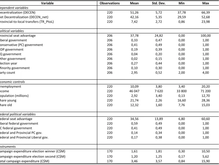
(12) Solving (13) for an interior solution yields the Nash equilibrium spending ratio: gp = gf. p f. Tp v Tf u. 1 1. ;. (15). which allows us to formulate the following proposition. Proposition 1 (Endogenous decentralization) The equilibrium spending ratio is determined by the product of three ratios: the relative competencies relative reelection uncertainties. v u. p f. , the revenue ratio. Tp Tf. , and the. .. The theoretical model thus leads to the following empirically-relevant equation: dj = f (. v )j ; Xj + "j ; u. where X is a vector of economic and political controls –encompassing the. (16) j. and T j parameters but. including other determinants of decentralization not explicitly modelled – and " is an error term. In the remainder of this paper, we develop an empirical implementation of this equation. Our main endeavor is to identify the e¤ect of electoral conditions on the observed degree of decentralization. Recall that u and v capture the uncertainty of the election at each level of government. When u (v ) increases, the reelection prospects of the provincial (federal) incumbent become more uncertain. Ceteris paribus, in the model, this reduces the incumbent’s incentive to spend on the public good.. 4. Data and Descriptive Statistics. To implementing equation (16) empirically we assembled data from three sources: (i) Provincial Economic Accounts data that will allow us to calculate within-province federal-provincial expenditure decentralization, (ii) elections data, and (iii) data on economic and demographic provincial characteristics. Summary statistics for all variables used in the analysis are provided in Table 2.. 4.1. Decentralization. To measure the degree of decentralization, our main dependent variable, we use data from Statistics Canada’s Provincial Economic Accounts for the 1981-2006 period.11 For our purposes, a crucial feature of the Provincial Economic Accounts is that they record spending by the federal, provincial and local governments within each province. We de…ne our decentralization variable (DECEN ) as the ratio of provincial program spending (i.e. excluding debt charges) to consolidated program 11. 2006 marks a natural break-point in electoral data at the federal level, marking the end of an era of Liberal. governments (since 1993) and major changes to the Canada Elections Act (with the adoption of Bill C-16).. 10.

(13) spending in the province (i.e. federal, provincial and local spending).12 Our data will allow us to further ‘decompose’ the decentralization variable in order to isolate the portion of provincial spending that consists of provincial transfers to local governments, a component that will prove to be especially sensitive to electoral conditions.13 This decomposition will supply a ‘net decentralization’ ratio (DECEN _net) calculated as the ratio of provincial program spending net of provincial-tolocal transfers to consolidated program spending. It will also supply a measure of the relative size of provincial transfers to local governments (T R_P toL), which we will express as a share of total program spending by the provincial government. All three variables will be used as dependent variables in the regression analysis of the next section.14 Table 2 reveals that the average degree of decentralization of program spending was 51.3%, with a minimum at 37.8% and a maximum at 66.4%. Program spending includes an average of 7.4% of total spending attributable to provincial transfers to local governments, a variable for which there are wide di¤erences across provinces and over time (the standard deviation is 2.7). Net of provincial transfers to local governments, the average decentralization drops to 42.2%, with an observation as low as 29.6%. See the Appendix for province-by-province plots of DECEN and T R_P toL.. 4.2. Elections. The electoral variables are constructed from data obtained directly from the o¢ ces of provincial chief electoral o¢ cers. The sample consists of 63 provincial general elections held between 1985 and 2006, together with data on the seven federal elections held between 1984 and 2006.15 From the electoral data, three variables capturing provincial electoral conditions are extracted. First, the “seat advantage” measures the di¤erence between the government’s number of seats in the provincial legislature after the general election and the number of seats won by the second-place party, as a ratio of the total number of seats in the legislature – it is our preferred variable to capture (the inverse of) the theoretical model’s reelection uncertainty parameters (u and v ). It is intended to capture the electoral strength of the party in power (GOV ST REN ) and will be labeled as such in what follows. 12. Program spending can be decomposed into four components: public goods and services, transfers to individuals,. transfers to businesses and transfers to governments. 13 Transfers to local governments, which are targetable on a geographical basis, are well-known for their sensitivity to political economy consideration. See, for example, Case’s (2001) in‡uential paper. 14 Note that provincial transfers to the federal government (very small amounts) are always excluded from our measure provincial program spending. In Canada, as local governments are creatures of provincial governments and are not considered by the Constitution as a full-‡edged order of government, the bulk of transfers to local governments originate from the provincial governments. 15 The source for federal elections data is electionalmanac.com.. 11.

(14) We included a set of additional control variables. The “minority government” variable is a dummy equal to one if the number of seats won by the government party falls below 50% of the total number of seats. The “party count” variable reports the number of parties with at least one seat in the provincial legislature. In addition, we coded the partisan a¢ liation of the government party using a series of dummies. In the regressions, we always omit the (Center-Left) Liberal party dummy. The vector of provincial party dummies is denoted by PARTY. We constructed similar variables at the federal level (F ED_GOV ST REN , FED_PARTY). Dummy variables capturing the partisan alignment of the provincial and federal governments in a province (BOTH_PARTY) and a provincial election year dummy will also be included. In the dataset, we observe each province (denoted by i) every year (denoted by t) starting with the …rst election for which we collected data, and electoral variables are deemed unchanging between two elections. In the provinces, Conservative governments (Right) were in power 40.8% of the time in the period covered by the data, followed by Liberal governments (33%), New Democratic (NDP, Left) governments (19%), Parti Québécois (PQ, a separatist party) governments (4%, only in Québec), and other parties (2%).16 The average seat advantage was 37.8%, exhibiting wide variations (the standard deviation is 24.8 percentage points, with observations at 0% and 100%). Minority governments were in power 10.2% of the time, while the average number of parties in the provincial legislatures was 2.9 (varying between 2 and 4). At the federal level, the Conservatives served between 1984 and 1993, and from 2006 on, while the Liberals were in o¢ ce from 1993 to 2006. The Liberal government elected in 2004 and the Conservative government formed in 2006 were minority governments. Finally, to construct the instruments that will be used in Section 5.2, we collected data from provincial chief electoral o¢ cers on provincial electoral spending of the winning party, the challenger party as well as total campaign spending.. 4.3. Economic and Demographic Controls. Finally, we obtain yearly provincial demographic and economic controls from Statistics Canada’s CANSIM II database. The variables included in the X vector are the standard determinants of government spending and revenue, and as such they should be included as controls in decentralization regressions: 1. A province’s total population is a key driver of expenditures on many government services; 16. These other parties are British Columbia’s Social Credit Party and the Saskatchewan Party, both located on the. right of the political spectrum.. 12.

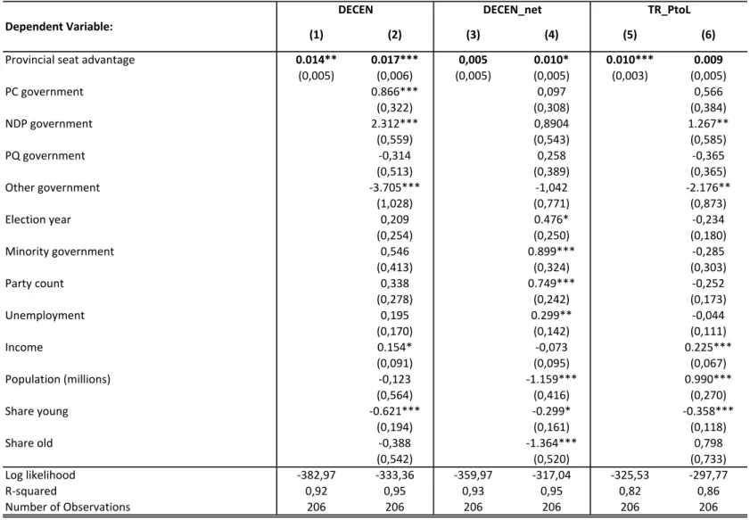
(15) 2. The elderly population (65 and over) is a determinant of spending on health care (the most expensive provincial responsibility) and old age pensions (a major federal responsibility); 3. The youth population (up to 15 years of age) is the primary determinant of spending on education (a provincial responsibility); 4. The unemployment rate is a determinant of spending on unemployment insurance (a federal program) and social assistance (provincial programs); and 5. Average household income is key driver of a government’s revenue-raising capacity. The next section is devoted to our empirical strategy and results.. 5. Empirical Implementation and Results. Our empirical strategy relies on equation (16), the main prediction derived from the theoretical model. A key relationship highlighted by this equation is the positive association between decentralization and provincial electoral strength (the inverse of u in the theoretical model). The Appendix provides a …rst glance into this relationship by presenting graphs for the seat advantage variable, decentralization of program spending and provincial transfers to local governments, for all ten provinces. The seat advantage series are easily recognizable by their step-wise shape. Interestingly, government strength (as measured by the seat advantage) matches closely the trend in decentralization and local transfers in many instances. For program spending, the cases of Newfoundland-and-Labrador, Prince Edward Island, Québec, Ontario and Alberta are noteworthy. Transfers to local governments appear to be especially sensitive to government strength in New Brunswick, Québec and Saskatchewan. In order to move beyond these unconditional correlations, the remainder of this section is structured around four sets of regression results. First, baseline results focus on the relationship between the provincial government’s electoral strength and decentralization within a province. Second, taking into account that the “seat advantage” variable is constant between elections, we present results clustering standard errors over the electoral cycle. Next, a series of IV results are then provided to deal with endogeneity issues. Finally, in a last set of results we introduce both provincial and federal politics as determinants of decentralization –these results are presented separately as they demand that year e¤ects are dropped in favor of the inclusion of a time trend. Regression results are presented in tables 3 to 6, which are similarly structured around six speci…cations, two pertaining to each of our three dependent variables: decentralization, decentralization net of provincial-to-local transfers, and the share of provincial-to-local transfers (see Section 4.1 above 13.

(16) for details). For each dependent variable, we present both a bivariate regression involving only the provincial seat advantage variable (capturing government strength) and a multivariate regression including all the relevant controls.. 5.1. Baseline Results. We …rst implement the following linear version of equation (16): DECENjt =. + GOV ST RENjt + PARTYjt + Xjt + PROVj + YEARt + "jt ;. (17). where PROVj is a vector of province …xed e¤ects, and YEARt is a vector of year …xed e¤ects. A constant is always included, though unreported. Liberal is the omitted party. Table 3 presents the …rst set of results based on this equation with robust standard errors.17 The multivariate Speci…cation 2 shows a positive and signi…cant (at the 1% con…dence level) e¤ect of provincial government strenght on decentralization, as predicted by the theoretical model: the observed degree of decentralization is higher when the provincial government is stronger. An increase of 10 percentage points in the seat advantage is associated with a 0.17-point increase in the decentralization ratio. There is also a strong estimated e¤ect of governments from the New Democratic Party and (perhaps surprisingly) the Conservative Party, which are associated with a decentralization ratio of as much as 2.07 points higher than Liberal governments. Governments of the B.C. Social Credit and the Saskatchewan Party (the ‘other parties’) are together associated with much lower decentralization levels. PQ governments do not signi…cantly di¤er from Liberal governments. Majority governments and the number of parties do not have a signi…cant e¤ect on decentralization. Interestingly, only one non-political control is statistically signi…cant. A province’s population share of youth is negatively correlated with decentralization. This is somewhat counter-intuitive given the provinces’ role in education. Yet, this result is probably a by-product of the complex e¤ect of population aging on the respective roles of the provinces (responsible for health care) and the federal government (responsible for old age security), especially when estimating the e¤ect of the youth share conditional on the population share of the elderly. Turning now to the decomposition of the decentralization ratio between the share of provincialto-local transfers (Speci…cations 5 and 6) and a decentralization ratio net of those transfers (Speci…cations 3 and 4), both dependent variables are also positively correlated with provincial government 17. We do not present results with standard errors clustered at the province level, since we only avail of 10 clusters. (see Wooldridge, 2003, for a discussion).. 14.

(17) strength, the positive and signi…cant coe¢ cient on the net decentralization ratio con…rming the robust e¤ect of government strength on decentralization estimated in Speci…cations 1 and 2. Furthermore, Speci…cation 4 displays signi…cant coe¢ cients for the minority government and party count variables, with the expected signs. Majority governments (at the provincial level) are associated with a decentralization ratio that is .86 points higher than minority governments. Finally, a divided opposition is also associated with a higher decentralization ratio: an additional party in the provincial legislature translates into a .75-point increase in decentralization. These two e¤ects work in the same direction as the e¤ect of the seat advantage variable, indicating a positive relationship between decentralization and provincial government strength. While the partisan e¤ects are not signi…cant, the coe¢ cient on the provincial election year dummy is now signi…cant (at the 10% level) and positive. The pattern for the economic controls are somewhat di¤erent in Speci…cation 4 relative to Speci…cation 2. Here, (net) decentralization is positively correlated with the unemployment rate, and a province’s population size is negatively correlated with decentralization, with a similar relationship holding for the senior population share –consistent with the federal government’s role in old age security. Regarding the …nal set of baseline results pertaining to provincial transfers to local governments –reported in Speci…cations 5 and 6 –in addition to a positive (albeit insigni…cant, when including controls) e¤ect of the seat advantage, the party dummies for the NDP and ‘other’governments are signi…cant (with signs consistent with Speci…cation 2). Three of the economic and demographic controls have a signi…cant e¤ect here: transfers increase with average family income and with a province’s population, but they decrease with the population of age 15 and younger. The results of a robustness check are reported in Table 4, dealing with potential issues with the estimation of standard errors given that electoral variables vary only once per electoral cycle while the dependent variable varies on a yearly basis. To adress this problem, standard errors in Table 4 are clustered on electoral cycles. Everything else in Table 4 is the same as in Table 3. Comparing the results in both tables reveals an una¤ected pattern of statistical signi…cance, with only a few minor exceptions. In particular, the results highlight the robustness of the positive e¤ect of a high provincial seat advantage (a strong provincial government) on expenditure decentralization in the province.. 5.2. Endogeneity. Table 5 displays the second-stage results of an IV regression in which the seat advantage is instrumented. We use electoral campaign spending variables as instruments for the seat advantage. Indeed, government strength and spending decisions are likely to be jointly determined. The iden15.

(18) tifying assumption here is that campaign spending has a direct e¤ect on electoral outcomes, but does not a¤ect directly public expenditure decisions and thus the degree of decentralization. The seat advantage is instrumented with campaign spending by the winning party, spending by the challenger party as well as total campaign spending in the province. The logs of the instruments are used to allow for decreasing returns on campaign spending. With respect to the e¤ect of the provincial seat advantage, the IV results con…rm the previous results for the main decentralization variable (i.e. Speci…cation 2 in Table 3). The magnitude of the seat advantage coe¢ cient is now higher, likely revealing a downward bias in the OLS estimates. The …rst stage results are provided in the Appendix. While the seat advantage coe¢ cient is still signi…cant in Speci…cation 3 (bivariate regression) with the net decentralization measure, it is not signi…cant when the control variables are added to the regression (Speci…cation 4). In the last two speci…cations (local transfers as the dependent variable), the IV results do not con…rm a positive and signi…cant sign for the seat advantage coe¢ cient. We would argue that using electoral campaign spending is a sound identi…cation strategy to address the endogeneity of decentralization and political strength. Our identifying assumption, that campaign spending does not directly a¤ect the decentralization ratio is con…rmed by the test for overidentifying restrictions, where the null hypothesis cannot be rejected in all our multivariate speci…cations (columns 2, 4 and 6). However, our IV results need to be taken with prudence, since we cannot exclude the possibility that our instruments are weak. Indeed, in the multivariate speci…cations we only reject the null that the set of instruments is weak at a 30% maximal IV relative bias (see Stock and Yogo, 2002). In our opinion, this is due to the fact that we avail of limited time-variation of the instruments in our sample, as campaign spending is only reported for elections and remains constant between them. This is also the reason why we present the IV results as a robustness check to our preferred Table 3 results.. 5.3. Relative Reelection Uncertainties. Finally, our ‘full model’adds federal electoral variables to equation (17): DECENjt =. + GOV ST RENjt + F ED_GOV ST RENt + PARTYjt + FED_PARTYt + BOTH_PARTYjt + Xjt +PROVj + t + ujt :. (18). The Liberals are again the omitted party, at both the provincial and the federal levels. Because the variables capturing federal politics do not vary across provinces, a time trend is included instead 16.

(19) of the year e¤ects included in all the other speci…cations discussed above. A dummy for a federal Conservative government and party alignment dummies are included. As for the previous tables, results for our main decentralization variable are reported in Speci…cations 1 and 2 of Table 6. Generally speaking, the baseline results are una¤ected by the inclusion of federal elections variables, with the noteworthy exception that the Conservative dummy is now insigni…cant. A high federal government seat share has the expected negative e¤ect on decentralization. Both the provincial and the federal seat advantages are signi…cant in Speci…cation 2. The alignment of Conservative governments at the federal and provincial levels increases the level of decentralization, perhaps indicating that provincial Conservatives have been less successful at constraining government size than federal Conservatives. A Liberal alignment has no e¤ect on decentralization. For decentralization net of provincial-to-local transfers, while the federal seat advantage is signi…cant in Speci…cation 3, it is not when controls are included in the regression. The provincial seat advantage is also insigni…cant in speci…cations 3 and 4. Finally, as expected, the federal electoral variables have no explanatory power when the dependent variable is the share of provincialto-local transfers in total provincial spending.. 6. Conclusion. Our empirical results lend support to the key prediction of our theoretical model of partial expenditure decentralization, which states that a strong provincial government relative to the federal government should lead to more decentralization. In our preferred speci…cation (Table 2) we have shown that decentralization in a province increases with the electoral strength of the provincial government, relative to the electoral strength of the federal government (captured by the year effects). These results are con…rmed by (i) explicitly considering the federal electoral strength (Table 6), and (ii) instrumenting electoral strength with campaign spending (Table 5). Albeit statistically signi…cant, the e¤ect of electoral strength on decentralization is small. Indeed, in our preferred speci…cation, a 10 percentage points increase in the seat advantage is associated with a 0.17- percentage point increase in the decentralization ratio. It should be noted that this is consistent with the fact that our theoretical model implies that politics is important at the margin. It is also consistent with the fact that the bulk of expenditure is attributed to levels of government through the constitutional assignment of tasks (which is controlled for by the province and year …xed e¤ects). Further, the observed degree of decentralization is also a¤ected signi…cantly by partisan a¢ lia-. 17.

(20) tions at both levels of government, and the partisan alignment of both levels of government. Taken together, our results supply strong evidence that electoral variables do belong in a comprehensive theory of the determinants of …scal decentralization. The analysis can most certainly be improved along some dimensions. An interesting avenue would be to explicitly include the ‘relative competencies’in the empirical analysis, perhaps using Public Sector E¢ ciency (PSE) measures –see, for example, Afonso et al. (2005).. 18.

(21) References [1] Afonso, Antonio, Ludger Schuknecht and Vito Tanzi (2005). Public Sector E¢ ciency: an International Comparison, Public Choice, 123, 321-347. [2] Alesina, Alberto and Guido Tabellini (2007). “Bureaucrats or Politicians? Part I: A Single Policy Task,” American Economic Review, 97, 169-179. [3] Alesina, Alberto and Guido Tabellini (2008). “Bureaucrats or Politicians? Part II: Multiple Policy Tasks,” Journal of Public Economics, 92, no. 3-4, 426-447. [4] Arzaghi, Mohammad and J. Vernon Henderson (2005). “Why Countries are Fiscally Decentralizing?” Journal of Public Economics, 89, 1157-1189. [5] Barro, Robert (1973). “The Control of Politicians: An Economic Model,” Public Choice, 14, 19-42. [6] Baskaran, Thushyanthan (2012). “Soft budget constraints and strategic interactions in subnational borrowing: Evidence from the German States, 1975–2005,”Journal of Urban Economics, 71(1), 114-127. [7] Besley, Timothy and Michael Smart (2006). “Political Agency and Public Finance,”in Timothy Besley, Principled Agents? The Political Economy of Good Government, Oxford University Press: Oxford, pp. 174-227. [8] Besley, Timothy and Michael Smart (2007). “Fiscal Restraint and Voter Welfare,” Journal of Public Economics, 91, 755-773. [9] Borge, Lars-Erik, Jan K. Brueckner and Jorn Rattsø (2014). “Partial Fiscal Decentralization and Demand Responsiveness of the Local Public Sector: Theory and Evidence from Norway,” Journal of Urban Economics, 80, 153-163. [10] Breuillé, Marie-Laure and Marianne Vigneault (2010). “Overlapping soft budget constraints,” Journal of Urban Economics, 67(3), 259-269. [11] Brueckner, Jan K. (2009). “Partial …scal decentralization,” Regional Science and Urban Economics, 39(1), 23-32. [12] Brülhart, Marius, and Mario Jametti (2006). “Vertical versus horizontal tax externalities: An empirical test,” Journal of Public Economics, 90(10-11), 2027–2062.. 19.

(22) [13] Case, Anne (2001). “Election goals and income redistribution: Recent evidence from Albania,” European Economic Review, 45, 405-423. [14] Commission on Fiscal Imbalance (2002). A New Division of Canada’s Financial Resources, Report, Government of Québec. [15] Epple, Dennis and Thomas Nechyba (2004). “Fiscal Decentralization,”in J. Vernon Henderson and Jacques-Françcois Thisse (Eds.), Handbook of Regional and Urban Economics Vol 4 - Cities and Geography, Elsevier - North Holland. [16] Feld, Lars P., Gebhard Kirchgässner and Christoph A. Schaltegger (2010). “Decentralized Taxation and the Size of Government: Evidence from Swiss State and Local Governments,” Southern Economic Journal, 77, 27-48. [17] Feld, Lars P., Christoph A. Schaltegger and Jan Schnellenbach (2008). “On Government Centralization and Fiscal Referendums,” European Economic Review, 52, 611-645. [18] Ferejohn, John (1986). “Incumbent Performance and Electoral Control,” Public Choice, 50, 5-25. [19] Funk, Patricia, and Christina Gathmann (2011). “Does direct democracy reduce the size of government? New evidence from historical data, 1890–2000,” Economic Journal 121(557), 1252-1280. [20] Galletta, Sergio and Mario Jametti (2012). “How to Tame two Leviathans? Revisiting the E¤ect of Direct Democracy on Local Public Expenditure,” CESifo working paper 3982. [21] Hart…eld, John W. and Gerard Padro i Miquel (2012). “A Political Economy Theory of Partial Decentralization,” Journal of the European Economic Association, 10(3), 605-633. [22] Jametti, Mario and Marcelin Joanis (2009). “The Rise of Partial Decentralization and Shared Responsibility Federalism”, in Núria Bosch et Albert Solé (ed.), World Report on Fiscal Federalism ’09, Institut d’Economia de Barcelona. [23] Jametti, Mario and Marcelin Joanis (2011). “Electoral Competition as a Determinant of Fiscal Decentralization,” CESifo working paper 3574. [24] Joanis, Marcelin (2009). “Intertwined Federalism: Accountability Problems under Partial Decentralization,” CIRANO working paper 2009s-39.. 20.

(23) [25] Joanis, Marcelin (2014). “Shared Accountability and Partial Decentralization in Local Public Good Provision,” Journal of Development Economics, 107, 28-37. [26] Kessing, Sebastian G. (2010). “Federalism and Accountability with Distorted Election Choices,” Journal of Urban Economics, 67, 239-247. [27] Nishimura, Yukihiro (2006). “Human Fallibility, Complementarity, and Fiscal Decentralization," Journal of Public Economic Theory, 8(3), 487-501. [28] Oates, Wallace E. (1972). Fiscal Federalism, New York: Harcourt Brace. [29] Oates, Wallace E. (1985). “Searching for Leviathan: An Empirical Study,”American Economic Review, 75, 748-757. [30] Oates, W. E. (2005). “Toward a Second-Generation Theory of Fiscal Federalism,”International Tax and Public Finance, 12, 349-373. [31] Panizza, Ugo (1999). “On the Determinants of Fiscal Centralization: Theory and Evidence,” Journal of Public Economics, 74, 97-139. [32] Persson, Torsten and Guido Tabellini (2000). Political Economics: Explaining Economic Policy, Cambridge: MIT Press. [33] Seabright, Paul (1996). “Accountability and Decentralisation in Government: An Incomplete Contracts Model,” European Economic Review, 40, 61-89. [34] Stegarescu, Dan (2009). “The e¤ects of economic and political integration on …scal decentralization: evidence from OECD countries,” Canadian Journal of Economics, 42(2), 694-718. [35] Stock, James H. and Motohiro Yogo (2002). “Testing for Weak Instruments in Linear IV Regression,” NBER Working Papers 0284. [36] Weingast, B. R. (2009). “Second Generation Fiscal Federalism: The Implications of Fiscal Incentives,” Journal of Urban Economics, 65, 279-293. [37] Wooldridge, Je¤rey M. (2003). “Cluster-Sample Methods in Applied Econometrics,”American Economic Review, (93(2), 133-138.. 21.

(24) Appendix: Graphs. 1995 year. 60. 20 40 govseatadv_share 52. Nova Scotia. 1995 year decen_op. govseatadv_share. 2000. 2005. 50 30 40 govseatadv_share. 51 49 1985. 20. 1990. 48. 30 40 govseatadv_share 20. 56 1985. 2005. 1990. govseatadv_share. 2005. 80 40 60 govseatadv_share. 60 20 40 govseatadv_share. 66. 80. 54 52 46. 25 1995. 2000. 2005. 1985. 1990. 1995 year. year decen_op. govseatadv_share. Manitoba. decen_op. 2000 govseatadv_share. Saskatchewan. 22. 2005. 1985. 20. 0 1990. 56. 44. 47. 10. 58. 48. 15 20 govseatadv_share. 2000 govseatadv_share. Ontario. decen_op 48 50. 30. 52 51. 1995 year decen_op. Québec. New Brunswick. decen_op 49 50. 2005. govseatadv_share. 64. decen_op. 2000. 2000 year. 50 1995 year. 1995 decen_op. 55. 0 1990. 0 1990. 60. 100 40 60 govseatadv_share 20. decen_op 50 51 49 48 1985. 60. 42 41 decen_op 40. 2005. Prince Edward Island. 80. 53. 2000 govseatadv_share. 60. 1990 decen_op. 52. 39. 0. 1985. Newfoundland and Labrador. 38. 20 40 govseatadv_share. 60. 48 decen_op 46 44 42. 2005. decen_op 50. 2000 govseatadv_share. decen_op 60 62. 1995 year decen_op. 59. 1990. decen_op 57 58. 1985. 80. 50. 60. 45. 20. 50. decen_op 55. 30 40 govseatadv_share. 60. 50. 65. Decentralization of Program Spending. 1990. 1995 year decen_op. 2000 govseatadv_share. Alberta. 2005.

(25) 100 80. 60. 40 60 govseatadv_share. 58 decen_op 56. 20. 54. 0. 52 1985. 1990. 1995 year decen_op. 2000. 2005. govseatadv_share. British Columbia. 23.

(26) 60. 8. 80. 8.5. 1995 year. 2000. 0. share_toloc_exp_prov 6 7. 2000. 2005 govseatadv_share. 10.5. Nova Scotia. 1995 year. govseatadv_share. 2000. 2005. 50. 10 1985. govseatadv_share. 30 40 govseatadv_share 20. 1990 share_toloc_exp_prov. 1990 share_toloc_exp_prov. Québec. 2000. 2005. govseatadv_share. 20 40 govseatadv_share. share_toloc_exp_prov 5 5.5 6. 60. 6.5. 7. 80. Ontario. 1990. 1995. 2000. 2005. 1985. 1990. 1995 year. year share_toloc_exp_prov. Manitoba. govseatadv_share. share_toloc_exp_prov. 2000 govseatadv_share. Saskatchewan. 24. 2005. 20. 8. 0. 4.5. 6.5. 10. 15 20 govseatadv_share. share_toloc_exp_prov 7 7.5. 8. 25. 30. 8.5. New Brunswick. 1995 year. 80. share_toloc_exp_prov. 1985. 2005. 40 60 govseatadv_share. 2000. 13. 1995 year. 12. 1990. share_toloc_exp_prov 9 10 11. 1985. 8.5. 20. 0. .5. 7. 30 40 govseatadv_share. share_toloc_exp_prov 7.5 8 8.5. 20. 40 60 govseatadv_share. share_toloc_exp_prov 1 1.5. 1995 share_toloc_exp_prov. 50. 80. 2. 1990. govseatadv_share. Prince Edward Island. 100. Newfoundland and Labrador. 2005. year. share_toloc_exp_prov. 60. 1990. 5. 0. 1985. 20 40 govseatadv_share. 60 20 40 govseatadv_share. share_toloc_exp_prov 6.5 7 7.5. 2005. govseatadv_share. share_toloc_exp_prov 9 9.5. 2000. 60. 1995 year. 9.5. 1990 share_toloc_exp_prov. 9. 1985. 6. 5. 20. 30 40 govseatadv_share. share_toloc_exp_prov 10 15. 20. 50. 8. 60. 25. Provincial Transfers to Local Governments. 1985. 1990. 1995 year. share_toloc_exp_prov. Alberta. 2000 govseatadv_share. 2005.

(27) 100 80. 10. 40 60 govseatadv_share. 9. 0. 20. share_toloc_exp_prov 7 8 6 1985. 1990 share_toloc_exp_prov. 1995 year. 2000. 2005. govseatadv_share. British Columbia. 25.

(28) Table 1 Provincial Summary Statistics Province British Columbia. Degree of decentralization Program spending Program spending net of transfers 56,52 46,53 (2,58) (1,88). Provincial transfers to local governments (share of tot. spend.) 8,20 (1,12). Alberta. 60,02 (2,63). 47,53 (2,50). 10,27 (1,20). Saskatchewan. 49,26 (2,72). 42,08 (2,58). 5,84 (1,01). Manitoba. 50,39 (1,41). 40,23 (2,00). 8,07 (1,09). Ontario. 49,71 (1,27). 37,84 (1,47). 9,68 (,57). Québec. 56,80 (1,02). 46,41 (1,14). 8,32 (1,26). New Brunswick. 49,62 (2,89). 47,70 (3,23). 1,57 (,44). Nova Scotia. 40,08 (1,01). 31,80 (2,11). 6,89 (1,21). Prince Edward Island. 47,01 (2,25). 38,10 (2,28). 7,48 (,74). 53,04 (2,76) Note: Standard deviations in parentheses.. 41,20 (2,31). 9,68 (2,97). Newfoundland and Labrador.

(29) Table 2 Summary Statistics Variable Dependent variables Decentralization (DECEN) Net Decentralization (DECEN_net) Provincial-‐to-‐local transfers (TR_PtoL). Observations. Mean. Std. Dev.. Min. Max. 220 220 220. 51,26 42,16 7,42. 5,72 5,35 2,72. 37,78 29,59 0,86. 66,39 52,68 23,98. Political variables Provincial seat advantage Liberal government Conservative (PC) government NDP government PQ government Other government Election year Minority government Party count. 206 206 206 206 206 206 206 206 206. 37,78 0,33 0,41 0,19 0,04 0,02 0,27 0,10 2,95. 24,82 0,47 0,49 0,39 0,20 0,15 0,44 0,30 0,52. 0,00 0,00 0,00 0,00 0,00 0,00 0,00 0,00 2,00. 100,00 1,00 1,00 1,00 1,00 1,00 1,00 1,00 4,00. Economic controls Unemployment Income Population (millions) Share young Share old. 220 220 220 220 220. 10,09 46 047 2,92 21,74 12,32. 3,80 7 620 3,40 2,26 1,60. 3,40 33 800 0,13 16,60 7,76. 20,20 71 200 12,70 28,36 15,03. Federal political variables Federal seat advantage Liberal federal government PC federal government Federal and Provincial PC gov. Federal and Provincial Liberal gov.. 220 220 220 220 220. 34,56 0,59 0,41 0,14 0,17. 13,89 0,49 0,49 0,34 0,38. 6,80 0,00 0,00 0,00 0,00. 60,60 1,00 1,00 1,00 1,00. Instruments Campaign expenditure election winner (C$M) Campaign expenditure election second (C$M) Total campaign expenditure (C$M). 170 170 170. 1,61 1,20 3,46. 1,81 1,25 3,57. 0,30 0,17 0,84. 10,50 5,62 15,90.

(30) Table 3 Baseline Results DECEN Dependent Variable: Provincial seat advantage PC government NDP government PQ government Other government Election year Minority government Party count Unemployment Income Population (millions) Share young Share old. DECEN_net. TR_PtoL. (1). (2). (3). (4). (5). (6). 0.014** (0,005). 0.017*** (0,006) 0.866*** (0,322) 2.312*** (0,559) -‐0,314 (0,513) -‐3.705*** (1,028) 0,209 (0,254) 0,546 (0,413) 0,338 (0,278) 0,195 (0,170) 0.154* (0,091) -‐0,123 (0,564) -‐0.621*** (0,194) -‐0,388 (0,542) -‐333,36 0,95 206. 0,005 (0,005). 0.010* (0,005) 0,097 (0,308) 0,8904 (0,543) 0,258 (0,389) -‐1,042 (0,771) 0.476* (0,250) 0.899*** (0,324) 0.749*** (0,242) 0.299** (0,142) -‐0,073 (0,095) -‐1.159*** (0,416) -‐0.299* (0,161) -‐1.364*** (0,520) -‐317,04 0,95 206. 0.010*** (0,003). 0.009 (0,005) 0,566 (0,384) 1.267** (0,585) -‐0,365 (0,365) -‐2.176** (0,873) -‐0,234 (0,180) -‐0,285 (0,303) -‐0,252 (0,173) -‐0,044 (0,111) 0.225*** (0,067) 0.990*** (0,270) -‐0.358*** (0,118) 0,798 (0,733) -‐297,77 0,86 206. Log likelihood -‐382,97 -‐359,97 R-‐squared 0,92 0,93 Number of Observations 206 206 * p<0.1, ** p<0.05, *** p<0.01 Notes: A constant, time and province fixed effects included in all regressions. Liberal is the omitted party. Robust standard errors. R-‐squared from pooled regression.. -‐325,53 0,82 206.

(31) Table 4 Inference: Standard Errors Clustered Over the Electoral Cycle DECEN Dependent Variable: Provincial seat advantage PC government NDP government PQ government Other government Election year Minority government Party count Unemployment Income Population (millions) Share young Share old. DECEN_net. TR_PtoL. (1). (2). (3). (4). (5). (6). 0,014 (0,008). 0.017** (0,006) 0.866** (0,363) 2.312*** (0,553) -‐0,314 (0,713) -‐3.705*** (0,867) 0,209 (0,262) 0,546 (0,384) 0,338 (0,304) 0,195 (0,188) 0,154 (0,097) -‐0,123 (0,810) -‐0.621** (0,298) -‐0,388 (0,598) -‐333,36 0,95 206. 0,005 (0,007). 0.010* (0,005) 0,097 (0,254) 0.890** (0,426) 0,258 (0,440) -‐1,042 (0,774) 0.476* (0,261) 0.899*** (0,299) 0.749*** (0,255) 0.299* (0,156) -‐0,073 (0,094) -‐1.159* (0,594) -‐0,299 (0,228) -‐1.364*** (0,439) -‐317,04 0,95 206. 0.010*** (0,004). 0.009* (0,004) 0.566** (0,278) 1.267*** (0,426) -‐0,365 (0,552) -‐2.176*** (0,674) -‐0,234 (0,174) -‐0,285 (0,365) -‐0,252 (0,158) -‐0,044 (0,122) 0.225*** (0,072) 0.990*** (0,307) -‐0.358** (0,137) 0,798 (0,590) -‐297,77 0,86 206. Log likelihood -‐382,97 -‐359,97 R-‐squared 0,92 0,93 Number of Observations 206 206 * p<0.1, ** p<0.05, *** p<0.01 Notes: A constant, time and province fixed effects included in all regressions. Liberal is the omitted party. Standard errors clustered over the electoral cycle. R-‐squared from pooled regression.. -‐325,53 0,82 206.

(32) Table 5 Instrumental Variables DECEN Dependent Variable: Provincial seat advantage PC government NDP government PQ government Election year Minority government Party count Unemployment Income Population (millions) Share young Share old. DECEN_net. TR_PtoL. (1). (2). (3). (4). (5). (6). 0,032 (0,025). 0.031** (0,015) 0,479 (0,506) 1.763*** (0,652) -‐0,049 (0,531) 0.421* (0,236) 0,241 (0,466) 0,130 (0,228) 0,234 (0,173) 0,058 (0,098) 0,562 (0,680) -‐1.598*** (0,305) -‐0,465 (0,496) 0,96 170 5,43 2,00 0,37 170. 0.049* (0,028). 0,005 (0,015) -‐0,732 (0,503) -‐0,061 (0,619) 0,102 (0,471) 0.716*** (0,246) 0,410 (0,375) 0.645** (0,261) 0,257 (0,179) -‐0,183 (0,118) -‐0,473 (0,597) -‐1.167*** (0,290) -‐1.438*** (0,510) 0,96 170 5,43 0,10 0,95 170. -‐0,013 (0,035). 0,022 (0,016) 0,9544 (0,659) 1.701** (0,680) -‐0,082 (0,464) -‐0,279 (0,191) -‐0,200 (0,421) -‐0,320 (0,214) 0,030 (0,158) 0.249*** (0,094) 0.997* (0,538) -‐0.451* (0,266) 0,802 (0,752) 0,86 170 5,43 0,95 0,62 170. R-‐squared 0,95 0,92 0,81 Number of Observations 170 170 170 First-‐stage F-‐statistic 4,97 4,97 4,97 Test for overidentifying restrictions 10,30 7,86 0,04 p-‐(value) 0,01 0,02 0,98 Number of Observations 170 170 170 * p<0.1, ** p<0.05, *** p<0.01 Notes: A constant, time and province fixed effects included in all regressions. Liberal is the omitted party. Robust standard errors. R-‐squared from pooled regression. Provincial seat advantage instrumented using the log of first, second and total party campaign expenditure as identifying instruments..

(33) Table 6 Explicit Federal Variables Dependent Variable: Provincial seat advantage Federal seat advantage PC government NDP government PQ government Other government Election year Unemployment Income Population (millions) Share young Share old PC federal government Federal and Provincial PC gov. Federal and Provincial Liberal gov.. DECEN (1) (2) 0.013** 0.014*** (0,005) (0,005) -‐0.045*** -‐0.025* (0,013) (0,013) -‐0,433 (0,659) 1.768*** (0,676) -‐0,982 (0,822) -‐3.377*** (0,969) 0,344 (0,226) -‐0,010 (0,121) 0.143* (0,073) -‐0,039 (0,546) -‐0.592*** (0,189) -‐0,156 (0,351) -‐0,628 (0,578) 1.956*** (0,649) -‐0,800 (0,652) -‐395,32 -‐344,03 0,91 0,95 206 206. DECEN_net (3) (4) 0,006 0,004 (0,005) (0,005) -‐0.028** -‐0,021 (0,013) (0,014) -‐0,813 (0,696) 0,938 (0,714) -‐0,296 (0,869) -‐0,525 (1,024) 0.482** (0,239) -‐0,054 (0,128) 0,054 (0,078) -‐0,406 (0,577) -‐0.527*** (0,200) -‐1.080*** (0,371) -‐0,526 (0,610) 1.640** (0,686) -‐0,637 (0,689) -‐386,20 -‐355,31 0,91 0,93 206 206. Log likelihood R-‐squared Number of Observations * p<0.1, ** p<0.05, *** p<0.01 Notes: A constant, province fixed effects and a time trend included in all regressions. Liberal is the omitted party. Robust standard errors. R-‐squared from pooled regression.. TR_PtoL (5) (6) 0.009*** 0.011** (0,003) (0,004) -‐0,020 -‐0,002 (0,012) (0,011) 0,090 (0,586) 0,736 (0,601) -‐0,689 (0,731) -‐2.449*** (0,861) -‐0,113 (0,201) 0,112 (0,107) 0.133** (0,065) 0,440 (0,485) -‐(0,161) (0,168) 0.781** (0,312) -‐0,019 (0,513) 0,492 (0,577) -‐0,268 (0,580) -‐338,18 -‐319,71 0,79 0,83 206 206.

(34) Appendix Table A1 First-‐Stage Regressions Dependent Variable: Provincial seat advantage Log(campaign exp. winner) Log(campaign exp. Second) Log(total campaign exp) PC government NDP government PQ government Election year Minority government Party count Unemployment Income Population (millions) Share young Share old. (1) 8,968 (6,804) -‐6,017 (5,586) -‐11,102 (11,526). (2) 5,747 (7,816) -‐3,958 (5,791) -‐32.246** (13,393) -‐23.634*** (5,980) 0,608 (8,534) -‐12.348** (5,397) -‐4,487 (4,305) -‐30.120*** (6,058) -‐4,541 (4,592) -‐1,432 (2,907) 1,694 (1,497) 22.268*** (7,392) -‐0,556 (5,239) 22.984** (9,424) -‐701,68 0,63 170. Log likelihood -‐734,61 R-‐squared 0,46 Number of Observations 170 * p<0.1, ** p<0.05, *** p<0.01 Notes: A constant, time and province fixed effects included in all regressions. Liberal is the omitted party. Robust standard errors. R-‐squared from pooled regression..

(35)