HAL Id: hal-00620359
https://hal-upec-upem.archives-ouvertes.fr/hal-00620359
Submitted on 30 Sep 2011
HAL is a multi-disciplinary open access
archive for the deposit and dissemination of
sci-entific research documents, whether they are
pub-lished or not. The documents may come from
teaching and research institutions in France or
abroad, or from public or private research centers.
L’archive ouverte pluridisciplinaire HAL, est
destinée au dépôt et à la diffusion de documents
scientifiques de niveau recherche, publiés ou non,
émanant des établissements d’enseignement et de
recherche français ou étrangers, des laboratoires
publics ou privés.
What Makes the Arc-Preserving Subsequence Problem
Hard?
Guillaume Blin, Guillaume Fertin, Romeo Rizzi, Stéphane Vialette
To cite this version:
Guillaume Blin, Guillaume Fertin, Romeo Rizzi, Stéphane Vialette. What Makes the Arc-Preserving
Subsequence Problem Hard?. 5th Int. Workshop on Bioinformatics Research and Applications
(IW-BRA’05), May 2005, Atlanta, GA, USA, United States. pp.860-868. �hal-00620359�
What makes the
Arc-Preserving Subsequence problem hard?
⋆ Guillaume Blin1, Guillaume Fertin1
, Romeo Rizzi2
, and St´ephane Vialette3
1
LINA - FRE CNRS 2729 Universit´e de Nantes,
2 rue de la Houssini`ere BP 92208 44322 Nantes Cedex 3 - FRANCE {blin,fertin}@univ-nantes.fr
2
Universit`a degli Studi di Trento Facolt`a di Scienze - Dipartimento di Informatica e Telecomunicazioni Via Sommarive, 14 - I38050 Povo - Trento (TN) - ITALY
3
LRI - UMR CNRS 8623 Facult´e des Sciences d’Orsay, Universit´e Paris-Sud Bˆat 490, 91405 Orsay Cedex - FRANCE
Abstract. Given two arc-annotated sequences (S, P ) and (T, Q) representing RNA struc-tures, the Arc-Preserving Subsequence (APS) problem asks whether (T, Q) can be obtained from (S, P ) by deleting some of its bases (together with their incident arcs, if any). In previous studies [3, 6], this problem has been naturally divided into subproblems reflecting intrinsic complexity of arc structures. We show that APS(Crossing, Plain) is NP-complete, thereby answering an open problem [6]. Furthermore, to get more insight into where actual border of APS hardness is, we refine APS classical subproblems in much the same way as in [11] and give a complete categorization among various restrictions of APS problem complexity.
Keywords:RNA structures, Arc-Preserving Subsequence, Computational complexity.
1
Introduction
At a molecular state, the understanding of biological mechanisms is subordinated to RNA functions discovery and study. Indeed, it is established that the conformation of a single-stranded RNA molecule (a linear sequence composed of ribonucleotides A, U , C and G, also called primary structure) partly determines the molecule function. This conformation results from the folding process due to local pairings between complementary bases (A−U and C−G). The RNA secondary structure is a collection of folding patterns that occur in it.
RNA secondary structure comparison is important in many contexts, such as (i) identification of highly conserved structures during evolution which suggest a significant common function for the studied RNA molecules [9], (ii) RNA classification of various species (phylogeny)[2], (iii) RNA folding prediction by considering a set of already known secondary structures [13].
Structure comparison for RNA has thus become a central computational problem bearing many challenging computer science questions. At a theoretical level, RNA structure is often modelled as an arc-annotated sequence, that is a pair (S, P ) where S is a sequence of ribonucleotides and P represents hydrogen bonds between pairs of elements of S. Different pattern matching and motif search problems have been investigated in the context of arc-annotated sequences among which we can mention Arc-Preserving Subsequence (APS) problem, Edit Distance problem, Arc-Substructure (AST) problem and Longest Arc-Preserving Subsequence (LAPCS) problem (see for instance [3, 8, 7, 6, 1]). For other related studies concerning algorithmic aspects of (protein) structure comparison using contact maps, refer to [5, 10].
In this paper, we focus on APS problem: given two arc-annotated sequences (S, P ) and (T, Q), this problem asks whether (T, Q) can be exactly obtained from (S, P ) by deleting some of its bases together with their incident arcs, if any. This problem is commonly encountered when one is search-ing for a given RNA pattern in an RNA database [7]. Moreover, from a theoretical point of view, APS problem can be seen as a restricted version of LAPCS problem, and hence has applications in
⋆This work was partially supported by the French-Italian PAI Galileo project number 08484VH and by
structural comparison of RNA and protein sequences [3, 5, 12]. APS problem has been extensively studied in the past few years [6, 7, 3]. Of course, different restrictions on arc-annotation alter APS computational complexity, and hence this problem has been naturally divided into subproblems reflecting the complexity of the arc structure of both (S, P ) and (T, Q): plain, chain, nested, crossing or unlimited (see Section 2 for details). All of them but one have been classified as to whether they are polynomial time solvable or NP-complete. The problem of the existence of a polynomial time algorithm for APS(Crossing,Plain) problem was mentioned in [6] as the last open problem in the context of arc-preserving subsequences. Unfortunately, as we shall prove in Section 4, APS(Crossing,Plain) is NP-complete even for restricted special cases.
In analyzing the computational complexity of a problem, we are often trying to define a precise boundary between polynomial and NP-complete cases. Therefore, as another step towards estab-lishing the precise complexity landscape of APS problem, we consider that it is of great interest to subdivide existing cases into more precise ones, that is to refine classical complexity levels of APS problem, for determining more precisely what makes the problem hard. For that purpose, we use the framework introduced by Vialette [11] in the context of 2-intervals (a simple abstract structure for modelling RNA secondary structures). As a consequence, the number of complexity levels rises from 4 to 8, and all the entries of this new complexity table need to be filled. Previous known results concerning APS problem, along with our NP-completeness proofs, allow us to fill all the entries of this new table, therefore determining what exactly makes the APS problem hard. The paper is organized as follows. Provided with notations and definitions (Section 2), in Section 3 we introduce and explain new refinements of the complexity levels we are going to study. In Section 4, we show that APS({⊏, ≬}, ∅) is NP-complete thereby proving that classical APS(Crossing, Plain) is NP-complete as well. As another refinement to that result, we prove that APS({<, ≬}, ∅) is NP-complete. Finally, in Section 5, we give new polynomial time solvable algorithms for restricted instances of APS(Crossing, Plain).
2
Preliminaries
An RNA structure is commonly represented as an arc-annotated sequence (S, P ) where S is a sequence of ribonucleotides (or bases) and P is a set of arcs connecting pairs of bases in S. Let (S, P ) and (T, Q) be two arc-annotated sequences such that |S| ≥ |T | (in the following, n = |S| and m = |T |). APS problem asks whether (T, Q) can be exactly obtained from (S, P ) by deleting some of its bases together with their incident arcs, if any.
Since the general problem is easily seen to be intractable [3], the arc structure must be re-stricted. Evans [3] proposed four possible restrictions on P (resp. Q) which were largely reused in subsequent literature: (1) there is no base incident to more than one arc, (2) there are no arcs crossing, (3) there is no arc contained in another and (4) there is no arc.
These restrictions are used progressively and inclusively to produce five different levels of al-lowed arc structure: Unlimited - general problem with no restrictions, Crossing - restriction (1); Nested - restrictions (1) and (2); Chain - restrictions (1), (2) and (3); Plain - restriction (4).
Guo proved in [7] that APS(Crossing, Chain) is NP-complete. Guo et al. observed in [6] that NP-completeness of APS(Crossing, Crossing) and APS(Unlimited, Plain) easily follows from results of Evans [3] concerning LAPCS problem. Furthermore, they gave a O(nm) time algorithm for APS(Nested, Nested). This algorithm can be applied to easier problems such as APS(Nested, α) and APS(Chain, α) with α ∈ {Chain,Plain}. Finally, Guo et al. mentioned in [6] that APS(Chain, Plain) can be solved in O(n + m) time. Observe that Unlimited level has no restrictions, and hence is of limited interest in our study. Consequently, from now on we will not be concerned anymore with that level. Until now, the question of the existence of an exact polynomial algorithm for APS(Crossing, Plain) remained open. We will show in the present paper that APS(Crossing,Plain) is NP-complete.
3
Refinement of
APS problem
In this section, we propose a refinement of APS problem. We first state formally our approach and explain why such a refinement is relevant for both theoretical and experimental studies.
3.1 Splitting the levels.
As we will show soon, APS(Crossing, Plain) is NP-complete. That result answers the last open problem concerning APS computational complexity with respect to classical complexity levels. However, we are mainly interested in the elaboration of a precise border between NP-complete and polynomially solvable cases. Indeed, both theorists and practitioners might naturally ask for more information concerning APS hard cases in order to get valuable insight into what makes the problem difficult. As a next step towards better understanding what makes APS problem hard, we propose to refine classically models used for classifying arc-annotated sequences. Our refinement consists in splitting those models of arc-annotated sequences into more precise relations between arcs. For example, such a refinement provides a general framework for investigating polynomial time solvable and hard restricted instances of APS(Crossing, Plain), thereby refining in many ways Theorem 1 (see Section 5).
We use three relations first introduced by Vialette [11] in the context of 2-intervals. Actually, his definition of 2-intervals could almost apply in this paper (the main difference lies in the fact that 2-intervals are used for representing sets of contiguous arcs). Vialette defined three possible relations between 2-intervals that can be used for arc-annotated sequences as-well. They are the following: for any two arcs A1= (i, j) and A2= (k, l) in P , we will write A1< A2if i < j < k < l (precedence relation), A1 ⊏ A2 if k < i < j < l (nested relation) and A1 ≬ A2 if i < k < j < l (crossing relation). Two arcs A1 and A2 are τ -comparable for some τ ∈ {<, ⊏, ≬} if A1τ A2 or A2τ A1. Let P be a set of arcs and R be a non-empty subset of {<, ⊏, ≬}. The set P is said to be R-comparable if any two distinct arcs of P are τ -comparable for some τ ∈ R. An arc-annotated sequence (P, A) is said to be an R-arc-arc-annotated sequence for some non-empty subset R of {<, ⊏, ≬} if A is R-comparable. By abuse of notation, we write R = ∅ in case A = ∅. Observe that our model cannot deal with arc-annotated sequences which contain only one arc. However, having only one arc or none can not really affect the problem computational complexity. Just one guess reduces from one case to the other.
As a straightforward illustration of above definitions, classical complexity levels for APS prob-lem can be expressed in terms of combinations of our new relations: Plain is fully described by R = ∅, Chain by R = {<}, Nested by R = {<, ⊏} and Crossing by R = {<, ⊏, ≬}. The key point is to observe that our refinement allows us to consider new structures for arc-annotated sequences, namely R ∈ {{⊏}, {≬}, {<, ≬}, {⊏, ≬}}, which could not be considered using classical complexity levels. Although other refinements may be possible (in particular well-suited for param-eterized complexity analysis), we do believe that such an approach allows a more precise analysis of APS complexity.
Of course one might object that some of these subdivisions are unlikely to appear in RNA secondary structures. However, it is of great interest to answer, at least partly, the following question: Where is the precise boundary between polynomial and NP-complete cases ? Indeed, such a question is relevant for both theoretical and experimental studies.
3.2 Immediate results
First, observe that we only have to consider cases of APS(R1,R2) where R1and R2are compatible, i.e. R2 ⊆ R1. Indeed, if this is not the case, we can immediately answer negatively since there exists two arcs in T which satisfy a relation in R2 which is not in R1, and hence T simply cannot be obtained from S by deleting bases of S. Those useless cases are simply denoted by hatched areas in Table 1.
Some known results allow us to fill many entries of the new complexity table derived from our refinement. The remainder of this subsection is devoted to detailing these first easy statements. We begin with an easy observation concerning complexity propagation properties of APS problem.
Observation 1 Let R1, R2, R′
1 and R′2 be four subsets of {<, ⊏, ≬} such that R′2 ⊆ R2 ⊆ R1 and R′
2 ⊆ R1′ ⊆ R1. If APS(R′1, R′2) is NP-complete (resp. APS(R1, R2) is polynomial time solvable) then so is APS(R1, R2) (resp. APS(R1, R′ ′2)).
On the positive side, Guo et al. have shown that APS(Nested, Nested) is solvable in O(nm) time [6]. Another way of stating this is to say that APS({<, ⊏}, {<, ⊏}) is solvable in O(mn) time. That result together with Observation 1 may be summarized by saying that APS(R1, R2) for any compatible R1and R2 such that ≬ /∈ R1and ≬ /∈ R2 is polynomial time solvable.
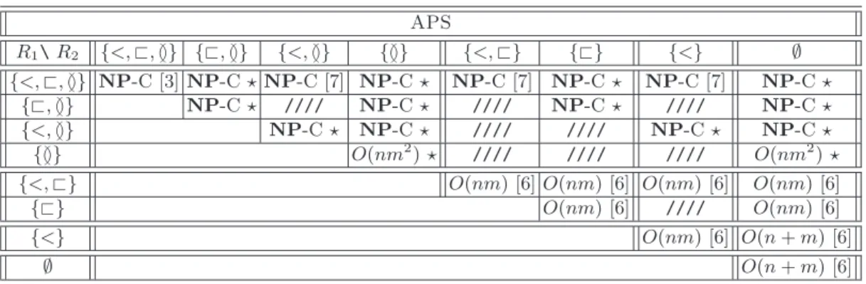
Conversely, Evans has proved that APS(Crossing,Crossing) is NP-complete [3]. A simple reading shows that her proof is concerned with {<, ⊏, ≬}-arc-annotated sequences, and hence she actually proved that APS({<, ⊏, ≬}, {<, ⊏, ≬}) is NP-complete. Similarly, in proving that APS(Crossing,Chain) is NP-complete [7], Guo actually proved that APS({<, ⊏, ≬}, {<}) is NP-complete. Note that according to Observation 1, this latter result implies that APS({<, ⊏, ≬ }, {<, ⊏}) and APS({<, ⊏, ≬},{<, ≬}) are NP-complete. Table 1 surveys known and new results for various types of our refined APS problem. Observe that this paper answers all questions concerning APS problem with respect to both classical and new complexity levels.
APS R1\R2 {<, ⊏, ≬} {⊏, ≬} {<, ≬} {≬} {<, ⊏} {⊏} {<} ∅ {<, ⊏, ≬} NP-C [3] NP-C ⋆ NP-C [7] NP-C ⋆ NP-C [7] NP-C ⋆ NP-C [7] NP-C ⋆ {⊏, ≬} NP-C ⋆ //// NP-C ⋆ //// NP-C ⋆ //// NP-C ⋆ {<, ≬} NP-C ⋆ NP-C ⋆ //// //// NP-C ⋆ NP-C ⋆ {≬} O(nm2 ) ⋆ //// //// //// O(nm2 ) ⋆ {<, ⊏} O(nm) [6] O(nm) [6] O(nm) [6] O(nm) [6]
{⊏} O(nm) [6] //// O(nm) [6]
{<} O(nm) [6] O(n + m) [6]
∅ O(n + m) [6]
Table 1.Complexity results after complexity levels refinement. ////: useless cases. ⋆: results from this paper.
4
Hardness results
We show in this section that APS({⊏, ≬}, ∅) is NP-complete thereby proving that APS(Crossing, Plain) is NP-complete. That result answers an open problem posed by Gramm, Guo and Nieder-meier in [6] which is the last open problem concerning the APS computational complexity with respect to classical complexity levels, i.e., Plain, Chain, Nested and Crossing.
We provide a polynomial time reduction from the well known NP-complete 3-Sat problem [4]: Given a set Vn of n variables and a set Cq of q clauses (each composed of three literals) over Vn, the problem asks to find a truth assignment for Vn that satisfies all clauses of Cq.
It is easily seen that APS({⊏, ≬}, ∅) is in NP. The remainder of the section is devoted to proving that it is also NP-hard. Let Vn = {x1, x2, ...xn} be a finite set of n variables and Cq = {c1, c2, . . . , cq} a collection of q clauses. Observe that there is no loss of generality in assuming that literals are left-right ordered, i.e., if ci= (xj∨ xk∨ xl) then j < k < l. Let us first detail the construction of sequences S and T :
S = Sxs1A S s x1 S s x2A S s x2. . . S s xnA S s xn Sc1 Sc2. . . Scq S e x1 S e x2. . . S e xn T = Ts x1 T s x2. . . T s xn Tc1 Tc2. . . Tcq T e x1 T e x2. . . T e xn
We now detail subsequences composing S and T . Let γm (resp. γm) be the number of oc-currences of literal xm (resp. xm) in Cq. For each variable xm ∈ Vn, 1 ≤ m ≤ n, we con-struct words Ss xm = AC km, Ss xm = C kmA and Ts xm = AC
kmA where Ckm represents a word
of km= max(γm, γm) consecutive bases C. For each clause ci of Cq, 1 ≤ i ≤ q, we construct words Sci = U GGGA and Tci = U GA. Finally, for each variable xm ∈ Vn, 1 ≤ m ≤ n, we construct
words Se
xm = U U A and T
e
xm = U A.
Having disposed of the two sequences, we now turn to defining the corresponding two arc structures (see Figure 1). In the following, Seq[i] will denote the ithbase of a sequence Seq and, for any 1 ≤ m ≤ n, lm= |Ss
xm|. For all 1 ≤ m ≤ n, we create the two following arcs: (S
s xm[1],S e xm[1]) and (Ss xm[lm],S e
xm[2]). For each clause ci of Cq, 1 ≤ i ≤ q, and for each 1 ≤ m ≤ n, if the k
(i.e. 1st, 2ndor 3rd) literal of ci is xm(resp. xm) then we create an arc between any free (i.e. not already incident to an arc) base C of Ss
xm (resp. S
s
xm) and the k
th base G of Sc
i (note that this
is possible by definition of Ss xm, S
s
xm and Sci). On the whole, the instance we have constructed
is composed of 3q + 2n arcs. We denote by APS-cp-construction any construction of this type. In the following, we will distinguish arcs between bases A and U , denoted by AU -arcs, from arcs between bases C and G, denoted by CG-arcs. An illustration of an APS-cp-construction is given in Figure 1. Clearly, our construction can be carried out in polynomial time. Moreover, the result of such a construction is indeed an instance of APS({⊏, ≬}, ∅), since Q = ∅ (no arc is added to T ) and P is a {⊏, ≬}-comparable set (since there are no arcs {<}-comparable).
Lemma 1. Let (S, P ) and (T, Q) be any two arc-annotated sequences obtained from an APS-cp-construction. If (T, Q) can be obtained from (S, P ) by deleting some of its bases together with their incident arcs, if any, then for each 1 ≤ i ≤ q and 1 ≤ m ≤ n : (i) Tci is obtained from Sci by
deleting two of its three bases G, (ii) Te
xm is obtained from S
e
xm by deleting one of its two bases
U, (iii) Ts xm is obtained from S s xmAS s xm by deleting either S s xm or S s xm.
Proof. Let (S, P ) and (T, Q) be two arc-annotated sequences resulting from an APS-cp-construction. (i) By construction, the first base U appearing in S (resp. T ) is Sc1[1] (resp. Tc1[1]). Thus, Tc1[1] is obtained from a base U of S at, or after, Sc1[1]. Moreover, the number of bases A appearing
after Sc1[1] in S is equal to the number of bases A appearing after Tc1[1] in T . Therefore, every
base A appearing after Sc1[1] and Tc1[1] must be matched. That is, for each 1 ≤ i ≤ q, Tci[3] is
matched to Sci[5]. In particular, Tcq[3] is matched to Scq[5]. But since there are as many bases U
between Sc1[1] and Scq[5] as there are between Tc1[1] and Tcq[3], any base U in this interval in S
must be matched to any base U in this interval in T ; that is, for any 1 ≤ i ≤ q, Tci[1] is matched
to Sci[1]. Thus, we conclude that for any 1 ≤ i ≤ q, Tci is obtained by deleting two of the three
bases G of Sci.
(ii) By the above argument concerning the bases A appearing after Sc1[1] and Tc1[1], we know that if (T, Q) can be obtained from (S, P ), then Te
xm[2] is matched to S
e
xm[3] for any 1 ≤ m ≤ n.
Thus, for any 1 ≤ m ≤ n, Te
xm is obtained from S e xm, and in particular T e xm[1] is matched to either Se xm[1] or S e xm[2].
(iii) By definition, as there is no arc incident to bases of T , at least one base incident to every arc of P has to be deleted. We just mentioned that Te
xm[1] is matched to either S
e
xm[1] or S
e xm[2]
for any 1 ≤ m ≤ n. Thus, since by construction there is an arc between Se
xm[1] and S s xm[1] (resp. Se xm[2] and S s
xm[lm]), for any 1 ≤ m ≤ n either S
s
xm[1] or S
s
xm[lm] has to be deleted; and all these
arcs connect a base A appearing before Sc1[1] to a base U appearing after Scq[5]. Therefore, for
any 1 ≤ m ≤ n a base A appearing before Sc1[1] in S is deleted. Originally, there are 3n bases A appearing before Sc1[1] in S and 2n appearing before the first base of Tc1[1] in T . Thus, the number of bases A not deleted in S and appearing before Sc1[1] is equal to the number of bases A appearing before Tc1[1] in T . But since, for each 1 ≤ m ≤ n, a base A of either Ss
xm or S
s xm is
deleted, we conclude that for each 1 ≤ m ≤ n, Ts
xm is obtained from S s xmAS s xm, by deleting either Ss xm or S s xm. ⊓⊔
We now turn to proving that our construction is a polynomial time reduction from 3-Sat to APS(Crossing, Plain).
Lemma 2. Let I be an instance of 3-Sat problem with n variables and q clauses, and I′ an instance ((S, P ); (T, Q)) of APS({⊏, ≬}, ∅) obtained by an APS-cp-construction from I. An as-signment of the variables that satisfies the boolean formula of I exists iff T is an Arc-Preserving Subsequence of S.
Proof. (⇒) Suppose we have an assignment AS of the n variables that satisfies the boolean formula of I. By definition, for each clause there is at least one literal that satisfies it. In the following, ji will define, for any 1 ≤ i ≤ q, the smallest index of the literal of ci (i.e. 1, 2 or 3) which, by its assignment, satisfies ci. Let (S, P ) and (T, Q) be two sequences obtained from an APS-cp-construction from I. We look for a set B of bases to delete from S in order to obtain T .
For each variable xm∈ AS with 1 ≤ m ≤ n, we define B as follows: (i) if xm= T rue then B contains each base of Ss
xm and S
e
xm[1], (ii) if xm= F alse then B contains each base of S
s xm and
Se
xm[2], (iii) if ji = 1 then B contains Sci[3] and Sci[4], (iv) if ji = 2 then B contains Sci[2] and
Sci[4], (v) if ji= 3 then B contains Sci[2] and Sci[3].
Since a variable has a unique value (i.e. T rue or F alse), either each base of Ss
xm and S e xm[1] or each base of Ss xm and S e
xm[2] are in B for all 1 ≤ m ≤ n. Thus, B contains at least one base in
S of any AU -arc of P .
For any 1 ≤ i ≤ q, two of the three bases G of Sci are in B. Thus, B contains at least one
base in S of two thirds of CG-arcs of P . Moreover, Sci[ji+ 1] is the base G that is not in B. We
suppose in the following that the jth
i literal of clause ci is xm, with 1 ≤ m ≤ n. Thus, by the way we build the APS-cp-construction, there is an arc between a base C of Ss
xm and Sci[ji+ 1]
in P . By definition, if AS is an assignment of the n variables that satisfies the boolean formula, AS satisfies ci and thus xm= T rue. We mentioned, in the definition of B that if xm= T rue then each base of Ss
xm is in B. Thus, the base C of S
s
xm incident to the CG-arc in P with Sci[ji+ 1] is
in B. A similar result can be found if the jth
i literal of clause ci is xm. Thus, B contains at least one base in S of any CG-arc of P .
If S′is the sequence obtained from S by deleting all the bases of B together with their incident arcs, if any, then there is no arc in S′ (i.e. neither AU -arcs or CG-arcs). By the way we define B, S′ is obtained from S by deleting all the bases of either Ss
xm or S
s
xm, two bases G of Sci and either
Se
xm[1] or S
e
xm[2], for 1 ≤ i ≤ q and 1 ≤ m ≤ n. It is easily seen that sequence S
′ is similar to T . (⇐) Let I be an instance of 3-Sat problem with n variables and q clauses. Let I′ be an instance ((S, P ); (T, Q)) of APS{⊏, ≬}, ∅) obtained by an APS-cp-construction from I such that (T, Q) can be obtained from (S, P ) by deleting some of its bases (i.e. a set of bases B) together with their incident arcs, if any. By Lemma 1, either all bases of Ss
xm or all bases of S
s
xm are in B.
Consequently, for 1 ≤ m ≤ n, we define an assignment AS of the n variables of I as follows: (i) if all bases of Ss
xm are in B then xm= T rue, (ii) if all bases of S
s
xm are in B then xm= F alse.
Now, let us prove that for any 1 ≤ i ≤ q clause ci is satisfied by AS. By Lemma 1, for any 1 ≤ i ≤ q there is a base G of segment Sci (say the ji+ 1
th) that is not in B. By the way we build the APS-cp-construction, there is a CG-arc in P between Sci[ji+ 1] and a base C of S
s xm (resp. Ss xm) if the j th i literal of ci is xm (resp. xm). Suppose, w.l.o.g., that the jth
i literal of ci is xm. Since Q is an empty set, at least one base of any arc of P is in B. Thus, the base C of Ss
xm incident to the CG-arc in P with Sci[ji+ 1] is in
B (since Sci[ji+ 1] 6∈ B). Therefore, by Lemma 1, all the bases of S
s
xm are in B. By the way we
define AS, xm= T rue and thus ci is satisfied. A similar result can be obtained if the jth
i literal of
ci is xm. ⊓⊔
We have thus proved the following.
Theorem 1. APS({⊏, ≬}, ∅) is NP-complete.
It follows immediately from Theorem 1 that APS({<, ⊏, ≬}, ∅), and hence APS(Crossing, Plain), are NP-complete. One might naturally ask for more information concerning hard cases
of APS problem in order to get valuable insight into what makes the problem difficult. Another refinement of the hardness of APS(Crossing,Plain) is given by the following theorem.
Theorem 2. APS({<, ≬}, ∅) is NP-complete.
Proof (Sketch of ). The proof is also by reduction from 3-Sat. Due to space considerations, the rather technical proof is deferred to the full version of the paper and only sketch main ideas behind Theorem 2. One of the reasons making the proof complicated is that all arcs have to be {<, ≬}-comparable, and hence we can not close an arc before closing all arcs which have been opened before. To overcome this problem we need pairs of strings gadgets which act as “signal repeaters” so that we can close and re-open a link carrying a truth value. Actually, repeaters unfortunately invert truth value and hence we need to deal with pairs of repeaters (first kind and second kind repeaters) where each repeater of the second kind is paired with a repeater of the first kind. ⊓⊔
5
Two polynomial time solvable
APS problems
We prove in this section that APS({≬}, ∅) and APS({≬},{≬}) are polynomial time solvable. In other words, relation ≬ alone does not imply NP-completeness. We need the following notations. Sequences are the concatenation of zero or more elements from an alphabet. We use the period “.” as the concatenation operator, but frequently the two operands are simply put side by side. Let T = T [1] T [2] . . . T [m] be a sequence of length m. For all 1 ≤ i ≤ j ≤ m, we write T [i : j] to denote T [i] T [i + 1] . . . T [j]. The reverse of T is the sequence TR = T [m] . . . T [2] T [1]. A factorization of T is any decomposition T = x1x2. . . xq where x1, x2, . . . xq are (possibly empty) sequences. Let (T, A) be a {≬}-arc-annotated sequence and (i, j) ∈ A, i < j, be an arc. We call T [i] a forward base and T [j] a backward base. We will denote by LFT the position of the last forward base in (T, A) and by FBT the position of the first backward base in (T, A), i.e., LFT = max{i : (i, j) ∈ A} and FBT = min{j : (i, j) ∈ A}. By convention, we let LFT = 0 and FBT = |T | + 1 if A = ∅. Observe that LFT < FBT. We begin by proving a factorization result on {≬}-arc-annotated sequences. Lemma 3. Let S and T be two {≬}-arc-annotated sequences of length n and m, respectively. If T occurs as an arc preserving subsequence in S, then there exists a factorization (possibly trivial) T [LFT+1 : FBT−1] = xy such that T [1 : LFT] · x · (y · T [FBT : m])R occurs as an arc preserving subsequence in S[1 : FBS−1] · S[FBS : n]R.
Proof. Suppose that T occurs as an arc preserving subsequence in S. Since both S and T are {≬}-arc-annotated sequences, then there exist two factorizations S[1 : LFS] = uw and S[FBS : n] = zv such that: (i) T [1 : LFT] occurs in u, (ii) T [LFT+1 : FBT−1] occurs in w · S[LFS+1 : FBS−1] · z and (iii) T [FBT : m] occurs in v. Then it follows that there exists a factorization T [LFT+1 : FBT−1] = xy such that x occurs in w · S[LFS+1 : FBS−1] and y occurs in z, and hence T′ = T [1 : LFT] · x · (y · T [FBT : m])R occurs as an arc preserving subsequence in S′= S[1 : FBS−1] · S[FBS: n]R ⊓⊔ Theorem 3. APS({≬},{≬}) is solvable in O(nm2
) time. Proof. The algorithm is as follows:
Data : Two {≬}-arc-annotated sequences S and T of length n and m, respectively Result: true iff T occurs as an arc-preserving subsequence in S
begin
1 S′= S[1 : FBS−1] · S[FBS: n]R
2 foreachfactorization T [LFT+1 : FBT−1]| = xy do 3 T′= T [1 : LFT] · x · (y · T [FBT: m])R
4 if T′ occurs as an arc preserving subsequence in S′then 5 return true
6 return false end
Correctness of the algorithm follows from Lemma 3. What is left is to prove the time complexity. Clearly, S′ = S[1 : FBS−1] · S[FBS : n]R is a {⊏}-arc-annotated sequence. The key point is to note that, for any factorization T [LFT+1 : FBT−1]| = xy, the obtained T′ = T [1 : LFT] · x · (y · T [FBT : m])R is a {⊏}-arc-annotated sequence as-well. Now let k be the number of arcs in T . So there are at most m − 2k iterations to go before eventually returning false. According to the above, Line 4 constitutes an instance of APS({⊏},{⊏}). But APS({⊏},{⊏}) is a special case of APS({<, ⊏},{<, ⊏}), and hence is solvable in O(nm) time [6]. Then it follows that the algorithm as a whole runs in O(nm(m − 2k)) = O(nm2
) time. ⊓⊔
Clearly, the proof of Theorem 3 relies on an efficient algorithm for solving APS({⊏},{⊏}): the better the complexity for APS({⊏},{⊏}), the better the complexity for APS({≬},{≬}). We have used only the fact that APS({⊏},{⊏}) is a special case of APS({<, ⊏},{<, ⊏}). It remains open, however, wether a better complexity can be achieved for APS({⊏},{⊏}). Theorem 3, combined with Observation 1, carries out easily to restricted versions.
Corollary 1. APS({≬},∅) is solvable in O(nm2 ) time.
6
Conclusion
In this paper, we investigated the APS problem time complexity and gave a precise charac-terization of what makes the APS problem hard. We proved that APS(Crossing,Plain) is NP-complete thereby answering an open problem posed in [6]. Note that this result answers the last open problem concerning APS computational complexity with respect to classical complexity levels, i.e., Plain, Chain, Nested and Crossing. Also, we refined the four above mentioned levels for exploring the border between polynomial time solvable and NP-complete problems. We proved that both APS({⊏, ≬}, ∅) and APS({<, ≬}, ∅) are NP-complete and gave positive results by showing that APS({≬}, ∅) and APS({≬},{≬}) are polynomial time solvable. Hence, the refine-ment we suggest shows that APS problem becomes hard when one considers sequences containing {≬, α}-comparable arcs with α 6= ∅. Therefore, crossing arcs alone do not imply APS hardness. It is of course a challenging problem to further explore the complexity of the APS problem, and especially the parameterized views, by considering additional parameters such as the cutwidth or the depth of the arc structures.
References
1. J. Alber, J. Gramm, J. Guo, and R. Niedermeier. Computing the similarity of two sequences with nested arc annotations. Theoretical Computer Science, 312(2-3):337–358, 2004.
2. G. Caetano-Anoll´es. Tracing the evolution of RNA structure in ribosomes. Nucl. Acids. Res., 30:2575– 2587, 2002.
3. P. Evans. Algorithms and Complexity for Annotated Sequence Analysis. PhD thesis, U. Victoria, 1999. 4. M. Garey and D. Johnson. Computers and Intractability: A Guide to the Theory of NP-Completeness.
W. H. Freeman and Company, 1979.
5. D. Goldman, S. Istrail, and C.H. Papadimitriou. Algorithmic aspects of protein structure similarity. In Proc. of the 40th Symposium of Foundations of Computer Science (FOCS99), pages 512–522, 1999. 6. J. Gramm, J. Guo, and R. Niedermeier. Pattern matching for arc-annotated sequences. In Proc. of the 22nd Conference on Foundations of Software Technology and Theoretical Computer Science (FSTTCS02), volume 2556 of LNCS, pages 182–193, 2002.
7. J. Guo. Exact algorithms for the longest common subsequence problem for arc-annotated sequences. Master’s Thesis, Universitat Tubingen, Fed. Rep. of Germany, 2002.
8. T. Jiang, G.-H. Lin, B. Ma, and K. Zhang. The longest common subsequence problem for arc-annotated sequences. In Proc. 11th Symposium on Combinatorial Pattern Matching (CPM00), volume 1848 of LNCS, pages 154–165. Springer-Verlag, 2000.
9. V. Juan, C. Crain, and S. Wilson. Evidence for evolutionarily conserved secondary structure in the H19 tumor suppressor RNA. Nucl. Acids. Res., 28:1221–1227, 2000.
10. G. Lancia, R. Carr, B. Walenz, and S. Istrail. 101 optimal PDB structure alignments: a branch-and-cut algorithm for the maximum contact map overlap problem. In Proceedings of the 5th ACM International Conference on Computational Molecular Biology (RECOMB01), pages 193–202, 2001.
11. S. Vialette. On the computational complexity of 2-interval pattern matching. Theoretical Computer Science, 312(2-3):223–249, 2004.
12. K. Zhang, L. Wang, and B. Ma. Computing the similarity between RNA structures. In Proc. 10th Symposium on Combinatorial Pattern Matching (CPM99), volume 1645 of LNCS, pages 281–293. Springer-Verlag, 1999.