HAL Id: dumas-00725335
https://dumas.ccsd.cnrs.fr/dumas-00725335
Submitted on 24 Aug 2012
HAL is a multi-disciplinary open access
archive for the deposit and dissemination of
sci-entific research documents, whether they are
pub-lished or not. The documents may come from
L’archive ouverte pluridisciplinaire HAL, est
destinée au dépôt et à la diffusion de documents
scientifiques de niveau recherche, publiés ou non,
émanant des établissements d’enseignement et de
Privacy implications of geosocial proximity
Antoine Rault
To cite this version:
Antoine Rault. Privacy implications of geosocial proximity. Distributed, Parallel, and Cluster
Com-puting [cs.DC]. 2012. �dumas-00725335�
Privacy implications of geosocial proximity
Antoine RAULT
supervised by S´
ebastien Gambs and Olivier Heen
Abstract
Geosocial networks, social networks integrating their users’ location, meet an undeniable success. While traditional social networks are already subject to privacy breaches, the addition of location make such breaches to pile up. However, a not obvious question is : does this combination create a new type breaches which were not previously conceivable by the sole use of social networks or location information? We address this matter in two experiments. A first one which takes geosocial network users’ profiles and classify them depending on whether their friends live globally close to or far from them. We find that 70 % of users in our Foursquare dataset have their friends living relatively close to them. The second experiment that we led use the check-ins of Gowalla and Brightkite users to discover their social graphs. The check-ins model the users’ movements then we assume that users whose modellings are sufficiently similar are friends. This assumption comes from the fact that one often makes new friends in the places that he likes and where he spends a long time. Our partial findings seems to indicate that we are able to discover a half of a user’s social graph in average. Thus, we attempt a beginning of answer saying that geosocial networks actually allow new types of attacks against their users’ privacy.
Keywords : Privacy, Geosocial Networks, Geographic Proximity, Link Prediction, Check-ins, Similarity Measure.
R´esum´e
Les r´eseaux sociaux g´eolocalis´es, des r´eseaux sociaux int´egrant la lo-calisation de leurs utilisateurs, rencontrent un succ`es ind´eniable. Alors que les r´eseaux sociaux traditionnels sont d´ej`a sujets `a des br`eches de la vie priv´ee, l’ajout de la localisation fait s’empiler de telles br`eches. Cepen-dant, une question non-´evidente est : est-ce que cette combinaison cr´ee de nouveaux types de br`eches qui n’´etaient pas envisageables pr´ec´edemment par le seul usage des r´eseaux sociaux ou des information de localisation ? Nous traitons ce sujet dans deux exp´eriences. Une premi`ere qui prend les profiles des utilisateurs des r´eseaux sociaux g´eolocalis´es et les classe selon que leurs amis vivent globalement pr`es ou loin d’eux. Nous trouvons que 70 % des utilisateurs dans notre jeu de donn´ees de Foursquare ont leurs amis qui vivent relativement pr`es. La seconde exp´erience que nous avons men´e utilise les “check-ins” des utilisateurs de Gowalla et Brightkite
afin de d´ecouvrir leurs graphes sociaux. Les “check-ins” mod´elisent les mouvements des utilisateurs et nous supposons que des utilisateurs dont les mod´elisations sont suffisamment similaires sont amis. Nous faisons cette supposition en nous basant sur le fait qu’on se fait souvent de nou-veaux amis dans les lieux que l’on aime et o`u l’on passe un long mo-ment. Nos d´ecouvertes partielles semblent indiquer que nous sommes ca-pables en moyenne de d´ecouvrir la moiti´e du graphe social d’un utilisateur. Ainsi, nous tentons un d´ebut de r´eponse disant que les r´eseaux sociaux g´eolocalis´es permettent en fait de nouveaux types d’attaques contre la vie priv´ee de leurs utilisateurs.
Contents
1 Introduction 3 1.1 Geosocial networks . . . 3 1.2 Privacy issues . . . 4 1.3 Introductory work . . . 7 1.4 Terminology . . . 8 1.4.1 Models of adversary . . . 8 2 Related Work 9 3 Geographic distance of one’s friends 10 3.1 Foursquare dataset . . . 103.2 Application to the Foursquare dataset . . . 12
3.2.1 Results . . . 12
3.2.2 Average distance of friends algorithm . . . 14
3.3 Implications . . . 16
4 Predict one’s social graph based on location 16 4.1 Gowalla and Brightkite datasets . . . 17
4.2 Inferring social graph through geographic proximity . . . 18
4.3 Application to the Gowalla and Brightkite datasets . . . 20
4.3.1 Results . . . 20
4.4 Complexity and computation time . . . 21
5 Conclusion 22 5.1 Discussion on the results . . . 22
5.2 Possible future work . . . 23
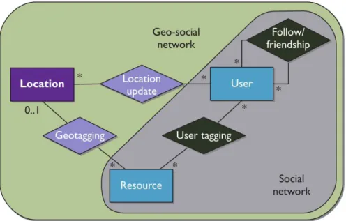
Figure 1: Logical representation of a geosocial network
1
Introduction
1.1
Geosocial networks
Geolocated social networks (abbreviated geosocial networks) follow the same approach as traditional social networks but add location information to the range of publishable contents. In order to understand how geosocial networks function, one must know how standard ones work. Social networks [BE07] are websites in which users create themselves an identity, then link it to other people’s identities (often, yet not always, people they know in real life), thus defining a kind of relationship with those people. Once this is done, the new user can share content. The content can be made public or selectively shared with a subset of his contacts, depending on the relationship with them for instance. Most commonly shared contents include texts (thoughts, actions, reviews, chats, etc.), reactions to the content someone shared with you, pictures, music, videos, web links or even invitations to participate in a game. Even if the majority of social networks feature the previously described mechanisms, not all of them work the same way because they differ in their purpose. Some are general-purposed, like Facebook or Google+, while some focus on specific goals such as finding out what former classmates have become like Copainsdavant [Gro] or recreating one’s business network of contacts like LinkedIn.
Geosocial networks offer location as an additional type of content as well as a geo-tagging mechanism, which is the possibility to associate geographical information to a content. Using this mechanism, one can publish its current
location or geolocate the place in which a photo has been taken, as illustrated with Fig 1. Moreover, geosocial networks also feature access through a mobile application because the advent of smartphones embedding a GPS chip allows one to share geolocated content in a simple way, at any time. Similarly to tra-ditional social networks, their geolocated counterparts target various markets. For instance, the main types of geosocial networks are :
• A classic social network adding a feature mimicking some geosocial net-work paradigm. The addition can be passive continuous location or active momentary location. Example : Facebook Places (discontinued since Au-gust 2011).
• Users actively check-in at places of interest. It means that they publish their location when they go to a place defined in the geosocial network (often bars, restaurants, shops, etc.). These check-ins are shared with the user’s friends so they may know he is at this given location. Additionally, checking-in makes users earn virtual or actual rewards. If one checks-in regularly at the same places or, on the contrary, at many new places, he will earn virtual achievement certificates showing to his friends his actions. If the places where one checks-in sell something, he may get some exclusive discount or invitation. Example : Foursquare.
• Users write reviews places of interest. These reviews are public but a social networking site allows users to share reviews, communicate privately and keep track of reviews friends wrote, liked or reacted to. Since reviews can be evaluated by other users, making good reviews earns them reputation points. Example : Qype [Gmb].
• A blogging service whose posts are geolocated. Like any micro-blogging service, messages published by users are public and have a voca-tion of instantaneous informavoca-tion exchange. Social networking is realized through asymmetric relations of subscription to one’s posts and private messaging is enabled when two users have subscribed to each other. Ex-ample : Twitter.
1.2
Privacy issues
While traditional social networks are already an important source of privacy breaches, the geosocial networks pose an even bigger threat to privacy because they might leak location of their users. Indeed, one’s past, present or future location being among the most personal information, you would not want it to be available to anyone among your acquaintances or even more to someone outside of the geosocial network.
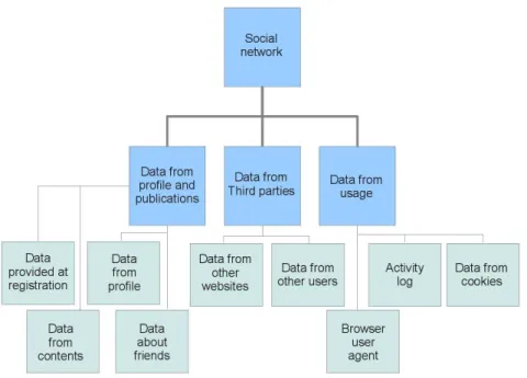
First of all, when covering problems of privacy in geosocial networks, one must consider sources of the information about its users that a network uses. It is not directly a privacy issue but the fact that users are not aware of everything the network knows favours less careful behaviours. Obviously, the main source
Figure 2: The sources of information for geosocial networks
of information is the data of users’ profile itself (information given when signing up, content published, etc.) and users are aware of this. Another source is made of the way the network is used : when do users connect themselves? Do they use it via a web browser or smartphone? Etc. Most of the users are not aware that the geosocial network deduces new knowledge about its users from their usage. Finally, the network learns about its users because of the information provided by third parties. Examples of such third parties are other users of the network or other websites the network’s users are member of. Suppose Alice and Bob are friends on a geosocial network. Bob uploads a geo-tagged photo of a party in which Alice is visible. Later, Charlie, a friend of Bob, puts a tag on the photo uploaded by Bob saying that Alice is present on it. Now, the network knows that Alice went at the party and that Charlie and her know each other, even if she did not want these information to be present in the network. This becomes problematic since anything known by the network is not safe from a security breach.
Moreover, even if they do not suffer from security breaches, geosocial net-works are subjects to several types of privacy issues [VFBJ11].
• The first one concerns location privacy, which is about disclosing one’s exact location. Users do not always want nor need to publish their precise location, all the more if anyone can access it. Despite, the ability offered by some services like Twitter to provide a coarser location than what
is actually available, users’ exact location can still be revealed through other users’ publications. Suppose that for instance, Alice publishes “Just arrived in Ireland for holidays” to all her friends, then Alice’s friend, Bob who lives in Dublin writes “I am at the airport to pick up Alice”. Half an hour later, Charlie, another friend of Alice, says “Fine Japanese meal at the restaurant with Alice and Bob”. In spite of Alice, Bob and Charlie’s efforts to keep their location secret, a mutual friend of them is able to determine that they are in a Japanese restaurant located near Dublin’s airport.
• Absence privacy issues are about knowing that someone is not some-where at a given moment. It sometimes happens when one disclose a current location different from the one he is supposed to be, thus allowing another to discover a lie. Suppose that for example, Bob tells his mother Alice that he will be working his exams at in his room for the whole after-noon. But if Alice sees an update at 4 p.m. from Bob saying “Charlie’s pool is so refreshing”, she will know that he is not in his room any more. • Co-location privacy issues refer to problems where the presence of sev-eral people in the same place, at the same time is to be kept secret. For example, Alice, Bob and Charlie are very good friends who always go out together. For Charlie’s birthday, Alice and Bob want to buy him some martial art kit as a present. It is okay if only Alice posts a message saying “I am at the Budo Shop”, but if Bob’s friend Erica publishes within min-utes “Just met Bob at the Budo Shop, I did not know he was into martial arts”, Charlie might start to be suspicious.
• An identity privacy issue means that unlinkability [PDH08] between one’s real identity and pseudonym is not assured. While using a pseudonym in social networking services might sometimes be enough to prevent some-one from linking it to a real person, the addition of geolocation can no-ticeably reduce the efficiency of such a method. For instance, Bob is using an online geolocated dating service under the pseudonym Charlie and ob-viously do not want his wife Alice to know it. One evening, he tells her that he will stay at work late. If Alice logs herself into the dating service the same evening, she will sees that the only user of this service located at Bob’s work place is Charlie. She will be able to deduce that Charlie is highly likely to be Bob.
• Lastly, it is common for geosocial networks or carriers selling smartphones to release mobility datasets for research of industrial purposes1
. Of course, these sets are sanitized before being made public by anonymizing mobil-ity traces and applying spatial or temporal cloaking for example [GG03]. However, these techniques are not always sufficient to prevent attackers
1
CRAWDAD, which stands for Community Resource for Archiving Wireless Data At Dartmouth, (crawdad.cs.dartmouth.edu) and the North American Open Geocode (open-geocode.org) are examples of public repositories of geolocated data.
to learn information on users whose mobility traces are found in public sets [GKdPC10]. Using inference attacks, one can discover users’ places of interest (PoI) such as the location of his home, the company he works for, the places where he practices sports and leisures, his usual itineraries, etc. When an attacker knows these kind of PoI, he has the possibility to predict someone’s past, present and future location. If the prediction pro-cess is reliable enough, it can be envisioned to use it to detect if someone is lying about its location. Inference attacks also allow to de-anonymize datasets [SG12]. Once a signature characterising a mobility trace has been generated, it may be used to detect the presence of the same people in other datasets.
All these privacy issues originate from three facts. Some problems are caused because the website used is a social network. An example of inherent risk in social networks is that a user’s boss learns he thinks of him as a stupid person because the network changed its default privacy settings. Some other prob-lems come from the fact that the service used is geolocated. For instance, an excessively jealous women can surreptitiously make her husband’s smartphone subscribe to a continuous location service so that she can track him. Finally, some issues happen because the service used by someone has features of geolo-cation as well as of social networking. It means that some privacy breaches exist only when these two types of features are associated. Suppose that a user of a geosocial network tells his wife that he will be working late and during the evening, he checks-in at a pub. We have a privacy breach here because the user’s wife will discover that her husband lied. If the service was not geolocated, there would not be such a problem. If the service was not social but public instead, the user would have likely be more careful about its uploaded locations so there would not be a breach either.
1.3
Introductory work
• In [BE07], Danah M. Boyd and Nicole Ellison provide a definition of social networks and survey the academic research field social networks. This a good base to have when addressing such a subject as geosocial networks. • In [PDH08], Andreas Pfitzmann and Marit Hansen define precisely and abundantly several terms relating to privacy such as anonymity, unlink-ability or pseudonymity. It is useful so that everyone in the community give the same meaning to these words.
• In [Pot11], Christophe Potin reports his work on analysing security and privacy of geosocial networks. Our work is the follow-up of his one. More-over, we use datasets collected by Christophe Potin in section 3.
• In [VFBJ11], Carmen Ruiz Vicente, Dario Freni, Claudio Bettini and Christian S. Jensen define 4 types of attacks on privacy in geosocial net-works as well as means of protection against each of them. Their
defini-tions are excellent and clear. By the way, we used them extensively as inspiration to define the privacy issues in the previous section.
1.4
Terminology
Let us define precisely some terms that we use, to avoid any possible confusion. Definition. A geosocial network user is an individual who is member of a geosocial network. Generally, a user is ??? by identification number. We use only “user” to designate those individuals from here.
Definition. A social graph is a graph representing social relationships. Nodes are users and edges are social links such as friendship. Specifically, we often talk about a user’s social graph.
Definition. A friend of a user designates a member of that user’s social graph. Thus, all the friends of a user in the social graph are not necessarily considered by him as friends in the usual way. He may actually consider some or all of them as merely acquaintances in real life. The relation is mutual in Facebook, and Gowalla and not mutual in Brightkite, and Twitter, for instance.
Definition. The main location of a user is the location that he advertises as the place where he belongs. This location usually is his hometown.
Definition. A target user is a user concerned by our experiments. It means that he is the user of which we compute the global proximity of his friends or for who we predict friends.
Definition. A place of interest is a place where people would want to go and record their presence there. We use the abbreviated version, PoI.
Definition. A check-in is the timestamped location of a user. Users may check-in at places of interest and share it with their friends.
Definition. A check-in class is a set of all the check-ins made by any user at the same place.
Definition. The geodesic distance between two points is the length of the curve between two points on a mathematical model of the Earth. The points as well as the curve linking them are on the surface of the modelled Earth. We use it to find an approximation of the actual distance as the crow flies that one must cover to get from one point designated by GPS coordinates to another.
1.4.1 Models of adversary
An adversary may run an attack against a geosocial network to create a breach of its users’ privacy. If the adversary succeeds, it gathers private personal in-formation for malicious purposes. In our context, we distinguish between three categories of adversary :
• Geosocial network operator : Taking advantage of his extended priv-ileges in the system, he might access any piece of information that the user provided to the geosocial network. This makes him the most difficult type of adversary to protect from. The operator himself may be malicious and willingly attack the users’ privacy or, more likely, someone else could hijack his account in the system and act in his name. Often, he is a pas-sive adversary, that is to say he tries to extract as much information as possible rather than to alter the user’s data. This type of adversary is used in our experiment from section 3.
• User : Usually, he has access to more information than a third party adversary, regarding other users, including those which are not part of his social graph. If an adversary user wants more information than the default subset available to non-friends of a given user, he may use social engineering. Indeed, he may prepare his attack with a social engineering phase intended to introduce himself in the target’s social graph.
• Third party : This entity is totally external to the geosocial network. Accordingly, it has no privileges and only has access to two types of infor-mation. They are information either made public by the users or revealed by observing the system, e.g. URLs, cookies, traces in search engines, etc. We user this adversary in our experiment from section 4.
In this work, when we take on a defencive role, we do not account for col-lusions of many adversaries trying to infiltrate the network. When we take on the offencive role of an adversary, we assume that all user provided information is genuine, especially location-related information. These problems are out of our scope and would require dedicated work for each of them. Finally, in either role, we consider only information published directly by users about themselves. Situations when information concerning a user is revealed by others cannot be addressed in most cases, so we do not mention them.
2
Related Work
• In [ZG09], Elena Zheleva and Lise Getoor show how privacy is an illusion as soon as friends can have public profiles and membership in groups of interest are public. We use a similar type of reasoning as, in geosocial networks, one’s non-public location can be deduced from his friends’ public location.
• In [BSM10], Backstrom, Sun and Marlow expose an algorithm predicting the location of Facebook users by using their friends’ location and using IP-based location when there is not enough friends. This paper is very similar in its idea as our experiment in section 3
• [SNM11] is a similar work in which Cambridge’s researchers use check-in data of a user to predict which users he is likely to become friend with.
• In [LCB10], Vincent Leroy, B. Barla Cambazoglu and Francesco Bonchi develop an algorithm requiring no initial knowledge of a user’s social graph to recover it. They use instead membership of groups of interest. We use the same idea of no requirement knowledge of the user’s social graph in section 4
3
Geographic distance of one’s friends
We address the question of whether typical user’s friends generally live close to him or far from him? We researched this issue because we wanted to point out simple correlations between the social data and the geographic data in a geosocial network.
This experiment relies on datasets made of users’ profiles from the Foursquare geosocial network. As a third party adversary would do, we gather the main location of target users and their friends, from their public profiles. Then we geocode these locations. It allows us to compute the geodesic distance between the target users and each of their friends. Finally, we calculate the average value of each target user’s set of distances. Thus, we can classify target users as hav-ing friends near or far from them, dependhav-ing on whether the average distance is respectively below or above a threshold distance.
We find that the average distance of a target user’s friends is 1,648 km, which is relatively close when considering the United States of America where 50% of Foursquare’s users reside [Tso]. Using a threshold distance of 1,648 km, 70% of users fall into the “close friends” category. We show that, 24,6% of users have at least a half of their friends living within the same city. We also observe that users with many friends tend to have more geographically scattered friends than users with few friends.
3.1
Foursquare dataset
In this subsection, we describe the dataset used to conduct our experiment. We had three datasets at our disposal, originating from three different geosocial networks. This was made possible thanks to Christophe Potin’s internship, supervised by S´ebastien Gambs and Olivier Heen as well, on privacy in geosocial networks [Pot11]. He crawled and retrieved data from Foursquare, Justacot´e and La Ruche.
However, we do not consider the Justacot´e and La Ruche datasets because we did not deem them meaningful enough. Concerning the Justacot´e dataset, we actually ran our experiment over it but we only got the average distance of friends (1266 km in average) for 5 target users out of the 1587 ones avail-able. Moreover, 4 of the resulting average distances were computed using only 1 friend’s main location. As for the dataset from La Ruche, we do not use it because there is no explicit friendship link, thus making our experiment in-applicable. However, it is worth noting that this dataset could become useful after rebuilding users’ social graph thanks to the bootstrap probabilistic graph
method [LCB10]. Such social graph prediction is possible because of the users’ profiles tags. Indeed, users may associate tags such as “Art”, “Bier” or “Fest-Noz” with their profile to represent their centres of interest. These tags are almost identical to Flickr’s groups of interest used in [LCB10].
Foursquare is an American geosocial network and the largest one with 20,000,000+ members. It enables its users to check-in at places of interest and share it with their friends. The more users check-in, the more badges (virtual symbols of achievement) and actual rewards (discounts, special offers, etc. in the commer-cial establishments they checked-in at) they earn.
The dataset was collected using a Python script written by Christophe Potin specifically for this purpose. It made all its connections to Foursquare’s website through the Tor network, a system that provides anonymity and protects its users’ privacy. Tor was used to avoid turning the attention of the network’s op-erators to its data collection. Moreover, the programme waited a random period of time between 10 and 30 seconds, before loading each webpage. This was done with the same goal in mind as previously and to avoid overloading Foursquare as well. The webpages which the script aimed at as starting points for collection were users’ profiles. They were selected randomly and their number depended on the total number of users. Once these users’ profiles have been collected, the profile of their friends that were accessible from it were also collected. A direct access to user’s profile is possible without a priori knowledge, such as users’ pseudonym, because Foursquare use enumerable identifiers for its users. Each user is identified by a unique number assigned to him. This number is chosen as the value of a counter which is incremented of one at each successful user registration. This allows to guess the url of a user’s profile. In Foursquare, profiles’ urls are structured as foursquare.com/user/<userID>/.
Finally, here are additional characteristics of the Foursquare dataset : • Total current number of users : 20,000,000+
• Total number of users at the time of collection : 10,000,000+ • Number of users’ profile collected : 23,705
• The maximum number of friends’ profiles retrieved from a given user’s profile is 10 because it is the size of the sample of friends shown when the user has more than 10 friends. This sample is randomly composed among all of a user’s friends each time his profile is accessed. However, it is useless to reload several times the same profile as the algorithm generating the sample makes sure that the number of newfound friends is quickly decreasing until no more new friends are shown.
• A tiny fraction of users’ profiles do not represent an individual but rather a brand or a company. A main location cannot be provided for these profiles (its meaning would be different anyway) thus making them irrelevant for our purpose. We detect and eliminate these profiles because they do not contain the HTML tags surrounding the main location string usually found in individuals’ profiles.
• The webpage listing all the badges earned by a user has been collected for each user who was a starting point of collection.
3.2
Application to the Foursquare dataset
3.2.1 Results
Among the 20,000+ profiles in the dataset, we use 7,885 of them as target users. Only profiles meeting several criteria are eligible to be used as target user. They must be a starting point of collection, belong to an individual and mention his main location. Identifiers of the target users range from 576 to 11693489 (users with lower IDs registered first).
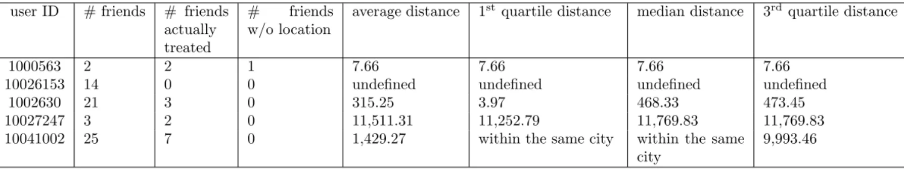
Table 1 is an excerpt of the raw results of our experiment. There is two special values in columns supposed to contain distances. “undefined” is used when the dataset do not contain any profile of the target user’s friends. “within the same city” is used when the geodesic distance is 0.0 km because a null distance between two users does not make sense. It means that the target user and some of his friends indicated more or less the same main location string. We choose the word “city” because it is the most common granularity of main location on profiles. Attention, any non-null distance does not appear as “within the same city”, even if it is very small. It means that users may be living in the same city even if this special value is not used.
Table 2 presents some notable figures. We see that Foursquare’s users have few friends for a social network, with a mean number of almost 9. For example, an average user of Facebook had 190 friends in May 2011 [UKBM11]. Even if Facebook is much bigger (721 millions of users then, 901 millions now), the total number of users/mean number of friends ratio of Foursquare is smaller. We can partially explain this by their difference of age. The geosocial network launched in 2009 while the traditional social network launched in 2004.
We also observe that almost all users provide their main location as only 1.1% of the 12,136 friends profiles lack this piece of information. It is not surprising given the focus of Foursquare on geolocation. However, we find that more than 40% of users in our dataset have no friends. This is not an usual
user ID # friends # friends actually treated
# friends w/o location
average distance 1st
quartile distance median distance 3rd
quartile distance
1000563 2 2 1 7.66 7.66 7.66 7.66
10026153 14 0 0 undefined undefined undefined undefined 1002630 21 3 0 315.25 3.97 468.33 473.45 10027247 3 2 0 11,511.31 11,252.79 11,769.83 11,769.83 10041002 25 7 0 1,429.27 within the same city within the same
city
9,993.46
Highest # friends 989 (user 2946815) Average # friends / target user 8.88
Highest average distance 16,326.71 km (user 4038406) # friends w/o location 134 (1.1% of friends’ profiles) Average # friends w/o location / target user 0.14
# target users w/o friends 3,306 (41.9% of target users) Table 2: Notable figures from our results
# target users 910 (11.5%) Average # friends / target user 32.32 Average # exploitable friends / target user 6.51
Highest average distance 16,196.81 (user 1244117) Average distance of friends 1,648.23
# target users w/ average distance within same city 34 (3.7%) # target users w/ 1st
quartile distance within same city 399 (43.8%) # target users w/ 3rd
quartile distance within same city 244 (24.6%)
Table 3: Interesting figures using our significant results only (unit of distance : kilometre)
number for such a website. Its interest is drastically reduced if one do not share his check-ins.
This leads us to address the subject of significance of some target users. Obviously, target users having no friends are useless to us. We also consider as insignificant those for who we do not have at least 5 exploitable friends’ profiles. We set the significance threshold to 5 because in [BSM10], Backtrom et al. show that their main location prediction through friends locations algorithm performs efficiently enough with as low as 5 friends.
We now look at our results when limiting ourselves with significant target users. Table 3 gathers some interesting results. We immediately note that our dataset contains just a little more than 10% of significant target users. It is a relatively low percentage of useful data. We could conclude that the data col-lection method is bad but we must also keep in mind that this dataset was not initially collected for the same goal as our experiment. Particularly interesting is the global the average distance of friends that we find to be 1,648 km. We say that this is a relatively close distance because in mid-2011, 50% of Foursquare’s users lived in the United States of America. The USA being one of the four biggest country in terms of area, we expect a greater average distance of friends for USA’s inhabitants. It seems to be false because the important proportion of Americans must impact significantly the global average distance of friends. We suppose that this proportion is the same in our dataset because the data was collected sometime between late-March and mid-August of 2011, and because target users were chosen randomly, thus following a uniform distribution. Fi-nally, we observe that even though users rarely have their friends globally living
many (100+) friends few (5 to 10) friends # target users 40 (4.3%) 218 (23.9%) Mean average distance 1,873.22 1,749.88 Mean 1st
quartile distance 507.55 1,045.37 Mean 3rd
quartile distance 5,094.74 3,850.04
Table 4: Interesting figures about users having many or few friends (unit of distance : kilometre)
close friends far away friends # target users 636 (69.9%) 274 (30.1%) Mean # friends / target user 29,95 37,80 Mean average distance 449.04 4,431.76 Mean 1st
quartile distance 94.15 2,239.19
Table 5: Notable results about users having their friends living close to or far from them (unit of distance : kilometre)
in the same city (3,7%), an important part of them has at least a quarter of their friends in the same city (43,8%).
In table 4, we look at various results regarding target users with few/many friends. We find that users with many friends (100+) and those with few friends (up to 10) have a similar average distance of their friends. This average distance is of approximately 1,800 km. However, we see that the two types of users differ in the geographic repartition of their friends. Users with many friends tend to have them more scattered. A half of their friends live between 500 km and 5,100 km in average. On the other hand, users who have few friends choose them in a more concentrated area. For instance, 50% of those users’ friends live between 1,000 km and 3,800 km in average.
Finally, table 5 shows notable differences between users whose friends live close to them and users whose friends live far from them. We set the threshold distance to differentiate users to 1,648 km, the global average distance of friends. We see that 70% of users have their friends close to them. We note that users whose friends live far away also have more friends in average. More surprising than the difference in average distances is the difference in 1st
quartile distances of the two categories of users. Indeed, users whose friends live close to them have 25% of their friends living at 21% of their average distance. Regarding users whose friends live far from them, they have 25% of their friends living at 50% of their average distance. It seems to confirm, at least for the closest friends, that users with more friends have them more scattered.
3.2.2 Average distance of friends algorithm
We describe the algorithm behind this experiment, implemented by our Python 3 script. We choose Python as the programming language of our implementation
because of its large number of libraries. More specifically, we choose Python 3, the last major version, because we do not need to use any library restricted to Python 2. To a lesser extent, we choose Python because we are willing to learn it.
The algorithm requires as input the ID of the target user and the directory where the dataset is stored. Then, based on the file containing the target user’s social graph, the algorithm selects the HTML files corresponding to the target user’s profile as well as his friends’ profiles.
Next, it extracts the location string from the profiles thanks to the Beautiful Soup library [Ric]. This Python module allows to parse and search HTML or XML documents among other things. We opt for Beautiful Soup’s 4th
major version for several reasons. This library is well renowned. This newly released version brings compatibility with Python 3. The HTML parser from Python’s standard library is not well documented. Regarding the location string, it usu-ally designates a city in English formalism, e.g. “London, UK”. But since some geosocial networks allow their users to enter any string without imposed for-malism, the location obtained may also designate something else. It could be a district inside a city such as “Camden, UK” or something completely generic like “Earth”.
After extracting the location string, the algorithm geocodes it. That is to say it is transformed into precise GPS coordinates, thus making geodesic dis-tance between two places more easily computable. Geodesic disdis-tance is rarely the same as the actual distance one must cover between two GPS positions. However, we find it to be best suited measure of distance for our experiment. Indeed, accounting for route distance, either by car, boat or plane, is not always relevant. Moreover, we do not know of any service or software providing route calculation combining all transportation modes. We use the GeoNames webser-vice to perform geocoding. We chose this webserwebser-vice because of its numerous advantages. It is free of charge and its database is licensed under [Com]. Its database offers worldwide coverage. It is flexible as it does not require a specific formalism for the location to be geocoded. It is easily usable from a Python programme thanks to the geopy library [Bec].
Then the algorithm computes geodesic distances between the target user and each of his friends. We do this with the help of geopy which also has functions to make such calculations. Several formulae exist for geodesic distance calculation. We choose the Vincenty formula [Vin75] because it is the best suited one for worldwide places. Indeed, it achieves globally more accurate results compared to other formulae. This is thanks to the ellipsoidal model of the Earth it uses when some others use a spherical model.
Finally, our algorithm outputs the average distance of the target user’s friends, obviously but not only. It outputs the median, first and third quar-tiles of the distances too.
3.3
Implications
Now, we look at the motivations and implications of knowing the distance of one’s friends. This information essentially is useful for targeted advertisement and as complementary help for prediction of users’ main location through their friends.
While all the information contained in our datasets is public, we are able to automatically deduce additional information about users. A third party ad-versary could then sell this new piece of information regarding the proximity of users’ friends to the relevant companies. Indeed, depending on whether a user has his friends living close to him or not, businesses potentially interested in this piece of information are not the same. In the former case, relevant com-panies could offer local social activities, sell home entertainment goods or be stores and restaurants in the user’s city. The latter type of user might inter-est train companies, travel agencies selling holidays or remote communication system sellers. While this is not necessarily a critical issue, it can be seen as a privacy breach as it may lead to inconvenience for users if they are targeted by unsolicited advertisements.
Prediction of main location through friends also benefits from the average distance of friends information. In [BSM10], they predict a main location of the target user co-located with one of his friends. While it is generally unlikely to say that a user actually lives in the same building as one of his friends, this approach has advantages. It ensures that the predicted location is not absurd such as in the middle of a lake. Additionally, when a user’s friends usually live not too far from him, we can assume that the user lives in a restrained area around the predicted location with a reasonable margin of error. Thus, the average distance of one’s friends is useful in complement of the above algorithm to assess the reliability of the prediction.
4
Predict one’s social graph based on location
We address the problem of friendship link prediction between users using lo-cation information only. From an offensive point of view, a high predictability would be like revealing someone’s hidden social graph. It has beneficial ap-plications too, such as recommending people going at the same places of in-terest as new friends. The problem of predicting users’ social graph is not new and several solution exists. These solutions use partial knowledge of the social graph [LnK07] or other information such as group of interest member-ship [ZG09][LCB10]. We expose an alternative one which only require users’ check-ins. While location information is a very sensitive and private one, it is becoming increasingly available with the rise of geosocial networks.
In our experiment, we use datasets from the Gowalla and Brightkite geosocial networks, publicly available at [Les]. They contain check-ins and friends list of users. We use users’ check-ins to build vectors representing their movements. Components of a user’s vector are representations of the importance this user
gives to each Place of Interest (PoI) he went to. We use two representations of importance, a simple one and a more refined one. The simple representation is just a count of the number of times a users checked in at a PoI. The refined representation is an adapted version of the tf*idf weight used in information retrieval [SB88]. We name this adaptation the cf*ipf weight. Then, we compute similarities between users with the cosine similarity measure. We justify the choice of this measure in section 4.2. Finally, we use a function which predicts whether the two users given in input are likely to be friends. This predictor uses the average similarity between users to decide of the friendship status to be returned. If the similarity between the two input users is significantly above the average similarity, it says that the input users are likely friends. Since our datasets comprise users’ social graphs, we place us as network operator adversary and assess the reliability of the predictor by comparing its predictions to the ground truth.
We find that the predictor performs well as, in average, it predicts the exis-tence of 52 % of the friendship links of the target user that are known to exist in our dataset. Moreover, one may choose the measure of importance of PoIs used movement vectors to favour different characteristics of the results. The check-in count is suited for an emphasis on recall, while the cf*ipf measure provides a better precision.
4.1
Gowalla and Brightkite datasets
We start our description of the datasets that we used by introducing the geoso-cial networks they come from.
• Gowalla was an American network running from 2007 to March 2012. It had 600,000 members in late 2011 [Swa]. Users used to check-in at PoIs similarly to Foursquare. It focused notably on “Trips”, reports accom-pagnied by the related check-ins from people visiting exciting places. It was shut down soon after it was acquired by Facebook in early December 2011.
• Brightkite was in activity from 2007 and late 2011. Users were able to check in at PoIs and see place-related content left by other users as well as communicate with users in the vicinity. It was acquired by its competitor Limbo in April 2009 then shut down in December 2011.
The Gowalla and Brightkite datasets were collected by Stanford researchers for the purpose of modelling human movements in [CML11]. The collections took place from April 2008 to October 2010 for Brightkite and from February 2009 to October 2010 for Gowalla. The collection method is to record all public check-ins. The social graph of all users who make a public check-in is also collected as it is public. We must note that friendship is mutual in Gowalla while not necessarily in Brightkite. In order to simplify comparison, the social graphs in the Brightkite dataset only contain friendship links which are mutual.
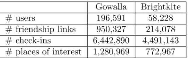
Gowalla Brightkite # users 196,591 58,228 # friendship links 950,327 214,078 # check-ins 6,442,890 4,491,143 # places of interest 1,280,969 772,967
Table 6: Number of each type of element in the datasets
user check-in time latitude longitude location id 196514 2010-07-24T13:45:06Z 53.3648119 -2.2723465833 145064 196514 2010-07-24T13:44:58Z 53.360511233 -2.276369017 1275991 196514 2010-07-24T13:44:46Z 53.3653895945 -2.2754087046 376497
Table 7: Sample of check-ins from the Gowalla dataset
Table 6 shows the number of users, friendship links, check-ins, PoIs in each dataset. Tables 7 and 8 are samples of the datasets.
One may wonder why we did not use these two datasets in our previous experiment in section 3. Even if the Gowalla and Brightkite datasets are bigger, they would not be much more significant in this experiment. Indeed, they do not guarantee to comprise location information of all the friends in a user’s social graph because of their collection method. The two dataset from Stanford’s Cho et al. suffering from the same flaw as our Foursquare and Justacot´e datasets, we choose not to use them. Moreover, the Gowalla and Brightkite dataset do not explicitly contain users’ main location. Supporting them would require a pre-processing phase in order to compute users’ main location, by choosing the PoI where they checked in the most often, for instance.
4.2
Inferring social graph through geographic proximity
Here we describe our method to predict users’ social graph using location infor-mation. The algorithm is implemented in Python 3 for the same reasons as in section 3.2.2.
The algorithm takes as input the IDs of two users and the dataset con-taining their check-ins and social graph. It computes the movement vectors corresponding to this users. Components of a user’s vector are representations of the importance this user gives to each PoI he went to. The algorithm may use two distinct measures of importance of PoIs to build users’ vectors. The first
user check-in time latitude longitude location id 58186 2008-12-03T21:09:14Z 39.633321 -105.317215 ee8b88dea22411 58186 2008-11-30T22:30:12Z 39.633321 -105.317215 ee8b88dea22411 58186 2008-11-28T17:55:04Z -13.158333 -72.531389 e6e86be2a22411
measure is simply the count of how many times the corresponding user checked in at a PoI. Although it is a very basic measure, it has the advantage of being quick to compute. Thus it gives an approximate idea of which PoIs characterise the best a user, in a short amount of time. When we know this information, we can assume that two users having more or less the same characteristic PoIs could be friends.
The second measure is an adaptation of the term frequency-inverse document frequency (tf*idf) weight. In the field of information retrieval, tf*idf is used to measure importance of a term in a corpus of texts.
• The term frequency of a term t in a document d is the number of appearances of t in d, normalised by the total number of words in d. Normalisation avoids favouring long texts over short ones.
tf(t, d) = |∀x ∈ d : x = t| |d|
• The inverse document frequency of a term t in a corpus c is the total number of documents in c divided by the number of documents in c which contain t. We use the logarithm of this quotient to reduce the scope of all possible values. The logarithm’s base is not important here as long as we use the same for all measures. We choose the natural logarithm because Euler’s constant e is Python’s default base for the logarithm. This way, idf measures the rareness of t in all the documents of c.
idf(t, c) = log |c| |∀d ∈ c : t ∈ d|
So the tf*idf weight of a term t in a document d among a corpus of texts c is given by the multiplication of the term frequency and the inverse document frequency, hence the use of an asterisk in term frequency-inverse document frequency notation.
tf∗ idf (t, d, c) = tf (t, d) × idf (t, c) We adapt the tf*idf weight by replacing term by check-in2
, document by place and corpus by the full set of places of a dataset. This gives us :
• cf (c, p), the check-in frequency of a check-in c at a place p. It measures the importance of a place for a user.
• ipf (c, s), the inverse place frequency of a check-in c in a set of places s. It calculates the inverse of the frequency of the check-in class of c in s. In other words, it measures the popularity of a place among all users of our datasets.
2
Please note that every time we mention a check-in in this paragraph, it is done by the same user. We do not take into account the timestamp of the check-ins. We consider all the check-ins done at a place to be the same, independently from their date.
• cf ∗ ipf (c, p, s), the check-in frequency-inverse place frequency of a check-in c at a place p among the full set of places of a dataset s. It measures the importance of p for the user doing c by pondering his frequency of chech-in at p by the popularity of p among all users of the concerned geosocial network.
Our cf*ipf measure is more refined than counting the number of check-ins at a place because it accounts for the popularity of a place. Indeed, if the place where a user checks in the most often is a very popular place where many other users check in too, it is not a very useful place for characterising this user. So cf*ipf gives higher values to less common places where the user checks in often. Then, the algorithm evaluates to what extent the input users are similar using their movement vectors. We use the cosine similarity measure for that purpose. It measures the similarity of two vectors as the cosine of the angle between them. This measure is based on the scalar product. Indeed, the corre-sponding formula being v1· v2 = kv1kkv2k cos θ, we easily derive the cosine of the angle between two vectors formula, i.e. the cosine similarity formula :
cosθ= v1· v2 kv1kkv2k
We choose this similarity measure because it is well-known and often used [SB88]. Moreover, it is convenient because it takes vectors as input and it is simple to implement.
Finally, the algorithm predicts whether the two input users are likely to be friends or not by comparing the cosine similarity of their movement vectors. If the users’ similarity is significantly above the average similarity between users, it predicts that the users are probably friends. We consider that a similarity four times above the average is significant enough to say that the concerned users do not share the same characteristic places by chance. So they must have some kind of social relationship.
Given the large sizes of our datasets, we precompute several elements which require a sizable amount of time to be calculated. One element which we pre-compute is movement vectors of users. The other element which we prepre-compute is similarities between users. We discuss complexity and computation time prob-lems in section 4.4.
4.3
Application to the Gowalla and Brightkite datasets
4.3.1 Results
Our results make use of 51,406 users (88.2 %) from the Brightkite dataset and 107,092 users (54.5 %) from the Gowalla dataset. These numbers differ from the total number of users found the the datasets because not all users made a public check-in during the collection period. Some users are present in the datasets only because they are part of the social graph of a user who made a public check-in.
Gowalla Brightkite Average similarity w/ check-in count vectors 0.00020015176402377792 0.0013966922250071398 Average similarity w/ cf*ipf 8.455772843998304e-05 0.0008765490810133199 Table 9: Average values of similarity between two users in Gowalla and
Brightkite
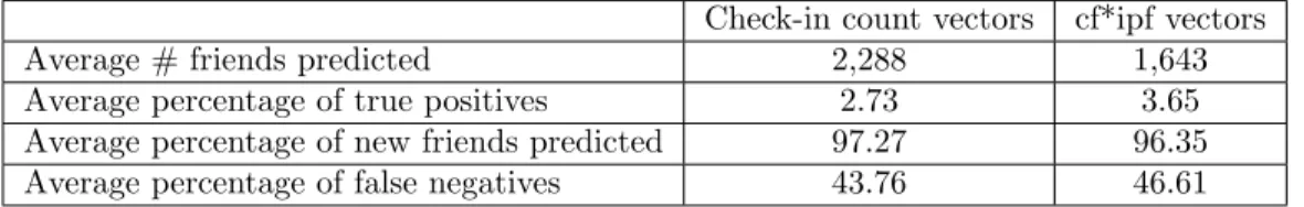
Check-in count vectors cf*ipf vectors Average # friends predicted 2,288 1,643 Average percentage of true positives 2.73 3.65 Average percentage of new friends predicted 97.27 96.35 Average percentage of false negatives 43.76 46.61
Table 10: Efficiency of place importance measures in Brightkite
Table 9 shows that the similarity between any two users is low. It is logical because when randomly picking two users, chances that they are friends are very low. Average similarities using cf*ipf vectors are also smaller because values corresponding to check-ins in popular places are reduced by the cf*ipf weighting.
Given the complexity issues described in section 4.4 that we faced, we only have partial results. Table 10 use a sample of 30 users to compare our results depending on the type of vector used. The similarities between these 30 tar-get users and all the 51,406 users of Brightkite are evaluated to predict their friendship status. The check-in count measure produces more potential friends. Among these predicted friends, a greater share (97.27 %) is users which do not originally appear as friends of the target users.
To assess the reliability of our predictor, we compare the predictions to the ground truth. Doing so shows several things. The check-in count measure has a better recall with 43.76 % of actual friends that the predictor classifies as not friends. 43.76 % of false negatives is not necessarily an issue because not all friendships come from mutual PoIs. Indeed, one can make new friends among users he does not usually see in his favourite PoIs. In [SNM11], they find that 30 % only of new friendship links are created between users sharing PoIs. So our predictor seems to perform better than theirs as it correctly classifies 52.24 % of the target users’ actual friends. Regarding the prediction’s precision, the cf*ipf measure is better suited with 3.65 % of all the predicted friends being actual friends. This confirms the intuition that predictions based on a more accurate measure of importance of PoIs contain greater part of correct results.
4.4
Complexity and computation time
When running this experiment, we had to deal with problems of complexity of our calculations. Indeed, the volume of data we manipulate is such that the time and memory space needed easily become unreasonable. As a proof, despite
u1 u2 . . . un−1 un u1 simil(u1, u1) simil(u1, u2) . . . simil(u1, un−1) simil(u1, un) u2 simil(u2, u1) simil(u2, u2) . . . simil(u2, un−1) simil(u2, un)
..
. ... ... . .. ... ... un−1 simil(un−1, u1) simil(un−1, u2) . . . simil(un−1, un−1) simil(un−1, un)
un simil(un, u1) simil(un, u2) . . . simil(un, un−1) simil(un, un) Table 11: Model of a similarity matrix
having access to a powerful server3
to run our calculations, all predictions of friendship regarding any pair of user are not done computing at the time of writing.
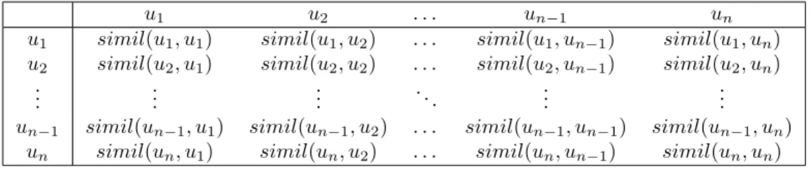
The main issue relates to similarity matrices. We need to know the average value of similarity between users for our friendship predictor. Even though we must do this calculation only once, it requires to be able to access similarity values in a structured manner to avoid accounting several times for the same value. We do this via similarity matrix. This is a symmetric matrix which allows to get the similarity of any pair of users. Table 11 illustrate what similarity matrices look like.
The problem comes from the size of these matrices. Indeed, the similarity matrices based on check-in count vectors and cf*ipf vectors contain 58, 2282
= 3, 390, 499, 984 values for Brightkite and 196, 5912
= 38, 648, 021, 281 values for Gowalla. Moreover, the similarity values are implemented with the float type which requires more memory space than the integer type for instance. Ob-viously, these matrices cannot fit in RAM as is. We are then forced to use serialisation to unload the RAM to the hard drive while the programme is com-puting.
Even though we manage RAM usage, our problems are not solved. Despite a space-efficient method of storage as claimed in the documentation of Python’s serialisation module, all the vectors and similarities from Brightkite and Gowalla require 900+ Gio. While serialisation is beneficial for RAM use, it also impacts negatively computation time by adding disk access time.
We mention potential solutions to manage scalability and complexity in sec-tion 5.2
5
Conclusion
5.1
Discussion on the results
The goal of this work is to expose the implications in terms of privacy of pro-viding location information in a social network context. Social networks imply risks for their users’ privacy. Disclosing one’s current location or traces of one’s previous movements brings another kind of privacy risk as location is a very
3
sensitive and private information. But does using location in social networks imply privacy risks that are only the sum of the two preceding types of risks? Or does it create in addition a new type of risks, appearing when location and social networking are combined?
We sketched the beginning of an answer to this question and it seems that geosocial networks create a new type of risks. Indeed, section 3 shows an al-gorithm classifying users depending on whether their friends live close or far away from them. It allows to create geolocated targeted advertisement and it comes in complement of algorithms inferring a user’s main location based on their friends location. While these two applications are not significant breaches of privacy, and even though this experiment is not a proof because of the not significant enough datasets used, it at least has the benefit of showing the exis-tence of attacks made possible thanks to the combination of location and social networking.
Our experiment of section 4 also points towards the same conclusion. Using check-ins, the corresponding algorithm is able to recover a partial social graph from zero, while other algorithms could not do so. An exception would be the algorithm in [LCB10] which, similarly to us, use an additional information to build a social graph. Inferring a users’ social graph is indeed an attack on privacy because beyond the simple knowledge of who his friends are, an adversary in possession of a social graph can conduct further inference attacks on that graph to deduce properties about its nodes, as shown in [ZG09]. Thus, even if a users’ social graph is invisible to third parties, he must be careful about its check-ins or it might render useless his social graph’s protection.
5.2
Possible future work
This work may be extended in several ways. Obviously, it would benefit from being completed with datasets collected with this purpose in mind. Such dataset would contain as many check-ins as possible and most importantly, the full social graphs of the target users.
In the same goal of consolidation, tools for managing scaling up of datasets should be used. Such tools could be the SNAP network analysis library, which claim to be effective even with massive networks. Another tool which deserve some investigation is Apache Hadoop, a framework implementing the MapRe-duce algorithm for big data processing.
The next step in developing section 3’s algoritm is to predict the target user’s main location based on his friends’ ones. Modification of the algorithm towards this goal should not be too complex. It only requires to alter the last step of our algorithm. Indeed, the predictor would co-locate the target user with one of his friends as in [BSM10]. It would choose which friend by taking the median one. Here, by median friend we mean the friend which minimises the distance between itself and all the other ones. Moreover, it would be possible to compare the predicted location to the ground truth thanks to our datasets.
Another work worth pursuing is to use temporal information and correlation of check-ins. This aspect of check-ins is neglected in this current work but it
could add useful information. For instance, two users may have similar move-ment vectors but they may actually not know each other because they check in at totally different times. Similarly, the geographic distance between PoIs should be taken into account. Indeed, if a user checks in at two distant PoIs within a small time frame, it means something unusual is going on. It could be the sign of an adversary conducting an attack.
Finally, one could develop a fallback method using badges (or any other form a virtual achievement) to deduce a user’s movements when his check-ins are not available. Indeed, some badges are linked to particular events like a music festival or specific places such as the Eiffel tower. These information, despite being coarsers than check-ins, may already reveal sensitive information about the concerned user.
References
[AGS11] Chid Apt´e, Joydeep Ghosh, and Padhraic Smyth, editors. Pro-ceedings of the 17th ACM SIGKDD International Conference on Knowledge Discovery and Data Mining, San Diego, CA, USA, Au-gust 21-24, 2011. ACM, 2011.
[BE07] Danah M. Boyd and Nicole Ellison. Social network sites: Definition, history, and scholarship. J. Computer-Mediated Communication, 13(1):210–230, 2007.
[Bec] Brian Beck. geopy. code.google.com/p/geopy.
[BSM10] Lars Backstrom, Eric Sun, and Cameron Marlow. Find me if you can : Improving geographical prediction with social and spatial proximity. North, (WWW ’10):61, 2010.
[CML11] Eunjoon Cho, Seth A. Myers, and Jure Leskovec. Friendship and mobility: user movement in location-based social networks. In Apt´e et al. [AGS11], pages 1082–1090.
[Com] Creative Commons. Creative commons attribution 3.0 licence. creativecommons.org/licenses/by/3.0.
[GG03] Marco Gruteser and Dirk Grunwald. Anonymous usage of location-based services through spatial and temporal cloaking. In Proceed-ings of the 1st international conference on Mobile systems, appli-cations and services, MobiSys ’03, pages 31–42, New York, NY, USA, 2003. ACM.
[GKdPC10] S´ebastien Gambs, Marc-Olivier Killijian, and Miguel N´u˜nez del Prado Cortez. Show me how you move and i will tell you who you are. In Elisa Bertino, Maria Luisa Damiani, and Y¨ucel Saygin, editors, SPRINGL, pages 34–41. ACM, 2010.
[Gmb] Qype GmbH. Qype. www.qype.com.
[Gro] CCM Benchmark Group. Copains d’avant. copainsdavant. linternaute.com.
[LCB10] Vincent Leroy, B Barla Cambazoglu, and Francesco Bonchi. Cold Start Link Prediction, pages 393–402. ACM, 2010.
[Les] Jure Leskovec. Stanford large network dataset collection. snap. stanford.edu/data/index.html#locnet.
[LnK07] David Liben-nowell and Jon Kleinberg. The link-prediction prob-lem for social networks. J. American Society for Information Sci-ence and Technology, 58(7):1019–1031, 2007.
[PDH08] Andreas Pfitzmann, Tu Dresden, and Marit Hansen. Anonymity, unlinkability, undetectability, unobservability, pseudonymity, and identity management – a consolidated proposal for terminology, 2008.
[Pot11] Christophe Potin. Analyse de protection de la vie priv´ee et de s´ecurit´e de r´eseaux sociaux g´eo-localis´es, 2011.
[Ric] Leonard Richardson. Beautiful Soup. www.crummy.com/software/ BeautifulSoup.
[SB88] Gerard Salton and Christopher Buckley. Term-weighting ap-proaches in automatic text retrieval. In INFORMATION PRO-CESSING AND MANAGEMENT, pages 513–523, 1988.
[SG12] et al. S´ebastien Gambs. De-anonymization attack on geolocated datasets, 2012. Submitted.
[SNM11] Salvatore Scellato, Anastasios Noulas, and Cecilia Mascolo. Ex-ploiting place features in link prediction on location-based social networks. In Apt´e et al. [AGS11], pages 1046–1054.
[Swa] Jon Swartz. The latest from gowalla is worth checking out. content.usatoday.com/communities/technologylive/post/2010/12/the-latest-from-gowalla-is-worth-checking-out/1.
[Tso] Alexia Tsotsis. Foursquare now officially at 10 million users. techcrunch.com/2011/06/20/ foursquare-now-officially-at-10-million-users.
[UKBM11] Johan Ugander, Brian Karrer, Lars Backstrom, and Cameron Marlow. The anatomy of the facebook social graph. CoRR, abs/1111.4503, 2011.
[VFBJ11] Carmen Ruiz Vicente, Dario Freni, Claudio Bettini, and Chris-tian S. Jensen. Location-related privacy in geo-social networks. IEEE Internet Computing, 15(3):20–27, 2011.
[Vin75] Thaddeus Vincenty. Direct and inverse solutions of geodesics on the ellipsoid with application of nested equations. Survey Review, 23(176):88–93, 1975.
[ZG09] Elena Zheleva and Lise Getoor. To join or not to join: the illusion of privacy in social networks with mixed public and private user profiles. In Juan Quemada, Gonzalo Le´on, Yo¨elle S. Maarek, and Wolfgang Nejdl, editors, WWW, pages 531–540. ACM, 2009.