Analyse génomique de la sélection spatialement variable chez
l’anguille d’Amérique (Anguilla rostrata)
Mémoire
Charles Babin
Maîtrise en biologie
Maître ès sciences (M. Sc.)
Québec, Canada
© Charles Babin, 2017
Analyse génomique de la sélection spatialement variable chez
l’anguille d’Amérique (Anguilla rostrata)
Mémoire
Sous la direction de :
iii
Résumé
L'anguille d'Amérique est un poisson avec un cycle de vie très particulier. En effet, elle occupe une aire de répartition qui s'étire du Groenland aux Caraïbes, mais tous les individus se reproduisent dans la mer des Sargasses. Après la reproduction, les larves sont dispersées de façon aléatoire jusqu'aux côtes. Ce lieu de reproduction unique fait en sorte que tous les individus de l'espèce appartiennent à la même population. Par contre, les conditions environnementales varient grandement au sein de l'aire de répartition, puisque celle-ci s'étend de régions subarctiques à des régions subtropicales, ce qui confronte les individus à des conditions différentes selon l'endroit jusqu'où ils dérivent et peut entraîner la sélection d'allèles différents selon les régions. Les objectifs de cette étude étaient d'identifier les régions du génome soumises au phénomène de sélection spatialement variable et quels mécanismes sont affectés par la sélection. Pour ce faire, 710 individus en provenance de 13 sites différents représentant une grande partie de l'aire de répartition de l'espèce ont été séquencés. Un total de 12 098 SNP a été obtenu. Des méthodes d'association environnementale et d'analyse de redondance ont été employées pour identifier des marqueurs potentiellement sous sélection spatialement variable. Un total de 183 marqueurs a été identifié comme étant sous sélection spatialement variable. L'interaction entre les différentes régions sous sélection a également été évaluée en utilisant des scores polygéniques additifs. Des corrélations significatives entre ces scores polygéniques et la latitude, la longitude et la température ont été identifiées. Finalement, nous avons identifié les gènes à proximité des marqueurs potentiellement sous sélection. Parmi ces gènes, le mécanisme de réponse à l'insuline était le seul mécanisme significativement enrichi. Cette étude a permis de mieux documenter l'étendue de la sélection spatialement variable chez l'anguille d'Amérique en montrant qu’il semble y avoir de la sélection dans de nombreuses régions du génome.
iv
Abstract
The American eel is a fish with a complex life cycle. The eel occupy a wide species range from Greenland to the Caribbean, but all eels reproduce in the Sargasso Sea. After the reproduction, the larvea are advected randomly to the coast by ocean currents. Because of this reproduction mode, all the American Eel are in the same population. On the other hand, the range is extending from subarctic to subtropical regions and the eels occupying these different regions are facing really different environmental conditions. These differents conditions could result in the selection of different alleles. The objective of this study was to identify the different regions of the genome that are affected by this phenomenon of spatially-varying selection and which mecanisms are affected by selection. A total of 710 glass eels captured in 12 different sites representing an important part of the species range were sequenced to reach these objectives. After sequencing, 12 098 SNPs were conserved for further analysis. Using environmental association and redundancy analyses approaches, 183 of these markers were identified to be potentially under spatially-varying selection. The interaction between these differents regions was analyzed using additive polygenic scores. Significant correlations were identified between these polygenic scores and the latitude, longitude and temperature. Genes close to outliers were identified and gene ontology analyses were made. The only significantly enriched pathway was the insuline signalling pathway. With this study our understanding of the spatially-varying selection in the American Eel has been increased.
v
Table des matières
Résumé ... iii
Abstract ... iv
Table des matières ... v
Liste des tableaux ... vi
Liste des figures ... vii
Remerciements ... viii
Avant-propos ... x
Introduction ... 1
Forces évolutives... 1
Panmixie... 2
Techniques de séquençage de nouvelle génération ... 3
Anguille d'Amérique ... 3
Cycle vital ... 3
Sélection spatialement variable ... 5
Déclin des populations d'anguilles ... 7
Objectif du projet ... 7
Chapter 1: RAD-seq reveals patterns of additive polygenic variation caused by spatially-varying selection in the American Eel (Anguilla rostrata) ... 9
Résumé ... 10
Abstract ... 11
Conclusion ... 38
Identification de marqueurs potentiellement sous sélection spatialement variable ... 38
Effet additif des marqueurs potentiellement sous sélection ... 39
Fonctions enrichies chez les marqueurs potentiellement sous sélection ... 40
vi
Liste des tableaux
Table 1 Names and codes of sampling locations, number of individuals per site, latitude, longitude,
river mouth temperature and sampling year. Temperatures for 2008 are the average sea-surface temperature near the river mouth during the 10 days prior to the sampling day during recruitment. Temperatures for 2009 are the average sea-surface temperature of the river mouth during the sampling month………18
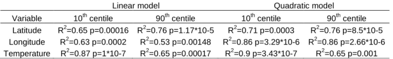
Table 2 Correlation coefficients and p-values of the relationship between the 10th and 90th centile of the polygenic scores of each of the sampling sites and the environmental variables. The correlation coefficient and p-values were calculated following a quadratic and a linear model………27
vii
Liste des figures
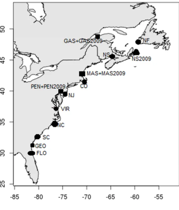
Figure 1 Location map of the 13 sampling sites where American glass eels were collected for this
study. Labels correspond to the site codes provided in table 1. The sites identified by squares were sampled in 2008 and 2009, sites identified by circles were sampled in 2008 and the site identified by a triangle was sampled in 2009………..16
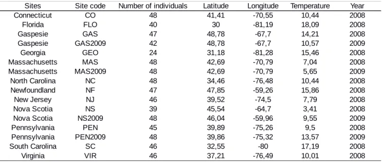
Figure 2 (A) Redundancy analysis (RDA) performed with 12 098 filtered SNPs, using latitude,
longitude, temperature and year as constraining variables. (B) Redundancy analysis performed using the 197 SNPs detected to be potentially affected by selection with the RDA outlier detection approach (C) Redundancy analysis performed using the 90 markers significantly associated with environmental variables in Bayenv2 analysis. Only the first 2 axes are shown for each RDA. Sites are identified by their code (Table 1) and by colored points reflecting water temperature value, from yellow for colder sites to dark red for warmer sites. The direction of main variation for each of the 4 constraining variables (Year, Latitude, Longitude, Temperature) is indicated by a blue vectors. SNPs contributions appear as red '+' symbols. The proportion of total variance explained by each axis is indicated in percent………24
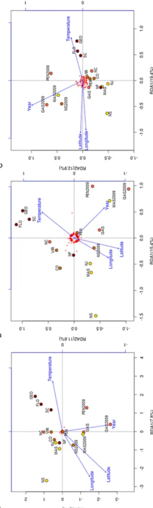
Figure 3 Histograms of the number of outliers detected in 100 simulations for the different
environmental variables; latitude (A), longitude (B), temperature (C) and year (D). The x axis represents the number of outliers detected in a run. The y axis represents the number of simulations that detected this number of outlier. The vertical black bar represents the average number of outlier detected in the runs made with the real dataset. Note that the number of outliers detected in each run was higher than the number of outliers used for further analyses as reported in the main text. This is because not always the same outliers were detected in each run and in order to remain conservative in downstream analyses, we retained only the markers that were significant in 6 runs or more out of 12……….26
Figure 4 Correlations between additive individual polygenic scores based on all 259 outlier markers
and each of 3 explanatory variables: latitude (A), longitude (B) and temperature (C). Additive polygenic scores were obtained at the individual level by summing the number of locally favourable alleles. Correlation coefficients and p-values of the quadratic correlation model are shown at the top of each panel………28
viii
Remerciements
J'ai toujours été curieux et je me suis toujours intéressé aux sciences. Au secondaire, les cours de biologie étaient parmi mes favoris surtout lorsqu'on parlait de l'évolution et de la génétique mendélienne. Je trouvais fascinant que l'alternance de 4 molécules chimiques puisse résulter en des organismes aussi différents que les virus, les bactéries, les méduses ou les champignons. Je trouve encore mystérieux que toute cette diversité ait pu évoluer simplement par le jeu des mutations. Lorsque le temps est venu de m'inscrire à l'université, je me suis dit que je pourrais poursuivre mes études en biologie pour assouvir ma soif de connaissances et ma curiosité par rapport aux questions de génétique.
Au cours de mon baccalauréat, j'ai voulu voir à quoi ressemblait la recherche et j'ai donc contacté Louis pour voir si je pouvais faire un stage dans son laboratoire afin de le découvrir. Louis me connaissait déjà, car j'ai côtoyé deux de ses fils au sein des scouts pendant une dizaine d'années. Il m'a offert de travailler au laboratoire durant l'été, si j'obtenais une bourse du CRSNG. J'ai obtenu la bourse et j'ai pu découvrir les rudiments du travail de laboratoire en aidant Simon Bernatchez dans son projet de maîtrise portant sur le touladi. J'ai beaucoup aimé faire du laboratoire et j'ai voulu faire une initiation à la recherche dans le cadre de mon bac. Le projet qui m'avait été confié était toutefois de grande ampleur et a fini par devenir la maîtrise dont vous allez lire le mémoire dans les prochaines pages.
J'aimerais remercier mon directeur Louis Bernatchez de m'avoir permis de faire partie de son laboratoire formés d'étudiants de très haut niveau qui m'ont permis de progresser grandement. Je le remercie également d'avoir cru en moi en me confiant un projet de séquençage de nouvelle génération avec des centaines d'individus alors que je n'étais qu'un étudiant au bac.
J'aimerais remercier Scott Pavey, qui m'a montré comment me servir d'un terminal et comment me débrouiller dans les méandres de la bio-informatique. Il m'a également aidé à développer la méthode que nous avons utilisée pour identifier nos marqueurs. Le génome de l'anguille d'Amérique qu'il a assemblé a grandement facilité les analyses.
Mon collaborateur Pierre-Alexandre Gagnaire a contribué de façon importante aux analyses en me faisant des suggestions d'analyses à réaliser et en m'aidant à interpréter les résultats qui ont découlé de
ix
ces analyses. Il m'a également aidé à mieux comprendre les analyses.
Pour la partie laboratoire, j'aimerais remercier Clément Rougeux qui m'a aidé lors de la préparation des librairies en vue du séquençage. J'aimerais également remercier tous les autres membres du laboratoire qui m'ont permis de mener mon projet de maîtrise à bon port en faisant des suggestions.
Finalement, j'aimerais remercier ma famille qui m'a toujours encouragé à poursuivre mes études et m'a permis de développer ma curiosité.
x
Avant-propos
L'article qui figure à l'intérieur de ce mémoire s'intitule « RAD-seq reveals patterns of additive polygenic variation caused by spatially-varying selection in the American Eel (Anguilla rostrata)». Il a été publié par le journal Genome Biology and Evolution dans son volume 9 issue 11 (https://doi.org/10.1093/gbe/evx226).
Les coauteurs de cet article sont Pierre-Alexandre Gagnaire, Scott Pavey et mon directeur Louis Bernatchez. Je suis l'auteur principal de l'article.
Pierre-Alexandre Gagnaire a contribué à l'analyse et à l'interprétation des résultats. J'ai effectué le travail de laboratoire ainsi que l'analyse et l'interprétation des résultats. J'ai aussi écrit le manuscrit. Tous les auteurs ont contribué à l'amélioration et à la révision du manuscrit.
1
Introduction
Forces évolutives
L'évolution est contrôlée par 4 forces évolutives. Trois d'entre elles sont neutres, la mutation, la dérive génétique et la migration. Elles sont dites neutres, car elles n’agissent pas de manière adaptative. Les mutations apparaissent de façon aléatoire un peu partout dans le génome et sont le moteur de l'évolution. Pour sa part, la dérive génétique fait varier stochastiquement à chaque génération la fréquence allélique des marqueurs au sein d'une population de façon plus ou moins importante en fonction de la taille effective de celle-ci. Elle engendre généralement une différenciation entre les populations, car les variations de fréquence allélique diffèrent entre les populations, puisqu'elles sont aléatoires et dépendent de la taille effective qui varie entre les populations. Les populations avec une taille effective moins importante vont avoir des fréquences alléliques qui vont varier de façon plus importante que celles avec une plus grande taille effective. La migration permet quant à elle d'échanger des allèles entre les populations, ce qui réduit la différenciation entre celles-ci. Plus le flux génique est important entre 2 populations, moins elles seront différenciées l'une de l'autre. La migration a donc un effet inverse de celui de la dérive génétique en homogénéisant les populations entre elles. La quatrième force évolutive, la sélection naturelle, est quant à elle dite directionnelle, car elle agit seulement sur quelques régions du génome en faisant varier en fréquence les marqueurs avantageux ou désavantageux dans certaines conditions, tout en n'affectant pas les autres. Les marqueurs sous sélection varient en fonction des pressions exercées par l'environnement et ne sont souvent pas les mêmes dans les différentes populations d'une même espèce, puisqu'elles ne sont pas confrontées aux mêmes conditions environnementales. Les phénotypes qui sont avantageux dans certaines conditions peuvent ainsi être sélectionnés (Herron et Freeman, 2014).
La sélection naturelle peut s'exercer de différentes façons. Si elle favorise les phénotypes dans une direction précise, elle sera dite directionnelle. Si les phénotypes qui sont favorisés sont les plus extrêmes, elle sera dite divergente, car les phénotypes moyens seront sélectionné de façon négative. Lorsque ce sont plutôt les phénotypes moyens qui sont favorisés, la sélection est stabilisatrice. La pression de sélection dépend également de l'avantage sélectif de l’allèle. Si la mutation est très avantageuse pour les individus qui la portent, sa fréquence allélique augmentera plus rapidement que
2
celle d'une mutation qui procure moins d'avantages à son porteur. Les mutations qui sont fortement désavantageuses pour leurs porteurs seront de leur côté très négativement sélectionnées, car leurs porteurs auront de la difficulté à se reproduire, ce qui diminuera leur fréquence allélique de façon importante (Mitchell-Olds et al., 2007).
Panmixie
La plupart des espèces sont composées de plusieurs populations avec plus ou moins de connectivité entre elles. Les populations sont plus ou moins différenciées les unes des autres selon leur degré de connectivité. Elles s'adaptent souvent aux conditions présentes dans leur environnement, ce qui peut résulter en l'apparition d'adaptations locales au sein de celles-ci, après plusieurs générations de sélection pour les mêmes allèles. Ces adaptations locales procurent aux individus locaux un meilleur fitness dans les conditions locales comparativement à celui d'individus en provenance d'autres habitats soumis à ces mêmes conditions (Kawecki et Ebert, 2004). Toutefois, certaines espèces ne sont formées que d'une seule population. Chez ces espèces, le flux génique est si important qu'il prévient la différenciation entre les individus et empêche l'apparition d'une structure de populations. Ces espèces sont dites panmictiques, car la reproduction se fait à l'échelle de l'espèce de façon aléatoire (Wapples et Gaggiotti, 2006). Le développement d'adaptations locales chez les espèces panmictiques est impossible à cause de l'absence de structure de populations qui fait en sorte que les allèles se propagent librement au sein de l'aire de répartition de l'espèce. Malgré la sélection qui s'opère sur certains marqueurs avantageux dans une région de l'aire de répartition, il n'y a aucune barrière qui empêche les allèles qui sont avantageux ailleurs de parvenir jusqu'à cette région et les allèles avantageux dans ce site de parvenir à d'autres sites où ils seront moins avantageux (Kawecki et Ebert, 2004). Les travaux de Levene (1953) ont toutefois démontré que la sélection balancée peut maintenir un polymorphisme chez certains marqueurs, lorsque différents allèles sont favorisés au sein de différentes niches écologiques. Le polymorphisme peut ainsi se maintenir au sein d'espèces panmictiques à cause de la mortalité différentielle des individus en fonction de leur génotype dans les différents habitats. Cette mortalité différentielle fait en sorte que les fréquences alléliques peuvent varier en fonction des conditions environnementales, malgré l'absence de structure, car certains allèles seront plus avantageux dans certaines conditions et leurs porteurs auront donc un meilleur taux de survie. On nomme ce phénomène sélection spatialement variable en panmixie. Les anguilles sont de bons exemples de ce phénomène (Gagnaire et al., 2012).
3
Techniques de séquençage de nouvelle génération
Depuis quelques années, la biologie moléculaire a été profondément transformée par l'arrivée des techniques de séquençage de nouvelle génération, qui ont permis une augmentation exponentielle des données à un coût relativement faible. En effet, jusqu'à récemment les études sur les organismes non modèles ne portait que sur quelques dizaines de marqueurs microsatellites à la fois, car il fallait développer des amorces pour chacun des marqueurs, ce qui prenait énormément de temps et coûtait assez cher. Maintenant, les techniques comme le RAD-sequencing ou le GBS permettent de séquencer des milliers de marqueurs SNP répartis un peu partout dans le génome sans avoir à faire de développement au préalable. Elles consistent à uniquement séquencer les régions voisines de site de restriction. Ces techniques permettent de séquencer seulement une partie du génome, ce qui réduit grandement les coûts de séquençage (Metzker, 2010). Cette augmentation du nombre de marqueurs analysés permet de scruter une plus grande partie du génome et donc de faire des analyses de génétique des populations plus précises. Il est également plus facile d'identifier des marqueurs potentiellement sous sélection et les mécanismes physiologiques qui sont affectés par ces phénomènes avec les nouvelles techniques de séquençage, puisque beaucoup plus de régions du génome sont examinées qu'auparavant. Les régions du génome soumises à la sélection ont donc plus de chances d'être séquencées et l'utilisation de plus de marqueurs permet de mieux évaluer la structure des populations. La réduction des coûts de séquençage a également permis l'assemblage d'un grand nombre de génomes au cours des dernières années. La disponibilité d'un génome de l'espèce étudiée ou d'une espèce proche permet de faciliter les différentes analyses bioinformatiques et de mieux identifier les gènes impliqués dans les processus d'adaptation en permettant de localiser précisément les marqueurs par rapport aux gènes (Ellegren, 2014).
Anguille d'Amérique
Cycle vital
L'anguille d'Amérique (Anguilla rostrata) est une espèce de poisson catadrome présente en Amérique, du Groenland aux Antilles et tout le long de la côte atlantique. Le cycle de vie de l'anguille est très complexe. Tout d'abord, toutes les anguilles d'Amérique naissent dans la mer des Sargasses dans l'océan Atlantique. Peu après leur éclosion, les larves se métamorphosent en leptocéphales. Ces larves
4
sont plates comme des feuilles. Cette forme leur permet de se laisser dériver au gré des courants marins jusqu'à la côte américaine (Vélez-Espino et Koops, 2010). Une fois sur le plateau continental, les leptocéphales se transforment en civelles, qui sont des larves cylindriques et transparentes. Arrivées sur la côte, elles peuvent y rester pour vivre en eau salée, aller vivre en eau saumâtre dans les estuaires ou remonter les cours d'eau pour passer leur vie en eau douce. Au cours de leur croissance, les anguilles deviendront d'abord des anguillettes, puis finiront par se pigmenter pour devenir des anguilles jaunes. C'est sous cette forme qu'elles passeront la majorité de leur vie. Après quelques années, elles se métamorphoseront de nouveau pour devenir cette fois des anguilles argentées. C'est à ce stade que les anguilles deviennent matures sexuellement. Sous cette forme, elles feront le chemin inverse vers la mer des Sargasses pour s'y reproduire et y mourir (Jessop, 2010).
Le cycle de vie des anguilles est longtemps resté mystérieux. En effet, la reproduction de l'anguille d'Amérique n'a jamais été observée et aucune adulte n'a jamais été vu dans la mer des Sargasses. La migration des adultes vers la mer des Sargasses pour s'y reproduire n'a pu être confirmée que très récemment en suivant la trajectoire vers la mer des Sargasses d'une anguille argentée femelle qui avait été marquée (Béguer-Pon et al., 2015). La mer des Sargasses avait auparavant été identifiée comme lieu de reproduction potentiel de l'espèce, car c'est à cet endroit que les leptocéphales les plus petites avait été capturées (Hanel et al., 2014). L'anguille d'Amérique partage son aire de reproduction avec son espèce sœur, l'anguille européenne (Anguilla anguilla). L'anguille européenne a un mode de vie et un cycle de vie similaire à l'anguille d'Amérique, mais elle passe la partie continentale de son cycle de vie en Europe et en Afrique du nord. Des hybrides entre les 2 espèces ont d'ailleurs été identifiés en Islande (Albert et al., 2006).
La durée de vie des anguilles d'Amérique varie beaucoup selon la latitude à laquelle les individus vont vivre et selon leur sexe (Jessop, 2010). En effet, les mâles atteignent le stade d'anguille argentée à une plus petite taille que les femelles. Ils sont aussi moins âgés lorsqu'ils atteignent ce stade. Le taux de croissance annuel des anguilles diminue avec l'augmentation de la latitude, car la saison de croissance diminue également avec celle-ci à cause de la diminution de la température. L'âge à la maturité augmente avec la latitude, passant de 5 ans pour les régions les plus au sud à plus de 20 ans pour les régions les plus au nord chez les femelles. Chez les mâles, il passe de 5 ans au sud à 13 ans au nord. Les mâles atteignent la même longueur peu importe la latitude, tandis que la longueur des femelles augmente avec la latitude. Les femelles sont en moyenne 2 fois plus longues que les mâles lorsqu'elles
5
sont matures. Les individus les plus grands de l'espèce sont les femelles du fleuve Saint-Laurent et des Grands Lacs, qui grandissent lentement et durant très longtemps. Le taux de croissance varie également selon l'habitat des anguilles. En effet, les anguilles d'eau salée ou d'eau saumâtre ont un taux de croissance plus grand que des anguilles vivant dans les habitats d'eau douce à proximité et qui sont donc soumis à des températures semblables (Cairns et al., 2009). La répartition des sexes est également fort différente selon les sites. Certains sites ne comprennent que des mâles ou des femelles, alors que d'autres sites comprennent autant de mâles que femelles (Oliveira et al., 2001). De leur côté, les facteurs déterminant le sexe chez l'anguille ne sont pas clairement identifiés. Différents facteurs environnementaux ont été proposés, comme la densité de population, la température de l'eau, le taux de croissance initial des individus, l'habitat, le taux de salinité ou la latitude. Les études se contredisent toutefois entre elles à ce propos (Davey et Jellyman, 2005).
Sélection spatialement variable
Puisque que toutes les anguilles se reproduisent dans la mer des Sargasses des individus ayant passé leur vie adulte à des milliers de kilomètres se reproduisent ensemble. Ce mode de reproduction empêche la différenciation entre les individus ayant vécu dans différentes régions de l'aire de répartition et fait en sorte que tous les individus de l'espèce appartiennent à une seule et même population. L'anguille d'Amérique est donc une espèce panmictique, même si elle occupe une grande aire de répartition (Côté et al., 2013).
Malgré tout, au cours de leur vie, les individus vont être confrontés à des conditions environnementales assez différentes selon l'endroit où les courants marins vont les transporter. En effet, les Antilles et les régions subarctiques offrent des conditions climatiques assez différentes que ce soit au niveau de la température, de l'ensoleillement ou de la présence de glace. La distance à franchir pour atteindre la côte à partir de la mer de Sargasses varie également beaucoup. Elle varie de 1500 kilomètres pour atteindre la côte de la Géorgie à 5000 kilomètres pour atteindre des régions plus au nord comme la Gaspésie (Jessop, 2010). Ces distances différentes font en sorte que les individus atteignent la côte à un âge différent selon la latitude. En Floride, les civelles arrivent sur la côte en janvier, alors qu'à Terre-Neuve, elles n'arrivent qu'en juillet (Gagnaire et al., 2012). Il y a également des anguilles qui vivent en eau douce, en eau saumâtre et en eau salée. Ces différents milieux confrontent les individus à des conditions distinctes dans lesquelles certains allèles permettront à leurs porteurs de mieux performer,
6
car le phénotype qui en résulte leur procure un avantage dans ce milieu. Cette sélection différentielle fait en sorte que les fréquences alléliques de certains marqueurs favorables dans une région seront plus grandes. Cette sélection sera annulée à chaque nouvelle génération, car le mode de dispersion passif des larves fait en sorte que les individus ont de bonnes chances d'être confrontés à des conditions différentes de celles subies par leurs parents. La sélection opère donc indépendamment à chacune des générations, car un grand nombre d'individus ne seront pas adaptés aux conditions du site où ils se retrouveront et ne survivront donc pas assez longtemps pour aller se reproduire. Les anguilles d'Amérique sont donc probablement l'objet de sélection spatialement variable en panmixie (Pujolar et al., 2014).
La sélection spatialement variable est étudiée chez l'anguille d'Amérique depuis de nombreuses années. En effet, des études ont été réalisées dans les années 70 avec des marqueurs allozymes. Trois marqueurs allozymes avec une fréquence allélique qui était corrélée avec la latitude à laquelle les individus avaient été capturés ont été identifiés comme étant potentiellement sous sélection spatialement variable avec la latitude (Williams et al., 1973). Une autre étude a été effectuée sur une centaine de marqueurs situés dans des régions codantes du génome. Ces marqueurs avaient été préalablement identifiés comme étant les plus différenciés entre des individus en provenance de Floride et de Gaspésie. La fréquence allélique de 13 de ces marqueurs était corrélée avec la température moyenne de l'eau des sites où les anguilles avaient été capturées. Ces marqueurs sont donc potentiellement sous sélection avec la température de l'eau (Gagnaire et al., 2012). Une étude semblable a également été effectuée chez l'anguille européenne. Cette fois-ci, des technologies de séquençage de nouvelle génération ont été employées, ce qui a permis d'utiliser un nombre beaucoup plus important de marqueurs que dans l'étude précédente. Plus de 50 000 marqueurs ont été analysés pour trouver des traces de sélection spatialement variable. Parmi eux, 754 marqueurs ont été identifiés comme étant sous sélection spatialement variable. La fréquence allélique des marqueurs était corrélée avec la température de l'eau des sites d'échantillonnage, la latitude des sites ou leur longitude (Pujolar et al., 2014). Une étude portant l'effet sélectif de la salinité chez l'anguille d'Amérique a permis d'identifier 331 marqueurs parmi les 15 500 analysés, dont la fréquence allélique était lié à la salinité du site où les anguilles avaient été capturées. Plus de 55% de ces marqueurs était presque fixés dans un des 2 milieux malgré la panmixie (Pavey et al., 2015).
7
Déclin des populations d'anguilles
Au cours des dernières décennies, un déclin important des populations a été observé chez plusieurs espèces d'anguilles, comme l'anguille européenne (Anguilla anguilla), l'anguille japonaise (Anguilla
japonica) et l'anguille d'Amérique (Hanel et al., 2014). Chez l'anguille d'Amérique, la diminution la
mieux documentée a été observée dans le fleuve St-Laurent et dans les Grands Lacs. Un déclin de plus de 98% du nombre de juvéniles en montaison a été observéee entre les années 1980 et 2009 au niveau du barrage Moses-Saunders sur le fleuve Saint-Laurent. Ce déclin très important des effectifs a mené à la classification de l'anguille d'Amérique comme espèce menacée au Canada. La pêche commerciale et sportive a été interdite en Ontario et a diminué de façon importante au Québec (COSEPAQ, 2012). De nombreuses causes ont été proposées pour expliquer ce déclin, comme la destruction des habitats potentiels, la surpêche, la présence de barrages nuisant à la migration ou la pollution de l'eau (Castonguay et al., 1994). Des variations climatiques au niveau océanique, comme l'oscillation nord-atlantique ont également été proposées pour expliquer le déclin du nombre d'individus (Côté et al., 2013). Les causes du déclin ne sont toutefois pas encore très bien comprises.
Objectif du projet
L'objectif de ce projet est d'utiliser les techniques de séquençage de nouvelle génération pour étudier la sélection spatialement variable chez l'anguille d'Amérique, afin d'étendre l'étude de Gagnaire et al. (2012) à une plus grande partie du génome pour mieux documenter le phénomène de sélection spatialement variable chez cette espèce. Étudier une plus grande du génome permet de voir à quelle échelle la sélection spatialement variable s’effectue. Pour ce faire, les mêmes variables environnementales, la latitude, la longitude et la température de l'eau ont été employées pour détecter si des marqueurs étaient sous sélection avec celles-ci. De plus, l'utilisation d'individus capturés au même endroit lors de 2 années successives a permis de quantifier l'effet temporel de la sélection, ce qui a permis de vérifier si le phénomène de sélection est constant au fil des années ou s’il varie en fonction des différentes conditions environnementales auxquelles les anguilles sont confrontés au cours de leur migration en direction de la côte. Des analyses de redondance et d'associations environnementales ont été employées pour identifier des marqueurs potentiellement sous sélection spatialement variable avec les différentes variables environnementales. L'assemblage et l'annotation du génome de l'anguille d'Amérique ont permis de positionner les différents marqueurs analysés par rapport aux gènes. Les
8
gènes situés à proximité des marqueurs potentiellement sous sélection ont donc pu être identifié ainsi que les mécanismes potentiellement affectés par la sélection spatialement variable chez l'anguille d'Amérique. Une approche d'additivité a également été utilisée afin de vérifier la présence de sélection polygénique exercée par les variables environnementales chez cette espèce.
9
Chapter 1: RAD-seq reveals patterns of additive polygenic variation caused by
spatially-varying selection in the American Eel (Anguilla rostrata)
Chapitre 1: Le RAD-seq révèle la présence de variations polygéniques additives causées par la sélection spatialement variable chez l'anguille d'Amérique (Anguilla rostrata)
10
Résumé
L'anguille d'Amérique possède un cycle de vie exceptionnel, qui inclut une reproduction panmictique à l'échelle de l'espèce, une dispersion aléatoire des individus et de la sélection dans un habitat hautement hétérogène qui s'étend de régions subtropicales à des régions subarctiques. Les conséquences génétiques des pressions de sélection spatialement variable sont étudiées depuis des décennies chez cette espèce, révélant de subtils clines dans les fréquences alléliques de quelques loci qui contrastent avec une panximie complète dans le reste du génome. Puisque la reproduction homogénise les fréquences alléliques à chaque génération, la taille de l'échantillon et la proportion du génome qui est couverte sont critiques dans ce contexte pour atteindre une puissance statistique suffisante pour détecter des loci sous sélection. Nous avons donc séquencé 12 098 marqueurs SNP chez 710 individus en provenance de 12 sites afin de réévaluer jusqu'à quel point la sélection locale affecte la distribution spatiale de la diversité génétique chez l'anguille d'Amérique. Nous avons employé des analyses d'association environnementale afin d'identifier des marqueurs sous sélection spatialement variable et nous avons découvert qu'environ 1% du génome semble affecté par la sélection. Nous avons ensuite évalué à quel point les marqueurs candidats reflètent collectivement les variations environnementales en utilisant des scores polygéniques additifs. Nos résultats sont compatibles avec la présence de sélection polygénique agissant sur les individus les plus maladaptés aux différents habitats occupés par les anguilles dans leur aire de distribution. Les gènes associés aux marqueurs sous sélection étaient significativement enrichis pour le mécanisme de réponse à l'insuline, ce qui indique que les compromis nécessaires afin d'occuper un habitat aussi varié impliquent une bonne régulation du métabolisme. Cette étude montre l'efficacité des approches utilisant les scores polygéniques additifs pour la détection des effets sélectifs dans un environnement complexe.
11
Abstract
The American Eel (Anguilla rostrata) has an exceptional life cycle characterised by panmictic reproduction at the species scale, random dispersal and selection in a highly heterogeneous habitat extending from subtropical to subarctic latitudes. The genetic consequences of spatially-varying selection in this species have been investigated for decades, revealing subtle clines in allele frequency at a few loci that contrast with complete panmixia on the vast majority of the genome. Because reproduction homogenizes allele frequencies every generation, sampling size and genomic coverage are critical to reach sufficient power to detect selected loci in this context. Here, we used a total of 710 individuals from 12 sites and 12 098 high-quality SNPs to re-evaluate the extent to which local selection affects the spatial distribution of genetic diversity in the American Eel. We used environmental association methods to identify markers under spatially-varying selection, which indicated that selection affects about 1,5% of the genome. We then evaluated the extent to which candidate markers collectively reflect environmental variation using additive polygenic scores. We found significant correlations between polygenic scores and latitude, longitude and temperature which are consistent with polygenic selection acting against maladapted genotypes in different habitats occupied by eels throughout their range of distribution. Gene functions associated with outlier markers were significantly enriched for the insulin signaling pathway, indicating that the trade-offs inherent to occupying such a large distribution range involve the regulation of metabolism. Overall, this study highlights the potential of the additive polygenic scores approach in detecting selective effects in a complex environment.
12
Introduction
Panmictic species challenge the classic view of local adaptation, whereby individuals from local
populations are more fit to their own habitat compared to migrants from different populations (Kawecki and Ebert, 2004). Indeed, local adaptation cannot develop in panmictic species since random mating and random dispersal repeatedly bring individuals carrying “maladaptive” alleles every generation over the entire species range (Yeaman and Otto, 2011). Locally deleterious alleles should be eventually removed by selection, but this elimination can take several hundred generations, especially if selected alleles have variable effects across different environments (Gagnaire et al., 2012). In certain conditions, such as when species occupy different niches where different alleles are favored, spatially-varying selection could maintain polymorphism at selected loci (Levene, 1953). Most of the time, however, locally selected loci are only transiently polymorphic and eventually attain fixation if selection is not well balanced (Yeaman, 2015).
The American Eel (Anguilla rostrata) is a catadromous panmictic species (Avise et al., 1986; Wirth and Bernatchez, 2003; Côté et al., 2013; Pavey et al. 2016) occupying a large geographic range that extends from the Caribbean to Greenland all along the North American Atlantic coast. Environmental conditions dramatically differ between the southern tropical and the northern subarctic part of the species range, translating into a strong latitudinal gradient of selection (Gagnaire et al., 2012; Williams et al., 1973). The species also occupies a wide variety of freshwater, brackish and saltwater habitats, as well as clean versus polluted sites, which represent additional selective challenges (Pavey et al., 2015; Laporte et al. 2016). Although eels spend most of their life in continental or coastal waters, maturing adult eels eventually return to the Sargasso Sea to mate and then die (Béguer-Pon et al., 2015). Young planktonic larvae (leptocephali) that hatch in the Sargasso Sea are then advected to the American coast by passive drift in the Antilles Current and the Gulf Stream (Bonhommeau et al., 2010; Vélez-Espino et
13
al., 2010). As they reach the continental shelf, the leptocephali undergo metamorphosis into glass eels that use a selective tidal stream transport to reach the coast (McCleave and Kleckner, 1982). Recruiting glass eels can either stay in saltwater along the coast, settle in estuarine brackish water or continue their inland migration upstream into freshwater (Cairns et al., 2009). In this complex life cycle, the
panmictic allelic combinations that are produced every generation are randomly dispersed across the whole habitat, making it impossible for local adaptation to appear even if eels have to face strong environmental selective mortality rates due to varying environmental constraints across their range.
The genetic consequences of spatially-varying selection have been studied in the American Eel for decades, leading to the finding of temporally stable latitudinal clines at allozyme loci Williams et al., 1973; Koehn and Williams, 1978). The question has been revisited more recently with population genomic approaches, with the aim to screen for gene-associated SNPs exhibiting genetic differentiation between the extreme parts of the species range despite panmixia (Gagnaire et al., 2012). Candidate outlier SNPs scrutinized for association with environmental variables in a large cohort of individuals sampled throughout the species range allowed validating the influence of spatially-varying selection at 13 coding gene SNPs, most of which were partly associated with river mouth temperature when eel larvae approach the coast. Most of these SNPs were found to be transient polymorphisms contributing to genetic-by-environment interactions during progress toward allelic fixation (Gagnaire et al., 2012).
A less resolved issue concerns the proportion of the genome that is influenced by spatially-varying selection. In a genome scan study based on 50 000 RAD-seq markers, Pujolar et al. (2014) identified 710 loci probably influenced by spatially-varying selection in the European Eel (Anguilla anguilla), the American Eel sister species. Among these, only 74 loci displayed significant associations with
14
proportions (0.8-1%) were found in the American Eel in two RAD-Seq studies that documented differential selection between freshwater and saltwater habitats (Pavey et al., 2015) and between clean versus polluted sites (Laporte et al., 2016). Both of these studies, however, applied a polygenic
statistical framework (multi-locus random forest algorithm approach) that differs substantially from genome-scan statistical methods searching for single-locus selection based on allele frequencies. Previous studies comparing the efficiency of polygenic multi-locus analysis vs. single locus genome scan to detect selection in other fish species revealed that the former approach surpassed the latter (e.g. Bourret et al., 2014). More generally, population genomic studies face statistical challenge to detect individual outliers in panmictic species for two reasons (Gagnaire and Gaggiotti, 2016). First, moderate selection on single gene traits can only generate small allele frequency changes within a single
generation. Second, a comparable intensity of selection acting on polygenic traits results in even smaller allele frequency changes, because the selective pressure is spread over the many loci contributing to the traits under selection (Pritchard and Di Rienzo, 2010). Because sample size
determines the power of such tests to detect a selected locus with a given effect size, increasing sample size while controlling for confounding effects (e.g. temporal variation) remains the most effective way to detect loci influenced by selection.
The goal of this study was to re-evaluate the extent to which spatially-varying selection affects the spatial distribution of genetic diversity in the American Eel. We implemented a reference-guided RAD-Seq genome scan based on the published sequence and annotations of the American Eel genome (Pavey et al., 2016). In order to detect small allele frequency changes generated by selection, we more than doubled the sample size and localities used in previous RAD-Seq studies in Atlantic Eel, and controlled for temporal effects by focussing on glass eel cohorts from two consecutive years. We used environmental association methods and confirm the results of these analyses by simulations to reduce the false positive detection of markers influenced by selection, building on the principle that
genetic-15
by-environment associations are not confounded by neutral geographic differentiation given the panmictic nature of American Eel. We then used additive polygenic scores (Gagnaire and Gaggiotti, 2016) to evaluate how the cumulative signal displayed by outlier loci correlates with environmental factors, both at the individual and the sampling site levels. The genes associated with outlier markers and their functions were then analyzed to test for functional enrichments that could provide indications on the currently unknown phenotypes that are undergoing spatially-varying selection.
Materials and methods
Sampling, library preparation and genotyping
A total of 710 glass eels studied by Gagnaire (2012) were used for this study. Those individuals were sampled in 2008 at the mouth of 12 tributaries, soon after recruitment to estuaries. Among these, three geographically distant sites were sampled again in 2009 for temporal replication and a 13th site was sampled in Nova Scotia in 2009 only (Figure 1). Sampling sites cover the core of the American Eel's distribution range spanning from Newfoundland to Florida. Details on sampled individuals are
provided in Table 1. Except for one site from Georgia (n=24), the mean number of samples was 45 by site.
Whole genomic DNA was extracted from tissues using a salt extraction protocol (Aljanabi and Martinez, 1997) with RNase A treatment. DNA quality was checked on agarose gel and DNA concentration was quantified using PicoGreen (Invitrogen). DNA libraries were prepared with the RAD-sequencing protocol used by Benestan et al. (2015) using the restriction enzyme, EcoRI which recognized a 6pb cutting site.The libraries were prepared in pools of 12 individuals. For the
16
Fig. 1 Location map of the 13 sampling sites where American glass eels were collected for this study.
Labels correspond to the site codes provided in table 1. The sites identified by squares were sampled in 2008 and 2009, sites identified by circles were sampled in 2008 and the site identified by a triangle was sampled in 2009.
17
sequencing lane for a total of 17 sequencing lanes. 82 individuals with a low sequencing success were sequenced twice to increase their coverage. Single-end 100 bp sequencing was performed on an
Illumina HiSeq 2000 at the Genome Quebec Innovation Center (McGill University, Montreal, Canada).
Following sequencing, adapters were removed from the reads using Cutadapt (Martin, 2011). The reads were then demultiplexed and trimmed to 80 bp using the process_radtags module of Stacks version 1.32 (Catchen et al., 2011; Catchen et al., 2013). Reads were then mapped on the American Eel genome (Pavey et al., 2016) using BWA aln (Li and Durbin, 2009). The American Eel genome has a size of 1.41 Gb and is assembled on 79 000 scaffolds (Pavey et al., 2016). SNPs were called using SAMtools mpileup and BCFtools view modules (Li and al., 2009). Only markers present in at least 80% of the individuals and with a global minor allele frequency of at least 0.02 were retained. A maf of 0.02 was applied as a compromise between minimising false SNPs caused by sequencing errors and retaining rare alleles. The remaining markers were then filtered based on their sequencing depth to keep only SNPs with an overall coverage of at least 1500 reads for downstream analyses. The SNPs allele frequencies were then estimated using estpEM (Gompert et al., 2014) which uses the EM algorithm (Li, 2011) to take into account genotype likelihoods of the different individuals present in the population to deal with low coverage sequencing data. The program was run independently for each site and
temporal replicate.
Explanatory variables
To identify markers influenced by spatially-varying selection, potential explanatory variables were considered, including the latitude and longitude of the sampling sites, the river mouth temperature and year at recruitment (Table 1). Temperature data were obtained from a National Oceanic and
18
(https://www.class.ngdc.noaa.gov/saa/products/search?datatype_family=SST14NA). For the 2008 individuals, the river mouth temperature for each site was determined by the average sea-surface temperature near the river mouth during the 10 days prior to the sampling day during recruitment. That time period was chosen because it corresponded to the most highly correlated temperature with loci under selection in Gagnaire et al. (2012). For the 2009 individuals, the exact sampling date was not available, and therefore, the temperature used for those samples was the average sea-surface temperature of the river mouth during the sampling month.
Table 1 Names and codes of sampling locations, number of individuals per site, latitude, longitude,
river mouth temperature and sampling year. Temperatures for 2008 are the average sea-surface temperature near the river mouth during the 10 days prior to the sampling day during recruitment. Temperatures for 2009 are the average sea-surface temperature of the river mouth during the sampling month.
Sites Site code Number of individuals Latitude Longitude Temperature Year
Connecticut CO 48 41,41 -70,55 10,44 2008 Florida FLO 40 30 -81,19 18,09 2008 Gaspesie GAS 47 48,78 -67,7 14,21 2008 Gaspesie GAS2009 42 48,78 -67,7 10,57 2009 Georgia GEO 24 31,18 -81,28 15,46 2008 Massachusetts MAS 48 42,69 -70,79 7,04 2008 Massachusetts MAS2009 48 42,69 -70,79 5,65 2009 North Carolina NC 48 34,46 -76,48 10,44 2008 Newfoundland NF 47 47,85 -59,26 15,86 2008 New Jersey NJ 46 39,52 -74,5 7,79 2008 Nova Scotia NS 39 45,54 -64,7 3,41 2008 Nova Scotia NS2009 48 46,04 -59,96 9,55 2009 Pennsylvania PEN 45 39,89 -75,26 9,5 2008 Pennsylvania PEN2009 48 39,86 -75,32 13,57 2009 South Carolina SC 46 32,55 -80 17,19 2008 Virginia VIR 46 37,21 -76,49 10,01 2008
Redundancy analysis to detect outlier loci
A redundancy analysis (RDA) was performed on all the markers retained after the filtering steps using the R package 'VEGAN' v. 2.3-2 (Oksanen et al., 2017). The RDA was used to estimate the proportion of genetic variance in the entire dataset that is explained by the environmental factors. Then, the
19
variables as well as their marginal effects were tested using ANOVAs performed with 1000 permutations. Also, the effect of each variable was partitioned using conditioned RDA, in order to evaluate the percentage of genetic variance explained by each variable separately, after removing the variance due to partial correlation with other variables. Here again, an analysis of variance (ANOVA) was performed to verify the significance level of each of the four partial RDAs. Finally, the explicative importance of the different variables was represented as vectors in biplot graphs.
In order to identify subsets of loci showing extreme contributions (RDA outliers) to the main directions of constrained variation, we selected the markers with the 0.5% most positive and negative scores for the first and the second RDA axes. We chose a threshold of 0.5% as a compromise between not being too conservative nor too permissive. To minimize the effect of linkage disequilibrium, only one marker per RAD locus pair was retained. When more than one outlier was found on the same locus pair among the potential outliers, the marker with the highest score was retained. A locus pair is two reads that are separated by the same restriction site. A new redundancy analysis was then performed with the subset of markers identified as outliers in order to evaluate the extent to which genetic variation at outlier loci was explained by each explanatory variable.
Detection of outliers using Bayenv2
In order to detect outlier loci possibly influenced by spatially-varying selection, we used the program Bayenv2 (Coop et al., 2010; Gunther and Coop, 2013) which searches for exceptional correlations between explanatory variables and allele frequencies at individual locus. Although this method specifically takes into account the underlying population structure, it can also deal with the particular case of a panmixia. We used the markers retained after the different filtering steps to calculate the covariance matrix using all samples with 100,000 iterations. Then, 12 runs of 100,000 iterations each
20
were performed using the covariance matrix to identify the most strongly associated markers with each of the four explanatory variables. These 12 replicates aimed at ensuring high repeatability, in order to reduce the number of false positive detection due to the variance in the level of support observed among runs for some markers (Blair et al., 2014). Markers were considered to be outlier if their average Bayes factor across the 12 runs was higher than 3, and above 3 for at least 6 of the 12 runs. We used a threshold higher than 3 following the recommendation of Jeffreys (1961) for the significance of Bayes factor. Then, a redundancy analysis was performed with the subset of outlier identified with Bayenv2 in order to evaluate the proportion of their total variance explained by the constraining variables taken together and separately
The rate of false positives detected by Bayenv2 was determined using simulated datasets. A total of 100 datasets were simulated by randomly assigning the individuals to another site, to simulate a random dispersal without the effect of selection. A covariance matrix was calculated for each of these datasets. Then only one run of Bayenv2 was performed for each dataset given our goal of estimating the number of false positives. We then compared the number of outlier detected in each simulation for the different variables to the average number of outlier detected by the 12 runs made on the real dataset for the different variables.
Detecting variables with the strongest contribution to outlier variation
Conditioned redundancy analyses (partial RDAs) were performed on a combined dataset comprising all the outliers detected by the RDA and by the Bayenv2 approaches. These partial RDAs aimed at
identifying which explanatory variable contributed the most to each outlier SNP variation. Marker scores were ranked for each partial RDA performed separately with each variable, and the variable for which a given marker had the highest rank was considered to be the most influencing variable.
21
Using additive scores to visualize patterns of polygenic variation
The cumulative signal of multiple outlier SNPs markers can be assessed using polygenic scores to evaluate how their joint effect mirrors environmental variation (Gagnaire and Gaggiotti, 2016). When the selective effects of individual allele are unknown, polygenic scores are obtained for each individual by summing over loci the number of alleles that are inferred to be favoured in a given environment (Hancock et al., 2011; Aarnegard et al., 2014). This relates directly to the concept of additive genetic variance within a theoretical quantitative genetics framework (Roff, 1997). Here, alleles that were associated with increasing values of temperature, latitude or longitude were identified based on the sign of their correlation with a given variable for each outlier. Polygenic scores were then computed at the individual eel level. Individual polygenic scores for each eel were obtained by summing over loci the number of favoured alleles in a given environmental condition. Correlation between individual and latitude, longitude and temperature were then independently assessed to evaluate how well the cumulated signal of locally putative adaptive alleles varies with each explanatory variable. For each variable, three models (a linear, a quadratic and a logistic) were tested to identify which one fits best the relationship between the polygenic scores and the environmental variable. For each variable, we selected the model with the lowest Akaike information criterion (AIC) value. To evaluate the extent to which extreme polygenic scores found in each locality were correlated with the environmental
variables, we assessed the correlations between the 10th and 90th centile of the polygenic score of each site and the environmental variables values. Correlations were tested using a linear and a quadratic model.
22
Annotation of outlier loci and GO term enrichment analysis
Using the mapping of outlier markers onto the American Eel genome, functional annotations were used to identify the closest gene sequences for each outlier. Only the closest genes located within 100 kb from each outlier were considered. A gene ontology (GO) term enrichment analysis was then performed on the list of candidate genes potentially associated with outlier loci using DAVID web-server version 6.7 (https://david.ncifcrf.gov/tools.jsp) (Huang et al., 2007). Zebrafish (Danio rerio) annotations were used as a reference genome for the GO term enrichment analysis, since this species has the most complete list of annotated genes with known functions among teleost fishes.
Results
Genome-wide polymorphism dataset
Sequencing of RAD libraries resulted in a total of 3.2•109 reads. After the alignment, 7.5 millions of SNPs were identified by SAMtools. Following SNP calling, 656 244 SNPs that were present in at least 80% of the individuals were kept, among which 12,098 were retained after applying minor allele frequency and coverage depth thresholds. The 12,098 SNPs, which were used to detect candidate markers potentially affected by spatially-varying selection in downstream analyses, were present on 837 scaffolds.
Redundancy analysis to detect loci associated with explanatory variables
The redundancy analysis (RDA) conducted using all 12,098 retained markers did not reveal a significant amount of genetic variation associated with the four constraining variables (F=1.04,
23
p=0.188). Although the RDA model including the four explanatory variables explained 27.5% of the genetic variance observed among sites, this amount was lower than the cumulated variance explained by the first four unconstrained PC axes. The four variables explained similar proportions of genetic variance varying between 6.6% and 6.8%, but their marginal effects were not significant. Despite this lack of significance, the projection of sampling locations on the first two RDA axes closely reflected the geography and thermal characteristics of sampling sites along the directions indicated by the geographic and temperature vectors (figure 2A). The 0.5% of the markers with the most positive and negative scores for the first two axes that were considered as RDA outliers represented 197 markers after retaining only one marker per RAD locus pair (supplementary table 1).
The RDA performed using the subset of 197 outliers detected by the global RDA explained 35 % (F=1.4759, p=0.018) of the genetic variance present at these markers. The first two RDA axes respectively explained 15.4 and 11.6 % of genetic variance among sites (figure 2B). The temperature vector was in an opposite direction comparing to the vectors for latitude and longitude and the vector for the year of capture was orthogonal to the three other constraining variables.
Detection of loci associated with explanatory variables using Bayenv2
A total of 90 SNPs detected as candidate outliers with Bayenv2 were retained for further downstream analyses (Supplementary table 2). Among these, 15 outlier markers were associated with the latitude of the sampling site, 16 to the longitude (among which 4 were also latitude-related outliers), 16 markers to local temperature and 47 markers were related to the year of recruitment of the glass eels. Among the 90 outliers detected with Bayenv2, 19 were among the 197 RDA outliers, and 9 additional ones were located within 100bp of one of these RDA outliers. Thus, 31% percent of the Bayenv2 outliers were also detected by the RDA outlier detection approach. The RDA performed on this subset of 90
24
Fig. 2 (A) Redundancy analysis (RDA) performed with 12
098 filtered SNPs, using latitude, longitude, temperature and year as constraining variables. (B) Redundancy analysis performed using the 197 SNPs detected to be potentially affected by selection with the RDA outlier detection approach (C) Redundancy analysis performed using the 90 markers significantly associated with environmental variables in Bayenv2 analysis. Only the first 2 axes are shown for each RDA. Sites are identified by their code (Table 1) and by colored points reflecting water temperature value, from yellow for colder sites to dark red for warmer sites. The direction of main variation for each of the 4 constraining variables (Year, Latitude, Longitude, Temperature) is
indicated by a blue vectors. SNPs contributions appear as red '+' symbols. The proportion of total variance explained by each axis is indicated in percent.
25
Bayenv2 outlier markers explained 45.6% (F=2.3086, p<0.001) of the genetic variance present at these markers. The first 2 axes respectively explained 19.4 and 12.9% of genetic variance among sites (figure 2C). The temperature was mostly related the first axis and in opposite directions to both longitude and latitude whereas the year of capture was mostly related to the second axis.
The simulations revealed that a significantly higher number of outliers were detected by Bayenv2 with the real dataset compared to the simulated ones for the 4 variables (Figure 3A-D). Thus, except for the temperature for which one simulation out of 100 returned a number of outliers higher than the real data set, no run detected a higher number of outlier than the average of the 12 runs made with the real dataset. These results therefore indicate that false positives are unlikely to have driven the observed patterns of association between allelic and environmental variation observed at some loci, which is therefore suggestive of selection driven by local environmental condition. Note that the number of outliers detected in each run was higher than the number of outliers used for further analyses. This is because, not always the same outliers were detected in each run and in order to remain conservative in downstream analyses, we retained only the markers that were significant in 6 runs or more out of 12.
Using conditioned RDA to control for confounding effects
Partial RDAs were performed on a dataset combining all 259 outliers that were detected by one or both approaches. The year of recruitment explained the most important proportion of the total variance (10.3%, p=0.025), followed by the temperature (8%, p=0.12) as well as the latitude and the longitude (6.1%, p=0.4). The variable with the highest influence on each marker was identified. The year of recruitment was related to 76 outliers, followed by the temperature with 70 markers. The latitude was
26
Fig. 3 Histograms of the number of outliers detected in 100 simulations for the different environmental
variables; latitude (A), longitude (B), temperature (C) and year (D). The x axis represents the number of outliers detected in a run. The y axis represents the number of simulations that detected this number of outlier. The vertical black bar represents the average number of outlier detected in the runs made with the real dataset. Note that the number of outliers detected in each run was higher than the number of outliers used for further analyses as reported in the main text. This is because not always the same outliers were detected in each run and in order to remain conservative in downstream analyses, we retained only the markers that were significant in 6 runs or more out of 12.
27
related to 64 markers and the longitude to 49 markers. In some cases, the variable that was detected to be related to an outlier by Bayenv was not the same as for the partial RDA. The variable related to each outlier marker is indicated in the supplementary table 3.
Using additive scores to evaluate polygenic variation patterns
The correlations assessed between each variable and the corresponding additive scores calculated using outlier loci (Figure 4A-C) and were all significant. For the three variables, the quadratic model had the lowest AIC, and it was followed by linear model and then the logistic model. Longitude was the variable with the highest correlation coefficient (R2=0.154, p≤10E-15), followed by the latitude (R2=0.152, p≤E10-15) and the temperature (R2=0.142, p≤E10-15). Correlations between the 10th and 90 centile of polygenic scores in a site and variables were significant for all three variables (R2 =0.65-0.87) (Table 2). Correlations for the latitude and the temperature were best explained by a linear model. For longitude, the quadratic model was the best one.
Table 2 Correlation coefficients and p-values of the relationship between the 10th and 90th centile of the polygenic scores of each of the sampling sites and the environmental variables. The correlation
coefficient and p-values were calculated following a quadratic and a linear model.
Linear model Quadratic model
Variable 10th centile 90th centile 10th centile 90th centile
Latitude R2=0.65 p=0.00016 R2=0.76 p=1.17*10-5 R2=0.71 p=0.0003 R2=0.76 p=8.5*10-5
Longitude R2=0.63 p=0.0002 R2=0.53 p=0.00148 R2=0.86 p=3.29*10-6 R2=0.86 p=2.66*10-6
Temperature R2=0.87 p=1*10-7 R2=0.65 p=0.00017 R2=0.9 p=3.43*10-7 R2=0.65 p=0.001
Annotation of outlier loci and GO term enrichment analysis
The 259 outliers detected combining Bayenv2 and RDA analyses were distributed across 204 different scaffolds, 45 of which had more than one outlier. A total of 217 outliers were within 100 kb from at
28
Fig. 4 Correlations between additive individual
polygenic scores based on all 259 outlier markers and each of 3 explanatory variables: latitude (A), longitude (B) and temperature (C). Additive polygenic scores were obtained at the individual level by summing the number of locally favourable alleles. Correlation coefficients and p-values of the quadratic correlation model are shown at the top of each panel.
29
least one nearby gene enabling the identification of 241 genes associated with an outlier
(Supplementary table 3). Among them, eight genes had an exonic outlier SNP and 50 genes had an intronic outlier, one gene had both exonic and intronic outliers and 56 genes were within a 10 kb distance from an outlier. For the 28 markers detected both by Bayenv2 and RDA, two markers were located in exons, 8 markers were in introns and 10 were within 10 kb from the nearest gene. The proportion of markers present in introns (20%) and exons (3%) was similar between the outliers and the whole dataset.
No Gene Ontology term was found significantly enriched in the analysisperformed with DAVID. However, the KEGG pathway insulin signaling pathway showed a significant enrichment (p-value=0.04). Among the 171 genes implicated in this pathway, five (PRKACAA, GYS1, PTPN1, IKBKB, PHKG1A) were represented in our dataset of genes potentially affected by selection.The gene GYS1 has an outlier into one of its intron. This gene codes for the glycogen synthase muscle isoform which produce glycogen in the muscle (Palm et al., 2013).The gene IKBKB, which has an exonic outlier, codes for a subunit of the proteinIKK involved in the NF-kappa-Bpathway which regulates the expression of multiple genes (Häcker and Karin, 2006).
The list of outlier-associated genes also contained four genes coding for proteins implicated in the mitochondrial electron transport (NDUFA4, ATP5F1, NDUFA10, COX10) and five genes (SNX14, PHACTR4B, SHANK3, ESRP2 and NFATC3) that were previously detected to be potentially under spatially-varying selection between the glass eel and the yellow eel stages in the European Eel (Pujolar et al., 2015). Among them, two have intronic outliers (ESRP2 and NFATC3).
30
Discussion
The goal of this study was to implement a genome-scan approach to evaluate the extent to which spatially-varying selection shapes genetic variation across the American Eel genome. Environmental correlation methods combined with simulations were used to reduce the false positive detection rate of outlier loci, controlling for temporal effects to identify polymorphisms influenced by selection within a single generation. We also evaluated the extent to which candidate markers collectively reflect
environmental variation using an approach based on additive polygenic scores which has been rarely applied thus far in studies of non-model species. After screening a total of 12,098 stringently filtered RAD SNP markers in 710 glass eels from the entire species range, we identified 183 loci potentially affected by spatially-varying selection after controlling for temporal outliers. This represents
approximately 1.5% of the genome, which is higher but still close to previous comparable estimates (Pavey et al., 2015; Laporte et al. 2016; Pujolar et al., 2013). This result is thus consistent with polygenic selection acting on multiple mutations with spatially-varying effects on fitness. Below, we discuss why the list of candidate loci detected here represents only a fraction of the genomic regions affected by spatially-varying selection. To support the “many genes of small effects” hypothesis, we show that subsets of outlier loci individually associated to a similar environmental variable collectively display a highly significant association with environmental variation. Finally, we searched for
functional enrichment in biological pathways that may provide cues for the unknown gene networks under polygenic selection. We found an overrepresentation of the insulin signalling pathway, which together with previous findings (Gagnaire et al., 2012), indicate that lipid and saccharide metabolism pathways are among the main biological functions under spatially-varying selection across one the most ecologically contrasted species range in the marine realm.