Laboratoire d'Essai au Feu
A
NALYSIS OF SOME FINITE DIFFERENCE SCHEMES
FOR SLIGHTLY NOISY TIME DEPENDENT SIGNALS
Fabien Dumont
Fire testing laboratory
University of Liège
Analysis of some finite difference schemes for slightly noisy time
dependent signals Version : 20/03/15
Laboratoire d'Essai au Feu Page : 2/60
TABLE OF CONTENT
1
I
NTRODUCTION... 4
1.1 Notations ... 4 1.2 Definitions ... 5 1.3 Supporting example ... 52
A
MATTER OF CHOICES... 7
2.1 Time shift vs. noise filtering ... 7
2.2 Causality vs. non-causality ... 8
3
A
SHORT PRESENTATION... 9
3.1 Moving average filter ... 9
3.1.1 Definition ... 9 3.1.2 Observations ... 9 3.2 Finite differences ... 11 3.2.1 Definition ... 11 3.2.2 Observations ... 12 3.2.3 A notable property ... 15
4
G
RAPHICAL APPROACH... 16
5
S
IGNAL AND SYSTEM APPROACH... 18
5.1 Time domain ... 18
5.2 Frequency domain ... 19
5.2.1 Definition ... 19
5.2.2 Some useful properties ... 20
5.2.3 Exact derivatives in frequency domain ... 21
5.3 Linear constant-coefficient schemes ... 21
5.4 Spectrum analysis ... 24
5.4.1 Magnitude spectrum ... 25
5.4.2 Phase spectrum... 30
6
R
EVIEW OF THE CURRENT SITUATION... 36
7
C
OMBINED SCHEMES... 38
7.1 First derivative combined scheme... 38
7.2 Second derivative combined scheme ... 41
7.3 Conclusion ... 42
8
I
NFLUENCE OF THE SAMPLING PERIOD... 43
9
A
DVANCED METHOD... 44
R
EFERENCES... 47
A
NNEX1
–
M
OVING MEDIAN FILTER... 48
Analysis of some finite difference schemes for slightly noisy time
dependent signals Version : 20/03/15
Laboratoire d'Essai au Feu Page : 3/60
Caution – The content of this document can be used freely subject to the respect of my copyright by giving a clear statement and a reference to this document in any related work.
Analysis of some finite difference schemes for slightly noisy time
dependent signals Version : 20/03/15
Laboratoire d'Essai au Feu Page : 4/60
1 INTRODUCTION
In many scientific applications, the question arises to determine the rate of a time-dependent phenomenon. This is theoretically done by calculating the time derivative of the signal that describes this phenomenon. However, in practical applications, the analytical form of this signal is not known. Only is available a discrete-time form of this signal, resulting from real-life concrete measurements whose data acquisition process provides a sampled signal.
Various numerical differentiation methods have been developed to compute an approximated derivative of the signal from its discrete values. Amongst them, one of the most commonly applied is the finite difference method.
As an example, to the knowledge of the authors, all the European fire testing laboratories perform some deflection measurements with dedicated sensors (position transducers designed for the direct, absolute measurement of displacement). Each laboratory then computes the rate of deflection from the deflection measures by its own numerical methods. Some essential test results are directly associated with these calculated rates.
The characteristics of the sampling and the choice of the numerical methods may influence the outcome, among which:
the sampling period of the data acquisition,
the numerical differentiation method for the calculation of the rate, any additional numerical low-pass filtering.
The present study will focus on the moving-average filter on one hand, and on differentiation by some usual finite difference schemes on the other hand. Amongst relevant parameters, the influence of the sampling period and the differentiation step will be examined, in particular regarding their consequence on the time-accuracy and the noise filtering effect of the considered methods.
The study will focus in detail on the first differentiation methods. The results for the first order backward second differentiation method will also be provided without much comment. Anyway, the theory developed here for the first differentiation methods applies identically to any kind of finite difference scheme.
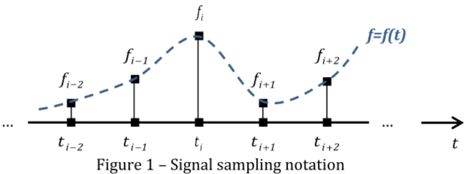
1.1 NOTATIONS i f ∎ f=f(t) 1 i f fi 2 2 i f ∎ fi 1 ∎ ∎ ∎ … ∎ ∎ ∎ ∎ ∎ … 2 i t ti 1 ti ti 1 ti 2 t
Figure 1 – Signal sampling notation
f f(t): continuous time-dependant signal, only known through its measured values at times ti
n n ) n ( dt f d f : nth time-derivative of f
Analysis of some finite difference schemes for slightly noisy time
dependent signals Version : 20/03/15
Laboratoire d'Essai au Feu Page : 5/60
ti i t: sampled time (i is an integer)
t ti ti 1: sample step, or time step (sampling period) fi f(ti): sampled signal, i.e. signal measured at time ti
~
f
i: sampled filtered signal (n)i
f : sampled signal derivative
T d t: differentiation step (d is an integer greater or equal to 1, the case d 1 means that the differentiation step is chosen equal to the sample step, i.e. the step between two consecutive samples).
This document only considers uniformly spaced data, i.e. t doesn’t depend on i, and thus on time.
In some sections below (particularly in the Signal and system approach chapter), the following wordings and notations will equivalently be used:
- “input signal xi” instead of “sampled signal fi”, - “output signal yi” instead of “
f
i~
” or “ (n) i
f ”. 1.2 DEFINITIONS
Very generally, the moving-average filters and the finite difference schemes can be expressed through a linear constant-coefficient equation between their input and output, of the following type:
k k i k i a x y Kernel
The kernel of a scheme refers to the mass function a(k) ak, where k is thus an integer. In practice of course, only a few coefficients ak are nonzero.
In other words, performing such a scheme is equivalent to applying the kernel function to each data point
i
x of the time series. This means that all the samples of the time series are weighted using as weights the values of the kernel function.
Extent
In this document, the extent of a scheme will refer to the collection size of the samples which are encompassed in the scheme. The extent is simply the distance between the two lowest and highest non-zero
k
a .
The extent can equally be expressed as: - a sample number kmax kmin 1, or - a time length tkmax tkmin (kmax kmin) t. 1.3 SUPPORTING EXAMPLE
In order to illustrate the principles developed in this document, the features under study will be illustrated by charts as far as possible.
For this purpose, the signal introduced in Figure 2 will be used as support throughout this document. Each matter under inspection will be exemplified in application to this signal.
Analysis of some finite difference schemes for slightly noisy time
dependent signals Version : 20/03/15
Laboratoire d'Essai au Feu Page : 6/60
Moreover, the first order backward difference with a 1 second differentiation step will be assumed to be the best available approximation of the exact derivative. This will be used as reference for comparison and will appear as light blue underlying curve in the charts when relevant (see Figure 3 for an example).
Analysis of some finite difference schemes for slightly noisy time
dependent signals Version : 20/03/15
Laboratoire d'Essai au Feu Page : 7/60
2 A MATTER OF CHOICES 2.1 TIME SHIFT VS. NOISE FILTERING
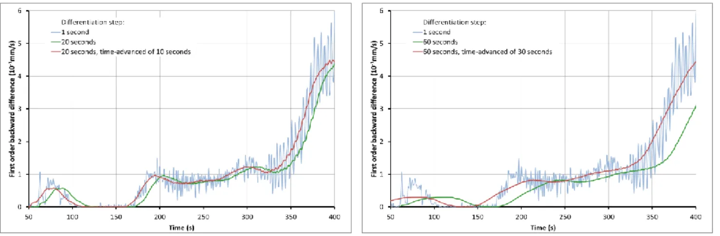
Particularly in the case of experimental data, substantial noise or imprecision may be present in the signal. And here is the crux of the matter: straightforward schemes with short-differentiation steps will amplify this noise, often so much that the result appears to be unusable (Chartrand). Sometimes, talking of noise amplifying is even an understatement: some schemes are affected in a way so sensitive by the high frequency noise in the input signal that they cause it literally to explode.
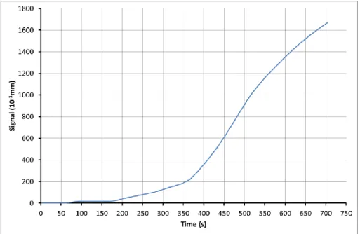
The Figure 2 illustrates real experimental data. The signal consists of deflection measurements – carried out with a position transducer – on a flexural loaded element. The data are acquired at a sampling period of 1 second. Apparently, the signal doesn’t seem affected by any noise. Yet, this is merely an illusion…
Figure 2 – Real experimental data of deflection measurements
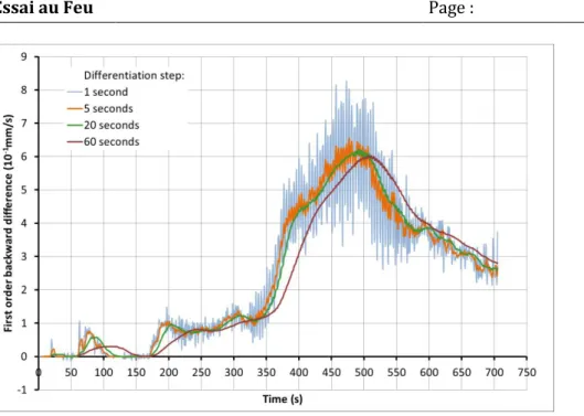
As a first attempt, the differentiation has been processed through a first order backward difference with a 1 second differentiation step (i.e. the step between two consecutive samples). The resulting rate appears in blue curve on Figure 3 below. Its behaviour speaks for itself.
The next attempts make use of the same scheme but with a growing differentiation step (5, 20 and 60 seconds). While increasing the differentiation step has the positive effect of decreasing the noise, it also has two adverse effects: it produces a time shift compared with what would have been expected, and it introduces distortion by broadening and flattening the narrow features. These two negative effects can be summarized in two words: “poor fidelity”.
Analysis of some finite difference schemes for slightly noisy time
dependent signals Version : 20/03/15
Laboratoire d'Essai au Feu Page : 8/60
Figure 3 – Some backward differences attempts
The first lesson is that a compromise should probably be considered between noise reduction, and fidelity. The tools exposed below will help to understand the effect of the involved parameters on these two aspects. Solutions will be investigated to work around the problem by boosting both noise reduction and fidelity. This latter possibility will nevertheless be done at the expense of a truly real-time estimate.
2.2 CAUSALITY VS. NON-CAUSALITY
A system is causal if the output values of the system depend only on the present and the past input values, and do not depend on the future input values. A system is non-causal if its output values depend also on some future input values. Thus, a causal system is non-anticipative, this reflects the common fact that any effect must happen after the cause (Ghosh & Chakraborty, 2010).
In time processing applications, future input values are not yet known and cannot be predicted, real-time systems must thus be causal since they have no choice but to operate on current and past values of the signal (Semmlow, 2012).
However, in the case of off-line processing, i.e. if the data are already stored in a computer, then it is possible to use future signal values along with current and past values to compute an output signal (Semmlow, 2012). Such a situation is common in data processing.
As it will be exemplified in this document, all causal systems give rise to some time delay between their inputs and outputs. Eliminating the time shift inherent in causal systems is the primary motivation for using non-causal systems (Semmlow, 2012).
The second lesson is that a compromise should probably be considered between real-time processing, and eluding time-shift. In the present study, the interest will focus on real-time processing, and thus on causal schemes. Centered schemes – in spite of their non-causal nature – will also be encompassed for the comparison. Nevertheless, the exposed principles still apply for other non-causal schemes.
Analysis of some finite difference schemes for slightly noisy time
dependent signals Version : 20/03/15
Laboratoire d'Essai au Feu Page : 9/60
3 A SHORT PRESENTATION 3.1 MOVING AVERAGE FILTER
3.1.1 Definition
The moving average is the most common low-pass filter, mainly because it is the easiest filter to understand and use. In spite of its simplicity, the moving average filter is optimal for a common task: reducing random noise while retaining a sharp step response. This makes it the premier filter for time domain signals (Smith, 1997).
As the name implies, the moving average filter operates by averaging a number N of points from a raw signal fi to produce each point in the filtered signal
~
f
i. This set of N points forms the kernel of the filter, which is said to be an N-extent filter. In equation form, this is written:1 N 0 j k j i i N f 1 f ~
where k is an integer parameter (Smith, 1997). The common practice limits the values of k to 3 possibilities:
k
0
, backward moving average:N f f ... f f f ~ i (N 1) i (N 2) i 1 i i
k
N
1
, forward moving average:N f f ... f f f ~ i i 1 i (N 2) i (N 1) i 2 1 N
k (if N is odd), centered moving average:
N f ... f ... f f ~ 2 1 N i i 2 1 N i i
The backward moving average makes use of present and past measurements, and is therefore a causal filter. The centered and forward moving averages make use of additional future measurements, and are therefore non-causal filters.
3.1.2 Observations
The backward moving average produces a relative time shift between the filtered signal and the raw signal, leading to a delayed estimation of the signal. On the contrary, the centered moving average doesn’t produce any significant time shift. This backward delay effect occurs as soon as the signal is no longer constant, which is the case when dealing with real signals.
It will be shown that the resulting delay amounts to 2
t ) 1 N
( . In other words, the delay is half the filter extent. One can already easily observe that – if N is odd –
N f ...
fi (N 1) i represents equivalently a
backward moving average in ti and a centered moving average in
2 1 N i
t , the first sampled time being delayed by 2 t ) 1 N
real-Analysis of some finite difference schemes for slightly noisy time
dependent signals Version : 20/03/15
Laboratoire d'Essai au Feu Page : 10/60
time, since the so-computed values are known with a lag of
2T compared to the ideal filtered signal (“the calculated value at time t is the one that actually took place at
2 T t ”).
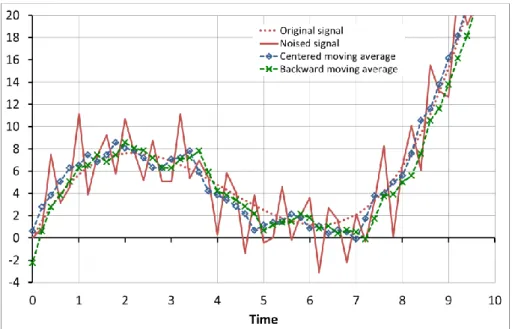
The figures below illustrate the effect of using both methods on a discrete-time signal with a sample step of 0,2 time unit. This signal has been noised by evenly distributed random values.
Figure 4 – Moving average filter with a 3-point extent (the foreseen delay of 0,2 time unit is perceived)
Figure 5 – Moving average filter with an 11-point extent (the foreseen delay of 1 time unit appears clearly)
Analysis of some finite difference schemes for slightly noisy time
dependent signals Version : 20/03/15
Laboratoire d'Essai au Feu Page : 11/60
3.2 FINITE DIFFERENCES
3.2.1 Definition
Any continuous differentiable function f can be expressed into a Taylor series at any point a: ... ) a t ( ! 3 ) a ( f ) a t ( ! 2 ) a ( f ) a t ( ! 1 ) a ( f ) a ( f ) a t ( ! n ) a ( f ) t ( f (1) (2) 2 (3) 3 0 n n ) n (
The application of such Taylor expansion at point ti, using the here considered sampled values, gives:
) T ) T k ( 24 f ) T k ( 6 f ) T k ( 2 f T k f f f (1) i(2) 2 i(3) 3 i(4) 4 5 i i kd i O( For example: T ) 24 T f 6 T f 2 T f T f f f (4) 4 5 i 3 ) 3 ( i 2 ) 2 ( i ) 1 ( i i d i O( T ) 24 T f 6 T f 2 T f T f f f (4) 4 5 i 3 ) 3 ( i 2 ) 2 ( i ) 1 ( i i d i O( T ) 3 T 2 f 3 T 4 f T 2 f T 2 f f f (4) 4 5 i 3 ) 3 ( i 2 ) 2 ( i ) 1 ( i i d 2 i O( T ) 8 T 27 f 2 T 9 f 2 T 9 f T 3 f f f (4) 4 5 i 3 ) 3 ( i 2 ) 2 ( i ) 1 ( i i d 3 i O( …
Appropriate linear combinations of these Taylor expansions give the finite difference formulas and their accuracies. Here are some examples, limited to the ones that will be used further.
First derivatives
backward difference (causal): □ ) T error truncation 4 3 ) 4 ( i 2 ) 3 ( i ) 2 ( i d i i ) 1 ( i 24 T ) T f 6 T f 2 T f T f f f O(
O( (first order scheme)
□ ) T error truncation 4 3 ) 4 ( i 2 ) 3 ( i d 2 i d i i ) 1 ( i 2 ) T 4 T f 3 T f T 2 f f 4 f 3 f O(
O( (second order scheme)
□ ) T error truncation 4 3 ) 4 ( i d 3 i d 2 i d i i ) 1 ( i 3 ) T 4 T f T 6 f 2 f 9 f 18 f 11 f O(
O( (third order scheme)
centered difference (non-causal):
) T error truncation 4 2 ) 3 ( i d i d i ) 1 ( i 2 ) T 6 T f T 2 f f f O(
Analysis of some finite difference schemes for slightly noisy time
dependent signals Version : 20/03/15
Laboratoire d'Essai au Feu Page : 12/60
Second derivatives
backward difference (causal): □ ) T error truncation 3 2 ) 4 ( i ) 3 ( i 2 i 2d d i i ) 2 ( i 12 T ) T 7 f T f T f f 2 f f O(
O( (first order scheme)
Third derivatives
backward difference (causal): □ ) T error truncation 2 ) 4 ( i 3 d 3 i d 2 i d i i ) 3 ( i 2 T ) T 3 f T f f 3 f 3 f f O(
O( (first order scheme)
Note that there is no formal limitation to the possibilities. As an example, asymmetric combination of backward and forward points leads to the uncentered scheme (non-causal):
) T error truncation 4 3 ) 4 ( i d 2 i d i i d i ) 1 ( i 3 ) T 12 T f T 6 f f 6 f 3 f 2 f O(
O( (third order scheme)
The backward difference schemes make use of present and past measurements, and are therefore causal differentiation methods. The centered and forward difference schemes make use of additional future measurements, and are therefore non-causal differentiation methods. The figure below illustrates the effect of using both methods on a piecewise linear signal (f 2t 4 for 2 t 6).
Figure 6 – Comparison of backward and centered difference schemes on a linear signal 3.2.2 Observations
The backward differences produce a relative time shift between the calculated derivative and the exact derivative, leading to a delayed estimation of the derivative. On the contrary, the centered difference doesn’t produce any significant time shift. This backward delay effect occurs as soon as the polynomial order of the signal is greater than the difference scheme order (a quadratic signal for a first order scheme is an example), which is the case when dealing with real signals.
It will be shown that the resulting delay for the first order backward scheme amounts to 2
T . In other words, the delay is half the differentiation step. One can already easily observe that
t k 2
f
Analysis of some finite difference schemes for slightly noisy time
dependent signals Version : 20/03/15
Laboratoire d'Essai au Feu Page : 13/60
equivalently a backward difference in ti and a centered difference in ti k, the first sampled time being delayed by
2 T t
k from the second one. As a consequence, the calculated derivative cannot be known in real-time, since the so-computed values are known with a lag of
2T compared to the exact derivative (“the calculated value at time t is the one that actually took place at
2 T t ”).
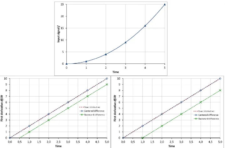
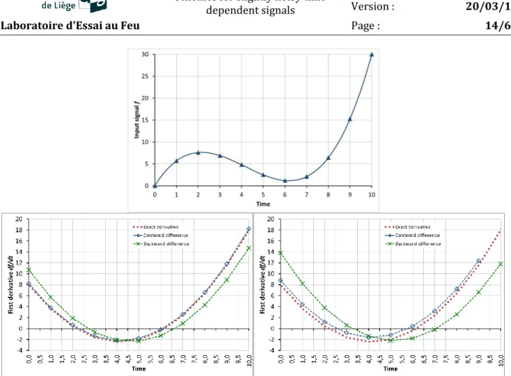
The figures below illustrate the effect of using both methods on two examples (a quadratic signal f t2, a cubic signal f 0,2t3 2,5t2 8t , and a real-life signal) with a sample step of 1 time unit.
Figure 7 – Comparison of backward and centered difference schemes on a quadratic signal Left: differentiation step of 1 time unit (d 1) Right: differentiation step of 2 time units (d 2) (the foreseen delay of 0,5 time unit appears clearly) (the foreseen delay of 1 time unit appears clearly)
Analysis of some finite difference schemes for slightly noisy time
dependent signals Version : 20/03/15
Laboratoire d'Essai au Feu Page : 14/60
Figure 8 – Comparison of backward and centered difference schemes on a cubic signal
Left: differentiation step of 1 time unit (d 1) Right: differentiation step of 2 time units (d 2) (the foreseen delay of 0,5 time unit appears clearly) (the foreseen delay of 1 time unit appears clearly) Finally, the chart below compares backward difference schemes of 1st, 2nd and 3rd orders. The time-shift effect seems to reduce when the scheme order increases, at the expense of a less efficient noise filtering and the occurrence of a specific kind of distortion. This behaviour will be demonstrated below.
Analysis of some finite difference schemes for slightly noisy time
dependent signals Version : 20/03/15
Laboratoire d'Essai au Feu Page : 15/60
3.2.3 A notable property
Applying the first order backward difference of a given discrete-time signal by using consecutive data points (differentiation step chosen equal to the sample step, d 1) gives the rate of the signal at each sampled point i by:
t f f f(1) i i 1
i
These values could then be passed through a backward moving average filter. An N-point extent filter gives the filtered rate of the signal at each sampled point i by:
t N f f t f f N 1 f N 1 f ~ N 1 i i N 0 j 1 j i j i 1 N 0 j ) 1 ( j i ) 1 ( i
In other words, applying an N-differentiation step first order backward difference ( T N t) is equivalent to applying successively an N-extent backward moving average filter on a one-differentiation step first order backward difference ( T t).
As a matter of fact, this example can be generalized: all schemes with multiple-differentiation steps implicitly incorporate a low-pass filtering effect. This will be exemplified below.
Analysis of some finite difference schemes for slightly noisy time
dependent signals Version : 20/03/15
Laboratoire d'Essai au Feu Page : 16/60
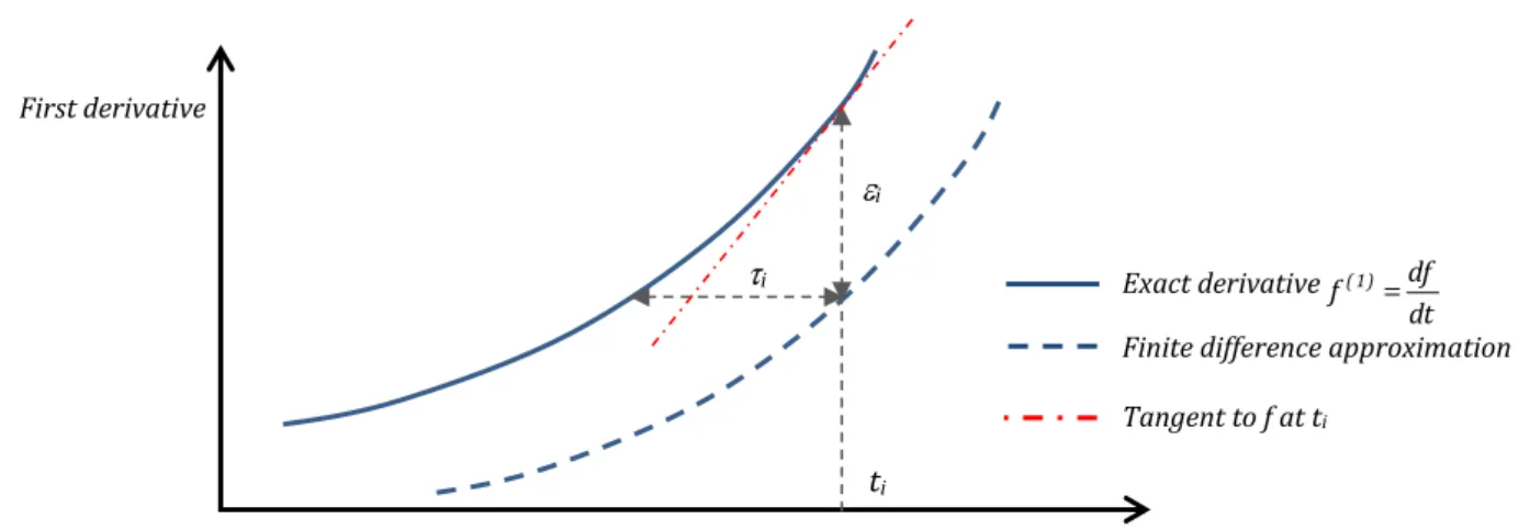
First derivative Time t i ti i Exact derivative dt df f(1)
Finite difference approximation Tangent to f at ti
4 GRAPHICAL APPROACH
Figure 10 – Graphical approach
Denoting by i the truncation error of the considered finite difference scheme at point ti, and by i the associated numerical time delay, this latter delay can be evaluated by the following approximation:
) 2 ( i i i f
A negative delay ( i 0) means that the finite difference approximation is time-advanced compared to the exact derivative, while a positive delay ( i 0) means that the finite difference approximation is time-delayed.
The application of this approximation to the first derivative schemes exposed above gives the delays below: backward difference: □ T ) 24 T f f 6 T f f 2 T 3 4 ) 2 ( i ) 4 ( i 2 ) 2 ( i ) 3 ( i
i O( (first order scheme)
□ T ) 4 T f f 3 T f f 3 4 ) 2 ( i ) 4 ( i 2 ) 2 ( i ) 3 ( i
i O( (second order scheme)
□ T ) 4 T f f 3 4 ) 2 ( i ) 4 ( i
i O( (third order scheme)
centered difference: □ T ) 6 T f f 2 4 ) 2 ( i ) 3 ( i
i O( (second order scheme)
Actually, one should realize that these evaluations of i are only estimations based on a linearized approximation using the tangent to f at ti. As a consequence, the resulting error of this approximation affects the terms in Tn of orders n 1. In other words, only the first term of the first order scheme above
makes sense; all other terms are affected by that error, in such a way that they no longer mean anything and thus prove impossible to interpret.
For this reason, the analysis will now focus on the only relevant relation
2 T
Analysis of some finite difference schemes for slightly noisy time
dependent signals Version : 20/03/15
Laboratoire d'Essai au Feu Page : 17/60
The first order backward difference scheme appears to be mainly biased by a constant shift, amounting to 2T . This first order time-error is ever positive, meaning that this scheme always time-delays the calculated derivative. Systematically shift the calculated derivative by this constant value is the smartest correction that can be made, and it should be done! In practice, this is done by subtracting
2T from the discrete time values. The efficiency on this first order correction is illustrated below on two examples.
Figure 11 – First order backward scheme with first order correction
The same reasoning can be carried out for higher derivatives. For example, the time delay for the first order second derivative is evaluated by:
) 3 ( i i i f
and leads to:
T
i
The analysis then follows as above. The first order backward difference scheme appears to be mainly biased by a constant shift, amounting to
T
. This first order time-error is ever positive, meaning that this scheme always time-delays the calculated derivative.Analysis of some finite difference schemes for slightly noisy time
dependent signals Version : 20/03/15
Laboratoire d'Essai au Feu Page : 18/60
5 SIGNAL AND SYSTEM APPROACH 5.1 TIME DOMAIN
A signal is a description of how one parameter varies with another parameter. A system is any process that produces an output signal in response to an input signal (Smith, 1997). As the present study deals with sampled signals, only will be considered here discrete systems and discrete-time signals.
Example:
The measured deflection fi f(ti) is a discrete-time signal. The first derivative backward difference
T f f f(1) i i d
i is a system that produces a rate of
deflection (output signal fi(1)) from a deflection (input signal fi).
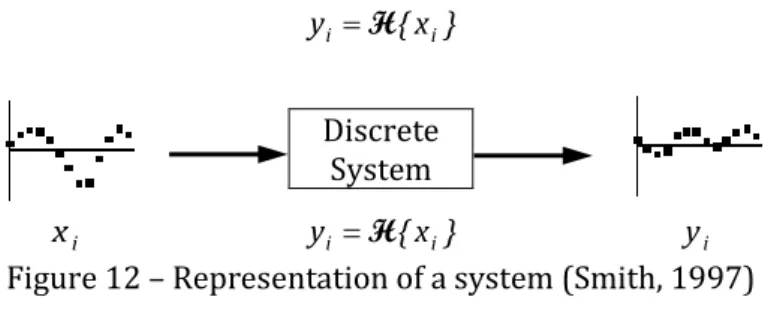
Any system can be described by an operator H which transforms an input sequence into an output sequence: } x { yi H i Discrete System i x yi H{xi} yi
Figure 12 – Representation of a system (Smith, 1997) Defining the unit impulse as the delta function
0 i 0 0 i 1 i
then any signal can be expressed as a linear combination of suitably weighed and shifted impulses. In this case, the weights are nothing but the signal values themselves (Prandoni & Vetterli, 2008). This is called the impulse decomposition: k k i k i x x
The impulse response hi of a system is the signal that exits the system when a delta function (unit impulse) is the input (Smith, 1997):
} { hi H i LTI systems A system is linear if } x { b } x { a } x b x {a 1i, 2i, H 1i, H 2i, H
for any two sequences x1i, and x2i, any two scalars a, b. A system is time-invariant if } x { y } x { yi H i i k H i k
Analysis of some finite difference schemes for slightly noisy time
dependent signals Version : 20/03/15
Laboratoire d'Essai au Feu Page : 19/60
This time-invariance is important because it means that the characteristics of the system do not change with time (or whatever the input signal happens to be). In other words, if a “blip” in the input causes a “blop” in the output, then another “blip” at any other time will cause an identical “blop” (Smith, 1997). When linearity and time-invariance a met simultaneously, the system is said to be a linear time-invariant system, more commonly referred as LTI. These two properties taken together have an incredibly powerful consequence on a system’s behaviour. Indeed, an LTI system turns out to be completely characterized by its impulse response hi: this is all one needs to know to determine the system’s output for any input signal (Prandoni & Vetterli, 2008). In other words, knowing its impulse response hi means knowing everything about the system. This immediately follows from the here above definitions and properties that allow expressing the output of an LTI system as:
k k i k i x h y
where the impulse response hi is invariant and thus unique. Such summation is nothing but the well-known convolution sum of xi and hi and is denoted by the operator *, so that the above relation can be shorthanded to:
i i i x *h
y
The way of understanding how an LTI system changes an input signal into an output signal can be stated as follows. First, the input signal can be decomposed into a set of impulses, each of which can be viewed as a scaled and shifted delta function. Second, the output resulting from each impulse is a scaled and shifted version of the impulse response. Third, the overall output signal can be found by adding these scaled and shifted impulse responses (Smith, 1997).
5.2 FREQUENCY DOMAIN
Fourier analysis is a family of mathematical techniques, all based on decomposing signals into sinusoids and cosinusoids and thus revealing the frequency spectrum of the signals. The signals that can be encountered in the present study are aperiodic discrete type (signals only defined at discrete points between positive and negative infinity, and do not repeat themselves in a periodic sequence). Amongst the different types of Fourier transform, the Discrete-Time Fourier Transform (DTFT) is the one used for such signal type (Smith, 1997).
5.2.1 Definition
The complex DTFT transform X F{xi} changes an input signal xi into an output signal X (the
frequency spectrum of the input signal) through the decomposition equation (Mandal & Asif, 2007):
i i j ie x X
where ejx cos(x) jsin(x) (Euler’s relation) and j 1. The DTFT decomposes the time domain signal into the frequency domain signal, this one containing the amplitudes and the frequencies of the frequency spectrum (component sine and cosine waves) (Smith, 1997).
Inversely, the inverse DTFT transform xi F-1{X } changes an input signal X into an output signal
i
x through the synthesis equation (Mandal & Asif, 2007):
d e X 2 1 x j i i
Analysis of some finite difference schemes for slightly noisy time
dependent signals Version : 20/03/15
Laboratoire d'Essai au Feu Page : 20/60
The inverse DTFT synthesizes the time domain signal from the frequency domain signal.
In its rectangular form, namely X (X ) j (X ), the complex DTFT can also be written as the combination of a real and an imaginary part.
In its polar form, namely X X ej , the complex DTFT can also be written as the combination of a magnitude and a phase:
) X ( ) X ( X magnitude 2 2 ) X ( ) X ( arctan phase
5.2.2 Some useful properties
It directly follows from its definition that the DTFT is a linear operator.
It directly follows from its definition that the DTFT of a real-valued signal is conjugate-symmetric ) X X ( , resulting in: ) X ( ) X ( (X ) (X ) X X
A fundamental property used in signal processing is that Fourier transform of a convolution sum is equal to the product of the Fourier transform. In other words, the convolution sum in the time domain corresponds to multiplication in the frequency domain. It has been shown above that LTI systems are fully described in the time domain by the convolution sum yi xi*hi. As a consequence, an LTI system can also be fully described in the frequency domain by the product
H . X
Y , where H F{hi} is called the “frequency response” (i.e. the frequency response is the Fourier transform of the impulse response). Both the impulse response and the frequency response contain complete information about the system.
A time domain signal and its associated frequency domain signal form a pair. The literature lists tables of pairs for most encountered common signals (as examples, see (Prandoni & Vetterli, 2008), (Mandal & Asif, 2007), or (Rao Yarlagadda, 2010)). The further use of the impulse decomposition together with the two above properties lead the interest on the particular following pair:
k j k i } e { F
The Fourier equations are conceptual representations of discrete time signals that rely on the notion of dimensionless frequencies . The absence of a physical dimension for time has the happy consequence that all discrete time signal Fourier processing become indifferent to the underlying physical nature of the actual signals. This dimensionless abstraction, however, is a drawback from the point of view of intuition because of usual familiarity with signals in the real world for which time is expressed in seconds and frequency is expressed in Hertz (Prandoni & Vetterli, 2008). The precise, formal link between “real world” dimensional frequency fHz (in Hertz) and “Fourier”
dimensionless frequency is given by:
t 2 fHz
and its related angular frequency Hz by:
t
Analysis of some finite difference schemes for slightly noisy time
dependent signals Version : 20/03/15
Laboratoire d'Essai au Feu Page : 21/60
Remembering that ti i t, the arguments i of Fourier equations become
i Hz
i t t
t i i.e. the well-known physical form.
5.2.3 Exact derivatives in frequency domain
In the framework of the study of the properties of calculated derivatives by the finite difference method, it would be very useful to compare them with the exact derivatives n n
dt ) t ( x
d , where x(t) refers to the
continuous-time signal from which the discrete-time signal xi (under consideration in the present study) has been sampled.
The exact derivative being only defined in the continuous-time space – and not in the discrete-time space – the Continuous-Time Fourier Transform (CTFT) is the relevant Fourier transform to use. Without going into detail, the CTFT can be seen as the limit of the DTFT (Discrete-Time Fourier Transform) when t 0. As the DTFT, the CTFT reveals the frequency spectrum. This full equivalence allows drawing a direct comparison between calculated and exact derivatives in the frequency domain.
The CTFT provides the useful pair
X ) j ( dt ) t ( x d n n n F
The frequency response of an ideal differentiator is thus
n . dif Ideal (j ) H Examples:
The frequency response of the first derivative system is
2 j . dif Ideal j e H
The frequency response of the second derivative system is
j 2 2 . dif Ideal e H
The ideal differentiator has a frequency response that increases with frequency; therefore it greatly amplifies high-frequency noises. In practice, when dealing with noisy signals, one would be readily choose a low-pass differentiator rather than a full-pass one (Luo, Ying, & Bai, 2005).
5.3 LINEAR CONSTANT-COEFFICIENT SCHEMES
The moving-average filters and the finite differences share the interesting property of being LTI systems since their input and output are related through a linear constant-coefficient equation of the following type:
2 1 k k k k i k i a x y whose impulse response is thus:
2 1 k k k k i k i a h
Analysis of some finite difference schemes for slightly noisy time
dependent signals Version : 20/03/15
Laboratoire d'Essai au Feu Page : 22/60
Using the properties of the Fourier operator, the frequency response H F{hi} of such linear constant-coefficient equation can be expressed as:
2 1 k k k k j ke a H APPLICATIONS
Backward moving average on N points
N x x ... x x x N 1 y i (N 1) i (N 2) i 1 i 1 N 0 k k i i In this case: else 0 1 N k 0 N 1 ak The frequency response is:
1 N 0 k k j e N 1 H
The above summation represents a geometric progression series, whose general formula is: 1 1 N N N N n k 1 2 2 1
The frequency response becomes:
j N j e 1 e 1 N 1 H
Using some manipulations and the Euler’s relation for sine
j 2 e e ) x
sin( jx jx leads to:
2 ) 1 N ( j e 2 sin 2 N sin N 1 H
First derivative backward difference (first order scheme) T x x y i i d i In this case: else 0 d k T 1 0 k T 1 ak
The frequency response is:
T e 1
Analysis of some finite difference schemes for slightly noisy time
dependent signals Version : 20/03/15
Laboratoire d'Essai au Feu Page : 23/60
Using some manipulations and the Euler’s relation for sine
j 2 e e ) x
sin( jx jx leads to:
2 ) d ( j e 2 d sin T 2 H
First derivative backward difference (second order scheme)
T 2 x x 4 x 3 y i i d i 2d i In this case: else 0 d 2 k T 2 1 d k T 2 4 0 k T 2 3 ak
The frequency response is:
T 2 e e 4 3 H j d j2 d T )) d cos( 2 )( d sin( j T )) d cos( 1 ( H 2
Using some manipulations and fundamental trigonometric relations leads to:
2 )) d cos( 1 ( )) d cos( 2 )( d sin( arctan j 2 e T 5 ) d cos( 8 ) d ( cos 3 H
First derivative backward difference (third order scheme)
T 6 x 2 x 9 x 18 x 11 y i i d i 2d i 3d i In this case: else 0 d 3 k T 6 2 d 2 k T 6 9 d k T 6 18 0 k T 6 11 ak
The frequency response is:
T 6 e 2 e 9 e 18 11 H j d j2 d j3 d or T 3 )) d ( cos 4 ) d cos( 9 8 )( d sin( j T 3 ) d ( cos 4 ) d ( cos 9 ) d cos( 6 1 H 2 3 2
Analysis of some finite difference schemes for slightly noisy time
dependent signals Version : 20/03/15
Laboratoire d'Essai au Feu Page : 24/60
First derivative centered difference (second order scheme)
T 2 x x y i d i d i In this case: else 0 d k T 2 1 d k T 2 1 ak The frequency response is:
T 2
e e
H j d j d
Using some manipulations and the Euler’s relation for sine
j 2 e e ) x
sin( jx jx leads to:
2 j e ) d sin( T 1 H
Second derivative backward difference (first order scheme)
2 d 2 i d i i i T x x 2 x y In this case: else 0 d 2 k T 1 d k T 2 0 k T 1 a 22 2 k
The frequency response is:
2 d 2 j d j T e e 2 1 H
Using then some manipulations and fundamental trigonometric relations leads to:
) d ( j 2 2 2 e d sin T 4 H 5.4 SPECTRUM ANALYSIS
Let’s resume two main concepts.
An LTI system is fully described in the frequency domain by the product Y X .H . The quantities X and Y are the DTFT of the input and output signals, while the frequency response H is the DTFT of the impulse response of the operator describing the LTI system that produces the output signal in response to the input signal.
A Fourier transform generates a spectrum in the frequency domain – W F{wi} – from a signal or an operator wi. This spectrum – function of – is a complete, alternative representation of the
signal or operator, and the analysis of the spectrum reveals the fundamental information required to characterize and classify the signal or operator in the frequency domain (Prandoni & Vetterli, 2008).
Analysis of some finite difference schemes for slightly noisy time
dependent signals Version : 20/03/15
Laboratoire d'Essai au Feu Page : 25/60
The relation Y X .H highlights the way the frequency response H acts on the input signal: through this simple multiplication, H modulates X into Y . The spectrum analysis of H will thus inform how the LTI system modify the input signal into the output signal at each angular frequency .
Since the transform values are complex numbers, it is customary to separately analyse their magnitude and their phase. As a reminder, the complex frequency response can be written in its polar form H H ej where: ) H ( ) H ( H magnitude 2 2 ) H ( ) H ( arctan phase
The relation between dimensionless and dimensional frequencies
t 2
fHz and angular frequencies
i Hz
i t t
t
i will also be used in the analysis.
Note that in the charts here below, the axes have been made intentionally dimensionless. This choice is more convenient for the analysis.
5.4.1 Magnitude spectrum
From the perspective of the Fourier representation as being a sum of sine and cosine waves, the magnitude spectrum defines the inherent power produced by each of the waves (Prandoni & Vetterli, 2008). The magnitude is thus related to the energy distribution of the operator in the frequency domain. By its “scaling” action, the magnitude
H
of an operator will expand or attenuate the input signal, as a function of . This corresponds to the filtering effect of the operator.According to the way the magnitude spectrum affects the signal, the operator filtering effect can be classified into broad categories (lowpass, highpass, bandpass, … operators).
The frequency interval (or intervals) for which the magnitude of the frequency response is zero (or practically negligible) is called the stopband, or the cuttoff frequency. Conversely, the frequency interval (or intervals) for which the magnitude is non-negligible is called the passband (Prandoni & Vetterli, 2008). In the spectra below, the curve of the frequency response of ideal differentiators (HIdealdif. (j )n) will be
shown for comparison.
APPLICATIONS
Backward moving average on N points
2 sin 2 N sin N 1 H
Analysis of some finite difference schemes for slightly noisy time
dependent signals Version : 20/03/15
Laboratoire d'Essai au Feu Page : 26/60
Figure 13 – Backward moving average with an N-extent
The efficiency of the high frequency attenuation is rather poor, and the stopband is not so clear. The moving average filter cannot effectively separate one band of frequencies from another. But good performance in the time domain results in poor performance in the frequency domain, and vice versa. In short, the moving average should be considered as a very good smoothing filter (the action in the time domain), but a very poor low-pass filter (the action in the frequency domain) (Smith, 1997).
As can be seen, the “smoothing power” of this filter is dependent on the number of samples taken into account in the average or, in other words, on the extent N: the more the filter extent grows, the more the highest frequencies are dampened, and the more the high frequency noise is attenuated. Therein lies the interest of increasing N.
A useful definition of the cuttoff frequency could be the lowest frequency for which
H
0
, i.e. for which2
N . This gives the cuttoff frequency
t N
1
fHz , where N t is the extent of the filter.
First derivative backward difference (first order scheme)
2 d sin T 2 H
The case d 1 means that the differentiation step is chosen equal to the sample step (i.e. the step between two consecutive samples). This choice turns out to amplify the higher frequencies while absorbing the lower ones. This explains why this backward “one step” difference scheme is affected in a way so sensitive by the high frequency noise in the input signal: it causes it literally to explode. On the other side, the more the differentiation step grows, the more the modulation equilibrates at the same level for all the represented frequencies, the more this amplification level decreases, and the more the global noise is attenuated. Therein lies the interest of increasing d.
Analysis of some finite difference schemes for slightly noisy time
dependent signals Version : 20/03/15
Laboratoire d'Essai au Feu Page : 27/60
Anyway, this difference scheme will never wipe off the higher frequencies of the input signal: the frequency range of the input will always remain the same in the output.
The maximum value is
T 2
H max , where T d t. This means that doubling the differentiation step
T
will double the attenuation of the noise magnitude.Figure 14 – First order backward difference with a d-differentiation step First derivative backward difference (second order scheme)
5 ) d cos( 8 ) d ( cos 3 T 1 H 2
The global shape of the curves and their relative proportions are the same as the ones for the backward first order scheme above; so does their interpretation.
The maximum value is
T 4
H max , where T d t. This means that doubling the differentiation step
T
will double the attenuation of the noise magnitude. But this maximum value is also twice the maximum value of the backward first order scheme above. This means that, for a same differentiation stepT
, the backward first order scheme will attenuate the noise magnitude twice as much than the backward second order scheme (see Figure 9 for an example).Analysis of some finite difference schemes for slightly noisy time
dependent signals Version : 20/03/15
Laboratoire d'Essai au Feu Page : 28/60
Figure 15 – Second order backward difference with a d-differentiation step First derivative backward difference (third order scheme)
2 d sin )) d cos( 22 ) d cos( 91 87 ( 2 T 3 1 H 2
Figure 16 – Third order backward difference with a d-differentiation step
The global shape of the curves and their relative proportions are the same as the ones for the backward first and second orders scheme above; so does their interpretation.
The maximum value is
T 3
20
H max , where T d t. This means that doubling the differentiation step
T
will double the attenuation of the noise magnitude. But this maximum value is also 3,33 times the maximum value of the backward first order scheme above. This meansAnalysis of some finite difference schemes for slightly noisy time
dependent signals Version : 20/03/15
Laboratoire d'Essai au Feu Page : 29/60
that, for a same differentiation step
T
, the backward first order scheme will attenuate the noise magnitude 3,33 times as much than the backward third order scheme (see Figure 9 for an example). First derivative centered difference (second order scheme)) d sin( T 1 H
Figure 17 – Second order centered difference with a d-differentiation step A direct observation is that
order 2nd centered order st 1 backward H (d ) ) 2 d ( H . The interpretation
is thus the same as the one for the backward first order scheme, wherein the only even values of d remains, meaning that the worst case “d 1” encountered in this last scheme is avoided here. The maximum value is
T 1
H max , where T d t. This means that doubling the differentiation step
T
will double the attenuation of the noise magnitude. But this maximum value is also half the maximum value of the backward first order scheme above. This means that, for a same differentiation stepT
, the centered second order scheme will attenuate the noise magnitude twice as much than the backward first order scheme.Second derivative backward difference (first order scheme)
2 d sin T 4 H 2 2
Analysis of some finite difference schemes for slightly noisy time
dependent signals Version : 20/03/15
Laboratoire d'Essai au Feu Page : 30/60
Figure 18 – First order backward difference with a d-differentiation step
The case d 1 means that the differentiation step is chosen equal to the sample step (i.e. the step between two consecutive samples). This choice turns out to amplify the higher frequencies while absorbing the lower ones. This explains why this backward “one step” difference scheme is affected in a way so sensitive by the high frequency noise in the input signal: it causes it literally to explode. On the other side, the more the differentiation step grows, the more the modulation equilibrates at the same level for all the represented frequencies, the more this amplification level decreases, and the more the global noise is attenuated. Therein lies the interest of increasing d.
Anyway, this difference scheme will never wipe off the higher frequencies of the input signal: the frequency range of the input will always remain the same in the output.
The maximum value is max 2 T 4
H , where T d t. This means that doubling the differentiation step
T
will quadruple the attenuation of the noise magnitude.5.4.2 Phase spectrum
From the perspective of the Fourier representation as being a sum of sine and cosine waves, the phase spectrum defines the relative alignment of the waves. While this does not influence the energy distribution in frequency, this phase alignment does have a significant effect on the shape in the time domain (Prandoni & Vetterli, 2008). By its “shifting” action, the phase of an operator will delay or advance the input signal in the time domain, as a function of . This corresponds to the distortion and time shift effects of the operator. Remembering
the definition of the DTFT
i i j ie x X ,
the frequency domain description of an LTI system Y X .H , and the polar form of the frequency response H H ej ,
Analysis of some finite difference schemes for slightly noisy time
dependent signals Version : 20/03/15
Laboratoire d'Essai au Feu Page : 31/60
it follows i ) i ( j ie x H Y
The dimensionless parameter ( ) is called the “phase delay” of the system, and is a function of frequency. Using the relation between dimensionless and dimensional angular frequencies
i Hz
i t t
t
i , the argument of the wave components becomes Hz(ti ). It appears now clearly that the dimensional form of the phase delay ( ) t – where is the phase of the frequency response of the system – gives the time delay experienced by each wave component of a signal through the system.
The interpretation is as follows:
- when the phase experiences negative values, the phase delay is positive, meaning that the operator delays the input signal (i.e. shift it to the right in the time domain),
- when the phase experiences positive values, the phase delay is negative, meaning that the operator advances the input signal (i.e. shift it to the left in the time domain).
Quite generally, the phase of the operator will be different for the various frequencies, so does the phase delay. This delay variation means that signals consisting of multiple frequency wave components will undergo distortion because these wave components are not shifted by the same amount of time at the output of the system. This phenomenon changes the shape of the output signal compared to the expected one. Sufficiently large delay variation can cause problems such as poor fidelity of the system (Pinki & Mehra, 2014).
In contrast, if the phase of the operator is linear (in ) within its passband, then the phase will shift all the wave components of the input signal as a single block. Such linear phase operator is said to be “distortionless”.
The present purpose is to determine the time shift resulting of the use of a time-discrete scheme instead of the related ideal system. The phase delay of the system is then the relevant parameter. One need only compare the phase delay of the scheme under study with the phase delay of the related ideal system. Two situations will be encountered here.
1. Filters that are only dedicated to noise elimination are not intended to change the basic shape of signals to which they apply. This feature is precisely one of the main ones that could be expected from a filter. In this first case, the output signal must simply be compared with the input signal, and the time shift produced by the system is given by the phase delay of the system.
2. Derivatives of signals, on the contrary, fall into the category of systems that change significantly the shape of signals to which they apply, and also their nature (this may in fact be the reason why the systems of this category are being designed and used). In this case, the only phase delay of the system describes a delay measurement that becomes somewhat arbitrary and meaningless. Comparing the output signal with the input signal doesn’t make sense anymore. Finite difference schemes must be compared with their related ideal differentiator. Hence, the time shift produced by the system is:
t 2 Scheme . dif Ideal
Scheme for first derivatives,
Analysis of some finite difference schemes for slightly noisy time
dependent signals Version : 20/03/15
Laboratoire d'Essai au Feu Page : 32/60
…
In other words, the quantity ( ) is nothing but the numerical time delay i – defined in the above graphical approach – decomposed as a function of the frequency.
Unwrapping step
Before introducing the detailed phase spectra, the attention must be drawn on a subtle handling that must be performed when computing the phase. This processing is called “phase unwrapping” (Smith, 1997). The phase has been defined as
) H ( ) H (
arctan . Using any software to compute the arctangent will generate a chopped signal, as can be seen on Figure 19 (raw phase curve). The apparent discontinuities in the signal are a result of the computer algorithms picking their favorite choices from an infinite number of equivalent possibilities. The smallest possible value is always chosen, keeping the phase in the range
2
to
2 .
Actually, there is no mathematic reason why the phase should be limited in this range. The understanding of the phase therefore requires first to remove these discontinuities, even if it means that the phase extends above
2 or below 2 . This unwrapping step shall be performed following the two successive handling:
1. if both the real and imaginary parts are negative, subtract radians from the calculated phase; if the real part is negative and the imaginary part is positive, add radians;
2. add or subtract integer multiplies of 2 from each sample, where the integer is chosen to minimize the discontinuities between successive points, as can be seen on Figure 20.
Analysis of some finite difference schemes for slightly noisy time
dependent signals Version : 20/03/15
Laboratoire d'Essai au Feu Page : 33/60
APPLICATIONS
Backward moving average on N points
t 2 ) 1 N ( 2 ) 1 N (
The backward moving average on N points generates a positive delay independent of the frequency. The average calculated by this filter is thus shifted half of the extent of the filter to the right in the time domain. This means that doubling the extent of the filter N will double the delay. Since the time shift is independent of the frequency , no distortion is introduced.
First derivative backward difference (first order scheme)
t 2 ) d ( 2 ) d ( and 2 T t 2 d
where T d t. The backward first order scheme generates a positive delay independent of the frequency. The derivative calculated by this difference scheme is thus shifted half of the differentiation step to the right in the time domain. This means that doubling the differentiation step
T
will double the delay. Since the time shift is independent of the frequency , no distortion is introduced.First derivative backward difference (second order scheme)
2 2 (1 cos( d)) )) d cos( 2 )( d sin( arctan t )) d cos( 1 ( )) d cos( 2 )( d sin( arctan and t )) d cos( 1 ( )) d cos( 2 )( d sin( arctan 2 2