3-D density imaging with muon flux measurements from
underground galleries
N. Lesparre,1,2,* J. Cabrera1and J. Marteau3
1 IRSN, B.P 17, F-92262 Fontenay-aux-Roses Cedex, France.
2OREME, Géosciences Montpellier (UMR CNRS 5569), Université Montpellier, F-34095 Montpellier Cedex 5, France 3IPNL (UMR CNRS-IN2P3 5822), Université Lyon 1, Lyon, France
KEYWORDS: Inverse theory; Tomography; Fractures and faults; High strain deformation zones.
ABSTRACT
Atmospheric muon flux measurements provide information on subsurface density distribution. In this study, muon flux was measured underground, in the Tournemire experimental platform (France). The objective was to image the medium between the galleries and the surface and evaluate the feasibility to detect the presence of discontinuities, for example, produced by secondary subvertical faults or by karstic networks. Measurements were performed from three different sites with a partial overlap of muon trajectories, offering the possibility to seek density variations at different depths. The conversion of the measured muon flux to average density values showed global variations further analysed through a 3-D nonlinear inversion procedure. Main results are the presence of a very low density region at the level of the upper aquifer, compatible with the presence of a karstic network hosting local cavities, and the absence of secondary faults. We discuss the validity of the present results and propose different strategies to improve the accuracy of such measurements and analysis.
1.
INTRODUCTION
France, Belgium, Switzerland and the Netherlands planned to store nuclear waste in deep underground geological disposal in a clayey medium. Some clayey rocks present properties such as a very low hydraulic conductivity favouring the retention of radionuclide in the hosting medium that acts as a barrier and limits the propagation of radioactive elements to the biosphere (Leroy et al. 2007; Yven et al. 2007). However the confining properties of the clayey medium might differ in zones affected by tectonic faults. Such perturbations are likely to increase the permeability of the hosting rock, thus affecting its confining role (Gelis et al. 2015). Thus, the assessment of faults zones at the vicinity of a storage site is of prime importance. In such a context, geophysical methods supply useful information to detect and characterize discontinuities produced by the fault displacement. Nevertheless subvertical faults with small vertical displacements remain hard to distinguish. Geophysical images showing an unperturbed medium have to be interpreted with caution, as discontinuities could remain invisible depending on the method used, its resolution and penetration depth.
The fractured medium in rocks such as limestones is likely to present a higher macroporosity compared to unperturbed regions. Gravimetric methods could be suitable to detect and characterize faults by showing lower density regions, however the method suffers from a strong non-uniqueness
and low-resolution performances (Li & Oldenburg 1998; Calcagno et al. 2008; Guillen et al. 2008). In contrast, recent studies show the interest of muon flux measurements to obtain density images with a better resolution and a reduced non-uniqueness of the inverse problem (Tanaka et al. 2005; Lesparre et al. 2010; Tanaka et al. 2010). Actually, muon flux measurements complement fruitfully gravity data for constructing high-resolution images (Davis & Oldenburg et al. 2012; Nishiyama et al. 2014; Jourde et al. 2015). Muons produced in the atmosphere can travel through a few kilometres from the surface, with an attenuation that depends on the medium density and on the travelled length. So by knowing the trajectory of the detected muons, it is possible to deduce the medium density. The method was first applied to sound the Kephren pyramid (Alvarez et al. 1970). Further technological developments allowed the application of the method for imaging volcanoes (Tanakaetal. 2005; Lesparre etal. 2012c; Portaletal. 2013; Carbone et al. 2014; Nishiyama et al. 2014; Jourde et al. 2015). Recently the method was used for localizing the uranium dioxide fuel in a reactor of the Fukushima Daiichi nuclear power plant (Sugita et al. 2014). The interest of the method for mining exploitation was also tested (Bryman et al. 2015).
First applications analysing the muon flux crossing a geological target showed images produced from one site of muon flux detection. In the various studies, the extraction of information about the medium heterogeneity has been performed with different types of muon flux conversions.
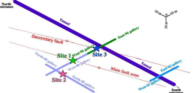
Figure 1. Tournemire experimental platform with the main tunnel and the experimental galleries. The locations of the different sites of acquisition are indicated by the stars.
Ambrosino et al. (2015) show the number of events detected in the different angles of view of the sensor, while Carloganu et al. (2013) and Portal et al. (2013) display the muon flux absorption by the studied object. Such types of data conversions are dependent on the thickness crossed by muons along the different sensor angles of view. Carbone et al. (2014) represent a normalized difference between simulated and measured muon flux. Finally, Tanaka et al. (2005) and Lesparre et al. (2012c) present density radiographies of the probed object, that correspond to the average density values estimated along each telescope angles of view. The reconstruction of the medium density distribution would have required data measured from at least two acquisition sites with crossing angles of view.
A 3-D density model was obtained with data measured from two sites, either using a linear regularized inversion (Tanaka et al. 2010), or with a nonlinear inversion seeking discrete density values (Jourde 2015). The difficulty of imaging objects of thickness higher than 800 m was highlighted, notably with sensors exposed to the open sky muon flux, as this is generally the case, when imaging volcanoes since upward-going muons add noise to the signal coming from the target (Lesparre et al. 2012c; Jourde et al. 2013; Ambrosino et al. 2015).
For this study, a muon detector (later called the telescope) is placed in underground galleries of the Tournemire experimental platform at three different locations known to be representative of media perturbed or unperturbed by faults. Thus, the chosen configuration allows the crossing of some of the detected muon trajectories, supplying information to reconstruct the density distribution at different depths from the galleries to the surface. Estimated average density values show the presence of a low density region above the acquisition site coinciding with a fault zone observed on the gallery walls. We apply a nonlinear inversion scheme based on the simulated annealing method to the muon flux data in order to construct a 3-D density image. Such a methodology provides the density distribution of the medium above galleries together with an estimate of the density error distribution, thus giving an idea on the observed targets reliability. The 3-D image interpretation is sustained by geological information.
2.
CONTEXT OF THE EXPERIMENT
2.1.
GEOLOGICAL CONTEXT
The experimental platform of Tournemire (Aveyron, France) is composed of a main tunnel from which experimental galleries were excavated (Fig. 1). The platform is located in a sedimentary monocline structure dipping to the north (4-5 ; Fig. 2). The tunnel is located in the Toarcian layer made of well-compacted and thinly bedded claystones and marls (Matray et al. 2007). Above, the Aalenian, Bajocian and Bathonian are limestone layers (Fig. 2). The transition from the Toarcian to the Aalenian is progressive. The Aalenian marks the beginning of carbonated deposits from the Jurassic, its upper part shows a more massive composition (Cabrera et al. 2001). The Bajocian and Bathonian layers are made of massive limestones and dolomites.
The Toarcian is overlaid by an upper aquifer intercepted by upward boreholes drilled from the tunnel and reaching the bottom part of the Aalenian. This aquifer flows from south to north and follows the geological layer dip (Fig. 2). Fluid flows might locally form karstic structures along mainly N-S fractured zones. The aquifer presents an outlet in the tunnel, close to the regional Cernon fault that delimits the southern block at a distance of about 1600 m from the tunnel south entrance (Fig. 2). The Cernon fault is an old Paleozoic E-W major crustal discontinuity reactivated during the Jurassic extension and later by the compressional Pyrenean tectonic (Cabrera et al. 2001; Constantin et al. 2004; Lesparre et al. 2016). The Cernon fault length is about 80 km, and connects a northern block of fractured dolomitic rocks from the Hettangian. Several secondary N-S fault zones are also observed in the experimental galleries. They correspond to strike-slip displacements produced or reactivated during the Pyrenean compression (Cabrera et al. 2001; Constantin et al. 2004). Their extension is of a few kilometres and they present a fault gouge of about 1 m wide or breccias of 10-20 m (Gelis et al. 2015).
2.2.
INSIGHTS FROM PREVIOUS GEOPHYSICAL EXPERIMENTS
The IRSN explored at Tournemire the potential of different geophysical methods to detect and characterize discontinuities related to small vertical displacements either by surface or by underground experiments. A 3-D high-resolution seismic experiment showed discontinuities due to secondary faults below the clay layers, where displacements were most important. However, in the clay layer and in the limestone layers above, the displacements affecting the reflection surfaces were too small to be clearly distinguished on the resulting image (Cabrera 2005). A second seismic experiment was performed from the galleries South-08 and West-08 in order to supply local information on the secondary fault structures (Bretaudeau et al. 2013). The resulting images are defined in a horizontal plane, roughly parallel to the stratification, at the tunnel elevation. They show that the two secondary faults observed on gallery walls are connected by a complex network of fractures.
Electrical resistivity tomographies were also performed from the surface, above the experimental galleries. A first experiment consisted in the acquisition of two E-W profiles and a N-S one of more than 2 km, with inter-electrode distance of 40 m (Gelis et al. 2010). Three faults zones were observed on the E-W images but due to the large distance between electrodes, their locations were inaccurate. The upper limestone layers showed to be highly heterogeneous, that was interpreted by spatial variations of the medium degree of fracturation. The clay layer was identified as a highly conductive medium in agreement with measurements on samples from the experimental galleries performed by Cosenza et al. (2007). However there was no evidence on the resistivity image of the secondary faults crossing that conductive homogeneous region. The high resistive contrast between the clay and the limestone upper layers as well as the important depth of the clay layer (about 200 m below surface) prevented the detection of discontinuities in the clay medium. A second experiment was performed with a higher resolution by reducing the inter-electrode distance to 2, 4 and 8 m, which implied also a reduction on the investigation depth to a hundred of meters (Gelis et al. 2015). The images confirmed the presence of subvertical conductive structures, correlated with fractured rocks observed at surface. Finally, induced polarization measurements were also performed from the galleries (Okay et al. 2013). Their analysis allowed distinguishing between recent fractures created during galleries excavation from cracks of older origin that were filled with calcite containing pyrite, which induced chargeability anomalies.
2.3.
INFORMATION ON THE MEDIUM DENSITY
Concerning the estimate of the density variations in the different rock layers of regions perturbed or not by secondary faults, only a few measurements were performed on samples from vertical boreholes drilled from the tunnel to the first metres of the Aalenian layer (Matray et al. 2007). Samples from the clay medium showed a density of about 2.6 g cm-3 while limestone samples showed a density
of about 2.65 g cm-3. During our experiment new boreholes were drilled from the gallery walls in
perturbed and unperturbed zones. Sample analyses showed average densities of about 2.55 g cm-3
and 2.65 g cm-3 in the perturbed and unperturbed media, respectively.
The density values obtained from sample analyses are used to constrain the inversion that aims at reconstructing the density image distribution. Density values do not show strong variations in the clay medium affected by faults neither high contrasts between the clay and limestone materials. We rather seek for density contrasts in the limestone medium that could produce a macroporosity and thus a low density region at the level of the faults zones, while density in the massive dolomites of the Bajocian and Bathonian might be as high as 2.85 g cm-3. The Larzac plateau is also known to host
karstic networks that present, in some places, important cavities with dimensions of a few tens of metres. The development of karsts is controlled by the presence of structures in the medium such as the bedding or tectonic faults (Bakalowicz 2005). The low permeability of the clay layer favours a horizontal flow of the water in the Aalenian layer located just above and where conduits and cavities could be encountered (Figs 2 and 3). The presence of such structures would create anomalies of low density on the image.
3.
DENSITY IMAGING FROM MUON FLUX
3.1. MUON FLUX PREDICTION
Muons are charged particles of the lepton family presenting a rest mass of 105 MeV and produced in atmospheric cosmic ray showers. Muon sensors have to be placed below the object, for instance beneath a mount or in an underground gallery to detect atmospheric muons and probe the medium above the sensor.
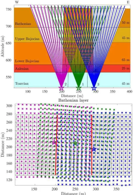
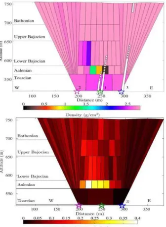
Figure 3. Cross-section of the Tournemire range in the W-E direction. The coloured straight lines show the region sounded from each site. The red hashed lines indicate the faults as observed from the galleries with an interpretation on the geometry of their prolongation.
The muon flux can be estimated from the knowledge of the probed rock opacity Q, that is, the rock density p integrated over the length L of the muon paths in the medium:
The opacity corresponds to the quantity of matter crossed by muons and is equivalent to the multiplication of the total length crossed L with the medium average density along L.
The muon flux is filtered as muons are crossing the medium since for a given opacity muons presenting an energy lower than Emin(Q) are absorbed (Groom et al. 2001). The total underground
muon flux ϴ corresponds to the integration of the muon flux spectra at surface Øsurf between Emin (Q)
and the infinite:
is expressed in cm-2 sr-1 s-1. Ø
surf depends on the zenith angle Ø of the muon trajectories and on
the muon initial energy E, that is, the muon kinetic energy when produced from its parents decay (Gaisser 1990). In this paper we simulate the underground muon flux using a model of the atmospheric muon flux attenuated when crossing matter Tang et al. (2006). The muon minimum energy for crossing a given opacity is estimated using attenuation constants given by the particle data group tables (Olive et al. 2014).
3.2.
MUON SENSORS
The muon detector, the so-called ‘telescope’, is made of three detection matrices, each containing Nx
through ionization with the scintillating strips and their trajectories are determined by the pairs of fired pixels (aij, cmn). aij and cmn refer to the pixels of the front and rear matrix respectively. The
combination of pixels from the front and rear matrices constitutes a set of (2Nx — 1) x (2Ny — 1)
telescope angles of view rop with o = i — m and p = j — n. The angles of view depend only on the relative
shift between the aij and cmn pixels (Lesparre et al. 2012a; Marteau et al. 2012; Jourde et al. 2013). The
third matrix in the middle is used to filter the signal and reject backgrounds and random coincidences. Only events with a triple coincidence and pixels aligned along a straight trajectory are considered as muon signal candidates (Lesparre et al. 2012c). The number of detected muons v for the different rop
directions depends on the telescope acceptance expressed in cm2 sr and on the data
recording duration reflects the telescope sensitivity to muons coming from a given direction in a given solid angle (Lesparre et al. 2012b)
Sop, the detection surface in a given direction, depends on the pixels size d and on the number of pixels
Nx x Ny of each matrix. The solid angle depends on the inter-matrix distance D that thereby
de-termines the resolution of the lines of sight. The closer the matrices are, the higher the solid angle is. The choice of the distance between matrices depends on the spatial resolution required to probe a given target in the medium (Lesparre et al. 2010). The acceptance is maximal in the r00
direction, perpendicular to the matrices, since all pixels contribute to the detection surface. The smallest acceptance values correspond to directions that most depart from r00 since only a few pixels
contribute to the detection. Therefore, only the flux coming from a fraction of all possible detection directions is analysed in the following.
In the present experiment the number of scintillator bars in each direction is Nx = Ny = 16 defining
detection pixels of 5 cm x 5 cm (Lesparre et al. 2012a; Marteau et al. 2012). There are 31 x 31 = 961 detection directions rop. Each scintillating bar being 0.8 m long, the total detection surface of a matrix
is 0.64 m2. The distance between the front and rear matrices is set to D = 120 cm for all acquisitions.
The maximal theoretical acceptance in this configuration is 11 cm2 sr. However, since the acceptance
decreases quickly for angles of view away from the telescope main direction r00, data acquired for the
most extreme angles of view are not considered in the analysis because they present low statistics. More precisely, the six most extreme lines of sight are removed, leaving 19 x 19 = 361 detection directions in the data sample. So the selected telescope angles of view correspond to rop with o and p
varying in the range [-9; 9].
3.3.
MEASURED MUON FLUX
Since the different sources of noise on the muon flux are independent, the estimate of the measured muon flux error writes:
We assume that muons crossing the telescope follow a Poissonian distribution with parameter y, corresponding to the number of events detected per day (Gaisser 1990). The average number of muons detected per day presents a noise with a 95 per cent confidence interval of
, where is the number of acquisition days. The noise related to the telescope acceptance is evaluated to be less than 3 per cent (see Lesparre et al. 2012b). The noise on the duration of the acquisition is estimated to be less than 2 per cent. A careful evaluation of the readout dead times was performed since they may decrease the overall detection efficiency (for a detailed description of the procedure, see Marteau et al. 2014). Thus, the noise affecting the measured muon flux is mainly induced by its random nature. In the following, the selected data present a muon flux error lower than 25 per cent.
4.
FIELD EXPERIMENT
4.1. Measurement setup
For the reconstruction of the density images, the telescope was placed at three consecutive locations in the underground galleries of the Tournemire experimental platform to image the medium from the galleries to surface (Fig. 1). Sites 1 and 3 correspond to fractured regions observed on the gallery walls, while site 2 coincides with an unperturbed region since no fracturation is noted on the gallery walls (Fig. 3). The orientation of the telescope and the duration of acquisition at each site are summarized in Table 1.
In perturbed regions, the medium is fractured over distances of about 10 mas observed on gallery walls. The telescope is configured so its angles of view are distant from each other by about 10 m at the surface level. The rock thickness above the telescope is about 230 m for each acquisition site (Table 1). The aperture angle in the main direction r00 of the telescope is of 6° so the area explored at surface by this angle of view is about 400 m2.
Table 1. Configuration of the telescope at each site of acquisition. Dmatriœs corresponds to the distance between
extreme matrices. The thickness, muon flux, opacity and average density values are given for the angle of view in the main direction of the telescope.
4.2. MUON FLUX DATA TO AVERAGE DENSITY ESTIMATE
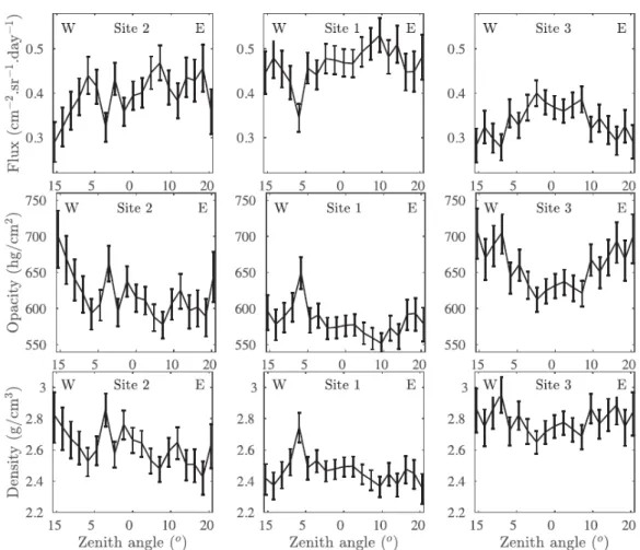
The muon flux detected from site 1 is globally significantly higher than the one detected from sites 2 and 3 (Fig. 4 and Table 1). The muon flux model of (Tang et al. 2006) is used in order to compute tables of opacity . Then, the medium opacity p is deduced from the measured muon flux. The error of the opacity is given by
since Q decreases with increasing values of . The opacity shows an opposite variation from the muon flux since the muon flux decreases while the opacity increases. Thus, the opacity estimated from site 1 measurements presents lower values than the one estimated from sites 2 and 3 (Fig. 4 and Table 1).
The average medium density the muon paths is obtained from the ratio between the estimated opacity and the total distance L travelled by muons across the medium. The sources of noise on the density are independent since they are related to the noise affecting the opacity and to the error on the rock thickness. From equation 1, the noise of the average density is evaluated by:
with L the thickness of rock crossed by muons and its associated error presents a contribution of about 20 per cent of the noise affecting the average density.
The average density above the galleries shows a reduced value at site 1 of 2.49 ± 0.07 g cm-3 while
average densities above sites 2 and 3 are of 2.66 ± 0.09 gcm-3 and 2.75 ± 0.08 gcm-3, respectively (Fig. 4
and Table 1). This tendency is observed on the whole data set used in the inversion shown Fig. 5. The illustration of the average density along the W-E direction shows that the density contrast observed above site 1 is clearly significant compared to the noise affecting average density values (Fig. 4). Thus, a region of low density might be present above site 1 in a region not probed by the telescope angles of view when located at site 2 and 3. This low density zone is probably located in the Aalenian medium that lays just above the Toarcian clay medium (Fig. 6). We also observe on Figs 4 and 5 that average densities estimated from site 2 decrease for angles of view that tilt eastwards. Such angles of view propagate in the medium above site 1 (Fig. 3). Low density values probed by sites 1 and 2, but not site 3, suggest that a low density region is likely associated with the Bajocian layer. An inverse problem has to be resolved in order to locate more precisely the low density areas and determine their extension.
5.
RECONSTRUCTION OF THE DENSITY IMAGE
5.1.
DEFINITION OF THE INVERSION EXPLORATION DOMAIN
Density images are produced by comparing the estimated opacity Q deduced from muon flux measurements to the one given by a density model Q' . The thickness crossed by muons is deduced from the topography of the probed object so opacity difference observed between measurements and simulations is explained by a different density distribution in the model. The inverse problem aims at determining the density distribution in the medium above galleries.
Figure 4. Muon flux (top) detected from the three sites and the corresponding estimated opacity (middle) that is the fitted parameter during the inversion, the estimated average density (bottom) is the parameter corrected from the thickness of rock crossed by muons.
Figure 5. Projection at surface of the average density estimated from muon flux measurements of the three acquisition sites. Squares edged in black correspond to density values represented on profiles Figs 4, 7 and 9.
The inversion geometry defines the shape, the size and the number of domains where the density is sought. Thus, the conception of the inversion mesh affects greatly the uniqueness of the solution and so the stability of the inversion process. The geometrical configuration of the experiment provides information that strongly restrain the likely lateral position of the medium heterogeneities, while their depth is poorly constrained. This fact was illustrated by the inversion of synthetic data by Davis & Oldenburg (2012) where data were acquired in a tunnel with a set of muon sensors, similarly to our experiment. The authors used a classical linear inversion where the non-uniqueness was reduced by the use of a Tikhonov regularization matrix. They showed that the target depth and shape were not correctly recovered with muon data alone and that complementary information provided by
gravimetric data could help improving the target reconstruction. Since no gravity data are available at Tournemire we decided to work with an inversion procedure that allows a direct insertion of the a priori geological knowledge on the medium structure. So, the inverse mesh is designed with vertical limits defined using the lithological knowledge provided by previous geophysical experiments and geological analysis of the cliffs that border the Tournemire range. All the more the inversion is performed using a Bayesian method in order to constrain directly the range of the density values in each geological layer. The use of a Bayesian inversion procedure also provides an evaluation of the resulting image reliability (Tarantola 2005).
Figure 6. Geometry of the model used for reconstructing the density distribution of the medium above the galleries, telescope locations are indicated by stars. Top: W-E cross-section, the coloured lines represent the angles of view of the telescope for each acquisition site. Bottom: aerial view of the domain geometry, crosses represent the intersection of the angles of view with surface. The angles of view out of the defined domain are not used in the inversion. Voxels outside the region delimited by red lines extend from the Toarcian top interface to surface.
intersection of the telescope angles of view. Likewise in the Aalenian layer, angles of view intersect only between sites 1 and 2 and sites 1 and 3. In the Lower Bajocian layer the region above site 1 does not present angles of view intersection neither (Fig. 3). In contrast, in the Upper Bajocian and Bathonian layers, the region above site 1 is probed by the angles of view from two or three acquisitions sites. So the inversion geometry is adapted to the geometry of the region probed by the telescope angles of view and constrained by geological knowledge (Fig. 6). As a result, the vertical resolution is defined larger than the horizontal one due to the geometry of the acquisition network. The vertical thickness of the voxels is determined from the geological cross-section giving insights about the location of the interfaces delimiting the different subhorizontal layers. Voxels present a dip of 4° northwards as the layers of the Tournemire range. Layers correspond from bottom to top to the Toarcian, the Aalenian, the lower Bajocian, the upper Bajocian and the Bathonian (Fig. 3). We added 25 m to the lower Bajocian layer so its interface with the upper Bajocian is raised, hence angles of views of the three sites of acquisition are crossing in all voxels of the lower Bajocian. This minor modification of the geological structure allows removing the underdetermination of the density values in voxels of the Aalenian and lower Bajocian layers above site 1 (Fig. 6). We assume that the Toarcian layer made of clay is relatively homogeneous so only one density value is sought above each acquisition site in that layer. The lower Bajocian layer presents a higher number of rays intersecting per cell so the layer is globally probed by a muon flux 30 per cent higher than in the other geological layers. Therefore in the region explored from site 1 and also covered by measurements from sites 2 or 3, we choose to divide in the E-W direction the lower Bajocian layer in 10 sections of about 10 m, while the Bathonian, the upper Bajocian and the Aalenian layers are divided into 7 sections of about 12 m (Fig. 6). Muon paths do not intersect in the Aalenian layer, the density estimate in that layer is thus expected to be less accurate. The extreme western and eastern angles of view above sites 2 and 3, respectively, are not intercepted by other sounding rays. The density estimate along these angles of view is reduced to one region by angle of view from the Toarcian top interface to the surface (Fig. 6). The voxel dimensions are relatively coarse compared to the expected thickness of regions affected by faults. This coarse mesh is however necessary for reducing the non-uniqueness of the inversion. The quantity of information available with the detected muon flux from three distinct sites is too low for implementing a thin inversion mesh that would allow resolving fault zones. Different number of voxels dividing the horizontal layers were tested and we selected a distribution of voxels that presents a stable solution when running the inversion. This strategy is sustained by the observed average density that shows significant variations from an acquisition site to another (Fig. 5). Thus, the resulting density image is surmised to provide information on the medium structures with a horizontal resolution of 10 to 12 m in each geological layer in order to explain the discrepancies observed from a measurement site to another. The developed methodology allows localizing roughly the density contrasts in the medium produced by macroporosity variations. Macro porous regions could be related to the presence of karstic networks, for which the development is often correlated with faults geometry (Bakalowicz 2005).
In a first step we assume no density variation in the N-S direction since it corresponds roughly to the structures orientation as observed in galleries (Fig. 1). Density values are sought in K = 54 voxels. In a second process, the inversion is performed in 3-D and the surface voxels width in the N-S direction is of 10 m (Fig. 6). For that second configuration, the number of sought values is of K = 768.
where the matrix L corresponds to the length crossed by the telescope angles of views in each voxel and p is the density vector of the voxels. So we have:
5.2. RESOLUTION OF THE INVERSE PROBLEM
The inverse problem seeks the density values p that best explain the measured opacity values Q . The inversion fits the opacity data balanced with the noise amplitude to give a higher weight to data presenting smaller noise. The inversion is resolved using a simulated annealing which is a two-loop iterative nonlinear method (Kirkpatrick et al. 1983).
In the inner loop, a guided random walk explores the parameter space by slightly changing the density model distribution of
where i stands for the iteration number. The trial model probability P (pTRY) is estimated at each
iteration and compared to the one of the previous selected model P (pi ) following the Metropolis
algorithm (Metropolis et al. 1953; Bhanot 1988). The probability P to accept the trial model is:
The trial model is systematically accepted when its probability is higher than the previous model. Nevertheless the algorithm gives a chance to the trial model if its probability is lower than the previ-ous model. The Metropolis algorithm is inserted in an outer loop where a temperature T is affected to
the model probabilities to guide progressively the inversion as
For high T values the models probability is uniform and the shape of the probability function sharpens progressively as T decreases, thus avoiding the convergence to a local minimum (Kirkpatrick et al. 1983; Pessel & Gibert 2003; Jardani et al. 2007). The probability tends to a Dirac distribution when the temperature is close to 0, providing the best fitting model of the observed data. The use of simulated annealing to solve the inversion gives the opportunity to insert easily a priori information on the inverse parameters (Pessel & Gibert 2003; Nicollin et al. 2010; Lesparre et al. 2012b). Here we defined the exploration domain of the sought density values from geological information. The density varies between 2.3 and 2.8 g cm-3 for the whole set of cells, except in the clay medium where density can only
vary between 2.55 and 2.65 g cm-3. In the Aalenian layer, the lower bound is reduced to 0 g cm-3 since
a karstic network with vast caves might exist (see Section 2.3). Eq. (9) shows that the forward problem is linear, however in the 3-D case the inverse problem is under-determined since N < K. The resolution of the inverse problem with a linear solver would then require a regularization. However, electrical resistivity images showed a high heterogeneity of the upper limestone layers so the classical use of a smoothness regularization matrix would be inappropriate here. Thus, we prefer working with a nonlinear inverse scheme containing the geological information available.
6.
RESULTS AND DISCUSSION
6.1. 2-D INVERSION
The inverse problem is first solved in 2-D since structural geometries extend roughly in a direction parallel to the N-S axis.
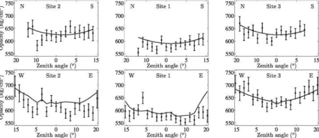
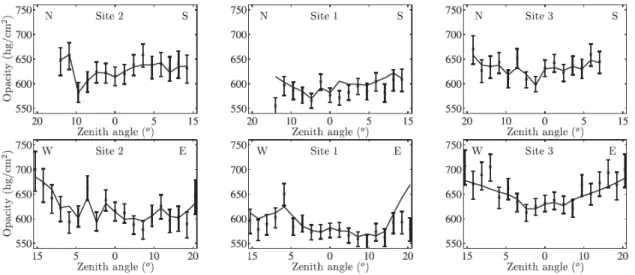
Figure 7. Comparison of the opacity estimated from the final model obtained with the 2-D inversion (solid lines) to the one deduced from the muon flux measurements (crosses).
The whole data set is used in the inversion but the inversion parameters contain only one cell in the N-S direction. The opacity data estimated from the final model compared to the measured ones are presented Fig. 7. Since the density variations are fixed to a constant value in the N-S direction, estimated opacity fluctuations in that direction is only due to thickness variations. For zenith angles
of view away from a zenith angle of 0° muon paths through the massif are indeed longer. In the E-W direction, estimated opacity values show relatively smooth variations from an angle of view to another. Due to the 2-D approximation, estimates from the inverse model only fit in average the measurements. Variations for a given telescope from an angle of view to another are not explained, however the inverse model resolves the opacity discrepancy observed in measurements from the three sites. The resulting density image shows a very low density zone in the Aalenian layer just above site 1 (Fig. 8). Three cells constitute the low density region, they present densities between 0.2 and 1.4 g cm-3 with a decreasing trend from W to E. The standard deviation is deduced from a Metropolis run
around the final solution obtained with the simulated annealing. Standard deviations of densities in the Aalenian layer above site 1 are the highest with a maximum value of 0.4 g cm-3 (Fig. 8). In the rest
of the domain densities are higher than 2.45 g cm-3 with a standard deviation around 0.15 g cm-3 or
lower, so the contrast of the low density region is significant.
Figure 8. Inversion result in 2-D. Top: density distribution of the final model, white lines indicate the fault locations as observed from galleries or surface. Bottom: standard deviation of the density values.
Such low densities can be interpreted by the presence of voids corresponding to karstic caves that could have developed on the stratigraphic interface above the Toarcian layer of very low permeability and along vertical fractures. In the upper layers density values are globally higher than 2.65 g cm-3
with a standard deviation around 0.15 g cm-3. A zone with lower density is visible in the lower Bajocian
with values around 2.3 g cm-3, other cells of the limestone medium present density values slightly
inferior to the global high density value. The presence of local variations in the limestone matrix porosity or local fractures could explain the density variations. The upper limestones layers are known to be heterogeneous as shown by electrical resistivity images (Gelis et al. 2010, 2015). However the
low density voxels in limestones do not form a pattern that could show density variations induced by fault structures observed on gallery walls.
6.2.
3-D INVERSION
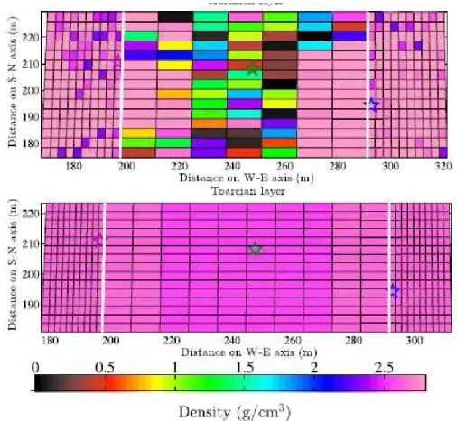
A 3-D inversion is applied to check the validity of a medium homogeneity along the N-S axis. Data are now better explained in the N-S and E-W directions compared to results with the 2-D approximation (Fig. 9). The resulting density image shows a very low density zone in the Aalenian layer just above site 1 (Fig. 8). The N-S corridor of low density is still observed in the Aalenian layer with values varying between 0 and 1.5 g cm-3 (Fig. 10). Here again the standard deviation presents higher values in that
low density region around 0.4 g cm-3 (Fig. 11) but densities in upper layers are also higher than 2.45 g
cm-3 with a standard deviation around 0.15g cm-3.
Figure 9. Comparison of the opacity estimated from the final model obtained with the 3-D inversion (solid lines) to the one deduced from the muon flux measurements (crosses).
Karstic voids explaining the low densities might present locally important height and width of 10-20 m. The lateral extension of the karstified zone is around 40 m and its position is located just above the fractured zone observed in the tunnel, interpreted as a strike-slip fault (Fig. 3). The presence of a such structure in the medium could influence water circulations along a preferential flow path following the structure in a N-S direction, and developing a karstic network gradually in the Aalenian limestones. Outcrops on the cliffs on the southern edge of the Tournemire massif show karstic features with openings coinciding with fault zones, supporting the hypothesis of a karstic network above galleries, but their extension and organisation remain unknown in the inner part of the Tournemire massif. Upward boreholes drilled from the tunnel testify the presence of an upper aquifer in the Aalenian. Those boreholes do not intercept karstic voids but karst networks are known to be very heterogeneous making the interception of conduits very unlikely. Karstic voids were not observed by previous geophysical explorations either. Their depth at more than 150 m from surface is actually too important to be observed from surface measurements. Their dimension is also relatively small compared to the resolution of geophysical methods which decreases with depth (Gelis et al. 2010). Geophysical methods suitable for karstic voids detection are discussed by (Chalikakis et al. 2011). Seismic or electrical resistivity methods are particularly adapted to characterize the ge-ometry of cavities but in the shallow region. The potential of seismic and electrical methods for detecting buried cavities was explored by (Grandjean & Leparoux 2004) and (Cardarelli et al. 2010) but
at depths lower than 20 m. Different experiments were performed in a karstic context to compare the capacity of both methods to distinguish air or water filled cavities until maximum depths of 50 m (Sheehan et al. 2005; Guerin et al. 2009; Valois et al. 2011). Moreover the presence of heterogeneities in the medium unease the detection of cavities (Grandjean & Leparoux 2004). Furthermore, the detection of buried cavities in the shallow subsurface requires an adapted configuration of the acquisition network optimized so the penetration depth and the image spatial resolution allow the observation of cavities on the resulting images. Rather than seeking the detection of 10 m height voids deeper than 150 m, surface geophysical experiments on the Tournemire massif were dedicated to the detection of faults and fractures. Such discontinuities were effectively well characterized in the near surface or below the clay layer (Cabrera 2005; Gelis et al. 2010, 2015). Recently an experiment of seismical imagery was performed in transmission between galleries where the telescope was installed and the surface (Vi Nhu Ba 2014). A region with low velocity is observed in the medium but its location in the Bajocian does not correlate with our very low density zone. Nonetheless the velocity image is obtained after a regularization process and the result strongly depends on the prior model that does not include voids. Moreover, geophones or sources located in the tunnel were placed on the ground and not on the galleries roof for facility reasons (Vi Nhu Ba 2014). The propagation of elastic waves might then be less sensitive to the presence of heterogeneities located just above the tunnel. Concerning the density contrasts in the upper layers, the 3-D images show a strong heterogeneity. However the interpretation of the density distribution in the Bajocian and Bathonian layers is not easy because of the irregularity of the density distribution. We note that the image does not show a structure that could indicate the presence of a fault zone in the Bajocian and Bathonian layers, in particular above site 1. Two reasons can explain that absence. First, the density contrast in the fault zone might be too low to be detectable. Second, the image resolution might be too coarse to allow the detection of a thin region presenting a density contrast with the surrounding medium. We explicitly choose to parametrize the inverse mesh with large voxels in order to limit the non-uniqueness of the inversion since the quantity of data collected—and so the quantity of information available—is small. Such a strategy allows insuring the stability of the inversion and the reliability of the resulting image. In order to improve the density image quality in a similar context two solutions might be considered to reduce the noise on the muon flux. The duration of the acquisitions could be extended to increase the statistics of the events. The acceptance of the sensor could also be reduced at the cost of a lower spatial resolution. However, refining the inversion mesh would require measuring data from at least two more acquisition sites in between sites 1 and 2 and sites 2 and 3 in order to supply complementary information on the medium density distribution. We emphasize the difficulty to distinguish the tectonic structures observed from galleries just above the tunnel with other geophysical methods. The perturbation of the medium induced by the observed tectonic structures might have been absorbed during the limestone layers sedimentation that was synchronous to the fault activity (Cabrera et al. 2001). Hence soundings above the galleries are seeking traces of perturbations that are susceptible to be more attenuated upward.
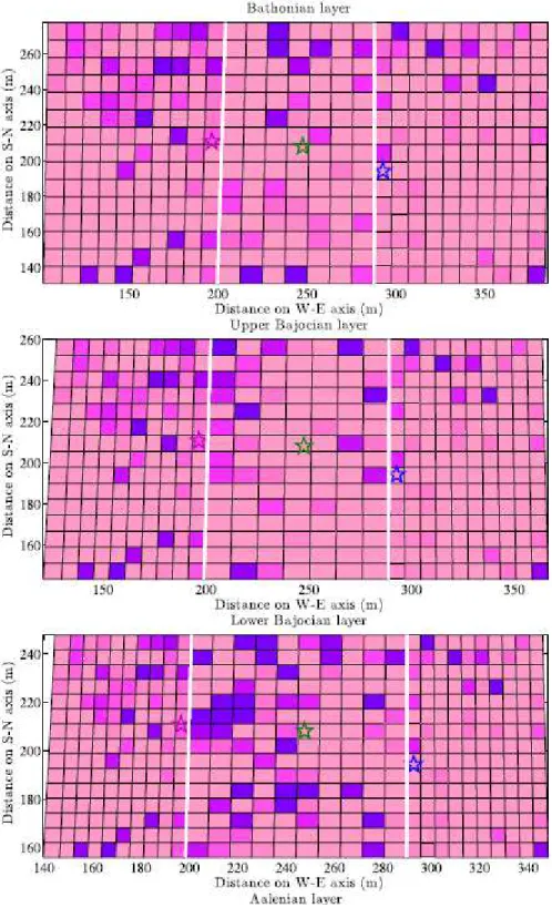
Figure 10. Density distribution at different elevation of the final model obtained with the 3-D inversion. Voxels outside the region delimited by white lines extend from the Toarcian top interface to surface (Fig. 6).
Figure 11. Standard deviation at different elevation of the final model obtained with the 3-D inversion. Voxels outside the region delimited by white lines extend from the Toarcian top interface to surface (Fig. 6).
7.
CONCLUSIONS
Muon flux measurements are directly sensitive to density variations in the medium, so average density values can be estimated along each direction of detection of a muon sensor. A network of telescopes detecting muons along trajectories that intersect in the medium is necessary to reconstruct the density distribution. The associated inverse problem non-uniqueness is strongly reduced compared to the one that aims at fitting gravimetric measurements sensitive to the density of the medium surrounding the gravimeter. In this study, muon flux measurements were performed from three sites in the underground galleries of the Tournemire experimental platform. The conversion of the measured muon flux into average density values evidenced the presence of a low density region located above one of the measurement sites. Then, data were analysed with a nonlinear 3-D inversion process giving insights on the resulting images reliability. A specific parametrization of the inverse problem allows the consideration of the acquisition network geometry and information provided by geological observations in order to reduce the inversion non-uniqueness. The resulting density image shows a N-S corridor of low density values in the Aalenian layer where the circulation of an aquifer is attested. The distinguished macroporous zone is interpreted by the presence of a karstic network. The presence of the clay layer of very low permeability below the Aalenian and the medium perturbation by faults observed on the gallery walls support this interpretation, as karsts formation and development are strongly influenced by pre-existing structures (Bakalowicz 2005). The karstified region presenting an important macroporosity extends laterally on a distance of about 40 m and might locally presents caves of decametric dimensions. The upward extension of the medium perturbation due to tectonic structures in upper layers is not evidenced from the density images. The heterogeneity of the upper limestones, attested by electrical resistivity measurements (Gelis et al. 2010, 2015), is also observed on the 3-D density images.
ACKNOWLEDGEMENTS
This work was financially supported by the IRSN through the experimental research project fund TOMUEX. We are very grateful to J.C. Sabroux for its enthusiastic support and the fruitful scientific discussions we had. We also thank Stephane Mazzotti for his advices on writing the manuscript. The comments and suggestions from Colin Farquharson and an anonymous reviewer have significantly improved the quality of the paper. The implementation of the experiment benefited from the great help of P. Desveaux, B. Combes and E. Martinez. Density estimates from the clay samples were performed by G. Alcalde and E. Barker. Muon flux measurements were performed with a sensor developed by the Diaphane collaboration and we appreciated greatly the participation of J.C. lanigro, S. Gardien, K. Jourde, D. Gibert and J. de Bremond d’Ars to the sensor preparation, its field installation and maintenance.
REFERENCES
Alvarez, L.W. et al., 1970. Search for hidden chambers in the pyramids, Science, 167, 832-839.
Ambrosino, F. et al., 2015. Joint measurement of the atmospheric muon flux through the Puy de Dôme volcano with plastic scintillators and Resistive Plate Chambers detectors, J. geophys. Res., 120, doi:10.1002/2015JB011969.
Bakalowicz, M., 2005. Karst groundwater: a challenge for new resources, Hydrogeol. J., 13(1), 148-160. Bhanot, G., 1988. The metropolis algorithm, Rep. Prog. Phys., 51(3), 429457.
Bretaudeau, F., Gelis, C., Leparoux, D., Brossier, R., Cabrera, J. & Cote, P., 2013. High-resolution quantitative seismic imaging of a strike-slip fault with small vertical offset in clay rocks from underground galleries: Experimental platform of Tournemire, France, Geophysics, 79(1), B1-B18.
Bryman, D., Bueno, J. & Jansen, J., 2015. Blind test of Muon geotomography for mineral exploration, in 24th International Geophysical Conference and Exhibition, 2015 February 15-18, Perth, Australia.
Cabrera, J., 2005. Evaluation de la methode sismique 3D haute résolution pour la detection de failles a deplacement subhorizontal. IRSN unpublished report DEI/SARG/2005-050.
Cabrera, J. et al., 2001. Projet Tournemire: synthese des résultats des programmes de recherche 1995/1999. IRSN report.
Calcagno, P., Chils, J.P., Courrioux, G. & Guillen, A., 2008. Geological modelling from field data and geological knowledge: part I. Modelling method coupling 3D potential-field interpolation and geological rules, Phys. Earth planet. Inter., 171(1), 147-157.
Carbone, D., Gibert, D., Marteau, J., Diament, M., Zuccarello, L. & Galichet, E., 2014. An experiment of muon radiography at Mt Etna (Italy), Geophys. J. Int, 196(2), 633-643.
Cardarelli, E., Cercato, M., Cerreto, A. & Di Filippo, G., 2010. Electrical resistivity and seismic refraction tomography to detect buried cavities, Geophys. Prospect., 58(4), 685-695.
Carloganu, C. et al., 2013. Towards a muon radiography of the Puy de Dôme, Geosci. Instrum. Methods Data Syst., 2, 55-60.
Chalikakis, K., Plagnes, V, Guerin, R., Valois, R. & Bosch, F.P., 2011. Contribution of geophysical methods to karst-system exploration: an overview, Hydrogeol. J., 19(6), 1169-1180.
Constantin, J., Peyaud, J.B., Vergely, P., Pagel, M. & Cabrera, J., 2004. Evolution of the structural fault permeability in argillaceous rocks in a polyphased tectonic context, Phys. Chem. Earth, 29(1), 25-41.
Cosenza, P., Ghorbani, A., Florsch, N. & Revil, A., 2007. Effects of drying on the low-frequency electrical properties of Tournemire argillites, Pure appl. Geophys., 164(10), 2043-2066.
Davis, K. & Oldenburg, D.W., 2012. Joint 3D of muon tomography and gravity data to recover density, in 22nd International Geophysical Conference and Exhibition, 2012 February 26-29, Brisbane, Australia.
Gaisser, T., 1990. Cosmic Rays and Particle Physics, Cambridge Univ. Press.
Gelis, C., Revil, A., Cushing, M.E., Jougnot, D., Lemeille, F., Cabrera, J., De Hoyos, A. & Rocher, M., 2010. Potential of electrical resistivity tomography to detect fault zones in limestone and argillaceous formations in the experimental platform of Tournemire, France, Pure appl. Geophys., 167(11), 1405-1418.
Geélis C. Noble, M., Cabrera J. Penz, S. & Chauris H. Cushing, M., 2015. Ability of high-resolution electrical resistivity tomography to detect fault and fracture zones: application to the Tourne- mire experimental platform, France, Pure appl. Geophys., 1-17, doi:10.1007/s00024-015-1110-1.
Groom, D.E., Mokhov, N.V. & Striganov, S.I., 2001. Muon stopping power and range tables 10 MeV-100 TeV, At. Data Nucl. Data Tables, 78(2), 183-356.
Guerin, R., Baltassat, J.M., Boucher, M., Chalikakis, K., Galibert, P.Y., Girard, J.F. & Plagnesn V. & Valois, R., 2009. Geophysical characterisation of karstic networks—application to the Ouysse system (Poumeyssen, France), C.R. Acad. Sci., 341(10), 810-817.
Guillen, A., Calcagno, P., Courrioux, G., Joly, A. & Ledru, P., 2008. Geological modelling from field data and geological knowledge: part II. Modelling validation using gravity and magnetic data inversion, Phys. Earth planet. Inter., 171(1), 158-169.
Grandjean, G. & Leparoux, D.2004. The potential of seismic methods for detecting cavities and buried objects: experimentation at a test site, J. Appl. Geophys., 56(2), 93-106.
Jardani, A., Revil, A., Santos, F., Fauchard, C. & Dupont, J.P., 2007. Detection of preferential infiltration pathways in sinkholes using joint inversion of self-potential and EM-34 conductivity data, Geophys. Prospect., 55(5), 749-760. Jourde, K., 2015. Un nouvel outil pour mieux comprendre les systemes volcaniques : la tomographie par muons, application a la Soufriere de Guadeloupe, PhD thesis, Univ. Paris 7, Paris, France.
Jourde, K., Gibert, D., Marteau, J., de Bremond d’Ars, J., Gardien, S., Girerd, C., Ianigro, J.C. & Carbone, D., 2013. Experimental detection of upward going cosmic particles and consequences for correction of density radiography of volcanoes, Geophys. Res. Lett., 40(24), 6334-6339.
Jourde, K., Gibert, D. & Marteau, J., 2015. Improvement of density models of geological structures by fusion of gravity data and cosmic muon radiographies, Geosci. Instrum. Methods Data Syst., 5, 83-116.
Kirkpatrick, S., Gelatt, C.D. & Vecchi, M.P., 1983. Optimization by simulated annealing, Science, 220(4598), 671-680.
Leroy, P., Revil, A., Altmann, S. & Tournassat, C., 2007. Modeling the composition of the pore water in clayrock geological formation (Callovo-Oxfordian, France), Geochim. Cosmochim. Acta, 71(5), 1087-1097.
Lesparre, N., Gibert, D., Marteau, J., Declais, Y., Carbone, D. & Galichet, E., 2010. Geophysical muon imaging: feasibility and limits, Geophys. J. Int., 183(3), 1348-1361.
Lesparre, N., Marteau, J., Declais, Y., Gibert, D., Carlus, B., Nicollin, F. & Kergosien, B., 2012a. Design and operationofa field telescope forcosmic raygeophysicaltomography, Geosci. Instrum. Methods Data Syst, 1, 3342.
Lesparre, N., Gibert, D. & Marteau, J., 2012b. Bayesian dual inversion of experimental telescope acceptance and integrated flux for geophysical muon tomography, Geophys. J. Int., 188, 490-497.
Lesparre, N., Gibert, D., Marteau, J., Komorowski, J.C., Nicollin, F. & Coutant, O., 2012c. Density Muon radiography ofLa Soufriere of Guadeloupe: first results and comparison with other tomography methods, Geophys. J. Int., 190(2), 1008-1019.
Lesparre, N., Boyle, A., Grychtol, B., Cabrera, J., Marteau, J. & Adler, A., 2016. Electrical resistivity imaging in transmission between surface and underground tunnel for fault characterization, J appl. Geophys., 128, 163-178.
Li, Y. & Oldenburg, D., 1998. 3-D inversion of gravity data, Geophysics, 63(1), 109-119.
Marteau, J., Gibert, D., Lesparre, N., Nicollin, F., Noli, P. & Giacoppo, F., 2012. Muons tomography applied to geosciences and volcanology, Nucl Instrum. Methods Phys. Res. A, 695, 23-28.
Marteau, J., de Bremond d’Ars, J., Gibert, D., Jourde, K., Gardien, S., Girerd, C. & Ianigro, J.C., 2014. Implementation of sub-nanosecond time-to-digital convertor in field-programmable gate array: applications
totime-of-flightanalysisinmuonradiography, Meas. Sci. Technol., 25(3), 035101,
doi:10.1088/0957-0233/25/3/035101.
Matray, J.M., Savoye, S. & Cabrera, J., 2007. Desaturation and structure relationships around drifts excavated in the well-compacted Tournemire’s argillite (Aveyron, France), Eng. Geol., 90(1), 1-16.
Metroplis, N., Rosenbluth, A W, Rosenbluth, M.N., Teller, A.H. & Teller, E., 1953. Equation of state calculations by fast computing machines, J. Chem. phys., 21(6), 1087-1092.
Nicollin, F., Gibert, D., Lesparre, N. & Nussbaum, C., 2010. Anisotropy of electrical conductivity of the excavation damaged zone in the Mont Terri Underground Rock Laboratory, Geophys. J. Int., 181(1), 303-320.
Nishiyama, R., Tanaka, Y., Okubo, S., Oshima, H., Tanaka, H.K.M. & Maekawa, T., 2014. Integrated processing of muon radiography and gravity anomaly data toward the realization of high-resolution 3-D density structural analysis of volcanoes: case study of Showa-Shinzan lava dome, Usu, Japan, J. geophys. Res., 119(1), 699-710.
Okay, G., Cosenza, P., Ghorbani, A., Camerlynck, C., Cabrera, J., Florsch, N. & Revil, A., 2013. Localization and characterization of cracks in clayrocks using frequency and time-domain induced polarization, Geophys. Prospect.,
61(1), 134-152.
Olive, K.A. et al., 2014. The review of particle physics, Chin. Phys. C, 38, 090001, Available at: http://pdg.lbl.gov/2014/ AtomicNuclearProperties/index.html.
Pessel, M. & Gibert, D., 2003. Multiscale electrical impedance tomography, J. geophys. Res., 108(B1), 2054, doi:10.1029/2001JB000233.
Portal, A. et al., 2013. Inner structure of the Puy de Dome volcano: crosscomparison of geophysical models (ERT, gravimetry, muon imaging), Geosci. Instrum. Methods Data Syst., 2, 47-54.
Sheehan, J.R., Doll, W.E., Watson, D.B. & Mandell, W.A., 2005. Application of seismic refraction tomography to karst cavities, in US Geological Survey Karst Interest Group Proceedings, Rapid City, South Dakota, 12-15.
Sugita, T. et al., 2014. Cosmic-ray muon radiography of UO2 fuel assembly, J. Nucl. Sci. Technol., 51(7-8), 1024-1031.
Tanaka, H.K.M., Nagamine, K., Nakamura, S.N. & Ishida, K., 2005. Radiographic measurements of the internal structure of Mt. West Iwate with near-horizontal cosmic-ray muons and future developments, Nucl. Instrum. Methods A, 555(1), 164-172.
Tanaka, H.K.M. et al., 2010. Three-dimensional computational axial tomography scan of a volcano with cosmic ray muon radiography, J. geophys. Res., 115(B12), doi:10.1029/2010JB007677.
Tang, A., Horton-Smith, G., Kudryavtsev, V.A. & Tonazzo, A., 2006. Muon simulations for Super-Kamiokande, KamLAND, and CHOOZ, Phys. Rev. D, 74, 053007, doi:10.1103/PhysRevD.74.053007.
Tarantola, A., 2005. Inverse Problem Theory and Methods for Model Parameter Estimation, SIAM, 342 pp. Valois, R., Camerlynck, C., Dhemaied, A., Guerin, R., Hovhannissian, G., Plagnes, N., Rejiba, F. & Robain, H., 2011. Assessment of doline geometry using geophysics on the Quercy plateau karst (South France), Earth Surf Process.
Landf., 36(9), 1183-1192.
Vi Nhu Ba, E., 2014. Detection des zones de failles par tomographie en transmission : Application a la Station Experimentale de Tournemire, PhD thesis, Ecole Nationale Superieure des Mines de Paris, 214 pp.
Yven, B., Sammartino, S., Geraud, Y., Homand, F. & Villieras, F., 2007. 2007. Mineralogy, texture and porosity of Callovo-Oxfordian argillites of the Meuse/Haute-Marne region (eastern Paris), Bull. Soc. Geol. Fr., 178, 73-90.