Towards Engineering a Web-Scale Multimedia Service: A Case Study Using Spark

HAL Id: hal-01416089

https://hal.inria.fr/hal-01416089

Submitted on 14 Dec 2016

HAL is a multi-disciplinary open access

archive for the deposit and dissemination of

sci-entific research documents, whether they are

pub-lished or not. The documents may come from

teaching and research institutions in France or

abroad, or from public or private research centers.

L’archive ouverte pluridisciplinaire HAL, est

destinée au dépôt et à la diffusion de documents

scientifiques de niveau recherche, publiés ou non,

émanant des établissements d’enseignement et de

recherche français ou étrangers, des laboratoires

publics ou privés.

Towards Engineering a Web-Scale Multimedia Service:

A Case Study Using Spark

Gylfi Guðmundsson, Laurent Amsaleg, Björn Thor Jónsson, Michael Franklin

To cite this version:

Gylfi Guðmundsson, Laurent Amsaleg, Björn Thor Jónsson, Michael Franklin. Towards Engineering a

Web-Scale Multimedia Service: A Case Study Using Spark. [Research Report] Inria Rennes Bretagne

Atlantique; Reykjavik University; UC Berkeley. 2016. �hal-01416089�

Towards Engineering a Web-Scale Multimedia Service:

A Case Study Using Spark

Gylfi Þór Guðmundsson

[email protected]

Laurent Amsaleg

[email protected]

Björn Þór Jónsson

[email protected]

Michael J. Franklin

[email protected]

ABSTRACT

Computing power has now become abundant with multi-core machines, grids and clouds, but it remains a challenge to harness the available power and move towards gracefully handling web-scale datasets. Several researchers have used automatically distributed computing frameworks, notably Hadoop and Spark, for processing multimedia material, but mostly using small collections on small clusters. In this pa-per, we describe the engineering process for a prototype near-web-scale multimedia service using the Spark frame-work running on the AWS cloud service. We present exper-imental results using up to 43 billion SIFT descriptors from the public YFCC 100M collection, making this the largest high-dimensional feature collection reported in the litera-ture. The design of the prototype and performance results demonstrate both the flexibility and scalability of the Spark framework for implementing multimedia services.

1.

INTRODUCTION

Computing power is now abundant with multi-core ma-chines, grids and clouds. Recently, many researchers have therefore investigated the use of automatically distributed computing frameworks (ADCFs), mainly Hadoop and Spark, to implement a variety of multimedia-related tasks. As these ADCFs do not provide the response time required to imple-ment interactive services for large multimedia collections, the focus of these works has been on background tasks, such as batch processing and indexing. These tasks focus on the throughput of the processing pipeline—how many items can be processed per second—rather than the response time. ∗_{This work was done while visiting the AMPLab at Berkeley} using an Inria fellowship.

.

1.1

Throughput-Oriented Services

Some examples of such throughput-oriented service arise on web-scale content sharing sites, where many background processes could be run, such as: a service that checks copy-right for detecting violations or monetizing content; a ser-vice to process and re-format content; and a serser-vice to au-tomatically classify newly uploaded content with e.g. face recognition or other classifiers for automated tagging. And there are yet more application domains, where large-scale batch-processing of multimedia tasks is important.

It is therefore of significant interest to the multimedia community to study the engineering process and require-ments for a throughput-oriented web-scale multimedia ser-vice. This paper presents a case study, where we imple-ment a large-scale copyright violation detection service us-ing Spark, and apply it to the largest available experimental feature collection.

1.2

Summary of Results

We show that the Spark pipelines required for indexing and batch processing are not overly complex, and can be easily extended for state of the art multimedia techniques. In terms of performance, processing scales well, both as col-lection size grows and as the number of processing units grows, and excellent throughput can be achieved. Finally, it is possible to implement batched index maintenance, but performance is not excellent and novel methods are required to improve maintenance performance.

We also report on our experiences of working with Spark, as well as working with a feature collection of 43 billion SIFT features, making it the largest experimental collec-tion of high-dimensional features reported in the literature. In short summary, any development at this scale remains very time-consuming. As an example, transforming the fea-ture collection from its original compressed text format to binary format took weeks, while storing the resulting com-pressed collection cost hundreds of dollars per month. It is clear, however, that having a well-developed ADCF, such as Spark, will certainly make such development easier for future generations of multimedia system engineers.

1.3

Overview of Paper

Sec-tion 2 discusses previous work using ADCFs to implement multimedia services and processes, and identifies six require-ments for such ADCFs. Section 3 then describes the design choices we made in this project, keeping in mind that our goal is not to develop new multimedia techniques, but to in-vestigate the engineering and performance requirements of web-scale services. Section 4 describes the prototypical al-gorithm used in our service and its implementation in Spark, as well as how the pipelines could be extended to implement other state of the art multimedia methods, and ends with a discussion of the engineering effort required for this study. Finally, Section 5 presents our performance results, before we conclude in Section 6.

2.

BACKGROUND

In recent years, the world has seen phenomenal growth in data creation and storage requirements. A very large pro-portion of that growth consists of multimedia files, such as images and videos. For example, Facebook claims to store more than 250 billion images, while Youtube users collec-tively upload more than three hundred hours of video every minute. As a result, there has been significant interest in the scalability of content-based multimedia retrieval [4, 13, 28, 12, 29].

In 2011, J´egou et al. proposed an indexing scheme based on the notion of product quantization and evaluated its per-formance by indexing 2 billion vectors [12]. Also in 2011, Lejsek et al. described a version of the NV-tree that in-dexes 2.5 billion local feature vectors [14]. In 2015, Babenko and Lempitsky used the inverted multi-index to index the BIGANN dataset, containing 1 billion features [3]. Finally, in 2015 Amsaleg reports results using the NV-tree to index a collection of 28.5 billion local features [1]. All these ap-proaches are centralized, however, and focus on the response time of the retrieval.

In 2007, Liu et al. reported the earliest distributed work indexing more than a billion high-dimensional feature vec-tors, but two thousand workstations were used to index the 1.5 billion vectors [15]. Sun et al. relies on the aggregation scheme proposed by [13], indexing 1.5 billion feature vec-tors from as many images, but using 10 servers [29]. The first example of implementing multimedia tasks on Hadoop is the work of Zhang et al. [38]. Since then multiple sim-ilar systems have been proposed, but mostly working with relatively small collections (e.g., see [7, 25, 35, 6, 34]). Im-ageTerrier [8] used the largest collection of these, indexing 10.9 million images using BoW features based on about 10 billion SIFT descriptors. Such systems have also seen some use in the medical image retrieval domain, again with rela-tively small collections [6, 34, 9]. The largest experiments on Hadoop indexed and searched around 100M images, or about 30 billion SIFT descriptors, using a cluster of 100+ machines [17].

Hadoop and Spark have also found use in other domains related to multimedia. Brandyn et al. used Hadoop to im-plement various computer vision tasks [33], experimenting with the k-means algorithm clustering about 200GB of data. More recently, Wang et al. proposed a library for Spark to improve performance of image retrieval [32]. While only k-means is described in detail, the library contains multiple algorithms for descriptor creation, image retrieval and result processing. Their experiments focus on small collections of less than 500 million descriptors. The KeyStoneML project

includes various machine learning algorithms implemented on top of Spark; one is a pipeline for object recognition using Fisher Vectors and SVM. In other recent projects, ADCFs were used for the training phase of deep learning processes, where massive collections feed the network to determine its parameters [21, 19].

2.1

Requirements for ADCFs

By studying the state-of-the-art literature and observing the needs of various multimedia services, we have gathered the following six common requirements that we believe an ADCF should meet in order to form a good basis for imple-menting web-scale multimedia services:

R1: Scalability: ability to scale out with additional com-puting resources as more and more data is handled. R2: Computational flexibility: ability to carefully

bal-ance system resources as needed.

R3: Capacity: ability to gracefully handle data that vastly exceeds main memory storage capacity.

R4: Updates: ability to gracefully update the data struc-tures for dynamic workloads.

R5: Flexible pipelines: ability to easily implement vari-ations of the indexing and/or retrieval process. R6: Simplicity: efficient use of implementer time through

simplicity of code.

In the remainder of this paper, we discuss how well the Hadoop and Spark ADCFs satisfy these requirements.

2.2

Map-Reduce and Hadoop

Map-Reduce is from Google [5] and exploits data inde-pendence through the Map and Reduce user-level functions. The input data is split into blocks stored on the participat-ing nodes usparticipat-ing a distributed file system such as HDFS [27]. The framework favors processing data locally, transparently handles the scheduling of tasks, and deals with communica-tions when nodes send/receive records to process.

Previous work, however, has shown that while Hadoop is good for solving a particular type of big data problems it fails at adequately solving the issues that multimedia systems raise [17]. For example, there are no facilities for updating the collection, the pipeline is very simple and rigid, and the code required to implement even elementary retrieval pro-cesses is complicated. Thus, Hadoop does not satisfy all of the six requirements listed above: Hadoop does scale out and can balance computations for large collections (require-ment R1), but it fails with all the other require(require-ments.

Let us consider these drawbacks in more detail. Hadoop forces systems to use a single input source—the HDFS data blocks. Many multimedia services use two sources of data, such as retrieval systems at indexing time, which need a codebook in addition to the data that must be indexed. Hadoop allows mappers to load distributed variables at launch time, so one such variable can store the codebook. But since mappers on the same physical node cannot share the main memory allocated for that variable, the codebook must be loaded again and again by each mapper, even when running on the same node. Hadoop thus only partially supports re-quirements R1 through R3.

.map

The .map() operator is a 1-to-1 transformation of each element into a new RDD of equal size. Example use cases: type conversions (int to long or text to number) or re-keying a key-value pair RDD.

.flatmap

The .flatmap() operator is a 1-to-any transfor-mation as each element invocation can return a list of new elements that are flattened into a new RDD. Example use case: splitting lines of text into words.

.groupByKey

The .groupBy() operator invokes a shuffle of the RDD to group the elements. The .group-ByKey() operator does the same for key-value pair RDDs, returning an RDD where each value is an iterator of the key’s elements.

.reduceByKey

The .reduce() operator reduces all elements of an RDD into a single instance. The .reduce-ByKey() operator is the key-value RDD equiv-alent, reducing all elements of the same key into a single value. Example use case: sum-ming numeric values.

.collectAsMap

The content of an RDD can be collected as an Array from the workers to the Master with the .collect () operator or as a hierarchical map structure with .collectAsMap().

.leftOuterJoin

Several join operators are available for com-bining two key-value pair RDDs into one. All invoke a shuffling of both RDDs into a new key-value pair RDD with access to the com-bined data via an iterator tuple.

.persist

The .persist (storage-level ) operator is used to tell Spark where to keep an RDD after instanti-ation. The storage level defaults to in-memory.

Table 1: Common RDD operators in Spark.

Hadoop fails with R4 (updates) because it cannot easily add new features to the existing data structures. Old and new vectors must be merged outside Hadoop, then stored within HDFS, and indexing is therefore done (almost) from scratch. This full re-indexing is pure waste as it is duplicated work for all but the new features.

The inflexible two-step Map-Reduce architecture is also causing troubles. Its is extremely difficult to run iterative or recursive processes such as a k -means which is often used to create codebooks. Workarounds require embedding Hadoop tasks inside high-level wrapping code repeatedly invoking Hadoop [22]. Having multiple sources or levels of codes leads to complications and poor performance. Hadoop therefore fails at statisfying requirements R5 and R6.

2.3

Spark

Central to Spark is the notion of a Resilient Distributed Dataset (RDD) [37, 36], a distributed data structure on disk or in memory. Spark facilitates transforming and manip-ulating RDDs in order to meet application needs and al-lows chaining operations in arbitrarily deep and complex pipelines. Spark defines many operators to manipulate the RDDs; the most common operators are listed in Table 1, which also introduces a graphical notation for the operators used in the remainder of this paper.

Spark typically uses HDFS as its file system. Data in an RDD is thus typically partitioned and spread out over the

computing cluster machines and Spark manipulates the data where it resides. Spark allows the programmer to choose to persist RDDs to various storage-levels (e.g., RAM or sec-ondary storage). Keeping RDDs in RAM preserves the per-formance of algorithms with iterative/recursive access pat-terns repeatedly scanning data.

Spark uses a Master-Worker workflow where the main code base is executed on the master and the distributed exe-cutions operating on an RDD flow out to the workers. Spark uses a lazy execution model where operations on RDDs are chained together until it becomes necessary to instantiate the data. Lazy execution facilitates optimizations.

A major goal of our study is to determine how well Spark satisfies the six requirements identified above; this is dis-cussed in Sections 4 and 5.

3.

DESIGN CHOICES

In this case study, we are primarily interested in under-standing the pros and cons of using Spark and cloud-based processing to implement (near) web-scale multimedia ser-vices. To that end, we decided to implement a multime-dia task for the study with a) a feature collection of tens of billions of features, and b) a workload representing both background processing and an on-line multimedia service.

3.1

Choice of Multimedia Tasks

The only application in the literature handling tens of billions of features is the DeCP algorithm, which is a proto-typical multimedia retrieval algorithm that has been applied to copy detection using a collection of 30 billion local fea-tures using the Hadoop ADCF [17]. This algorithm has a number of useful features for our study:

• The implementation and performance of DeCP has been studied extensively, including the impact of solid state disks, multi-core machines, and distributed pro-cessing (with Hadoop).

• It is a simple clustering and retrieval algorithm that is easily explained, understood, and implemented; yet is efficient and distributes well.

• The DeCP algorithm has both a pre-processing task (creating the clustered index) and a subsequent online task (batched image retrieval), and is thus representa-tive of many different types of multimedia services. • While the algorithm is simple, it can easily be extended

to work with state of the art methods, such as bags-of-features. In Section 4.3, we show how to implement such pipelines.

• The DeCP algorithm has been shown to give results of high quality for the copy detection case, even at a scale of 30 billion features.

As discussed in Section 2, the Hadoop implementation of DeCP highlighted some of the shortcomings of Hadoop for multimedia tasks. Since the aim of Spark was to address some of those shortcomings, it is also interesting to imple-ment DeCP on Spark to study whether the intended benefits of Spark materialize for this multimedia retrieval algorithm. We therefore focus on implementing DeCP on Spark.

3.2

Choice of Feature Collection

As our target is to study processing of a feature collec-tion containing tens of billions of features, the only realistic choice is to use SIFT features. While deep learning features have surpassed SIFT for some multimedia tasks, the SIFT features remain very competitive for partial copy detection. Most importantly, however, since a typical image yields hun-dreds of SIFT features, millions of images can yield billions of features. As we only have access to millions of images, this is the most important criterion for the feature collection.

Since the DeCP algorithm was developed in the context of the Quaero project, the feature collection from [17] is not publicly available. The largest experimental image col-lection available now is the recently developed YFCC100M collection; fortuitously the YLI collection of SIFT features computed from the YFCC100M collection was made avail-able just in time for our study. The YLI collection contains about 43 billion features, which require almost 7TB of stor-age, which is sufficient to really exercise the capabilities of the Spark system.

As it turned out, the SIFT features for YFCC100M were extracted using an implementation of SIFT that differs from the ones used when extracting local descriptors from ex-isting ground-truth such as Holidays [10], Copydays [11], Oxford5k [23], Paris6k [24] or other well established bench-marks. As a result, we can unfortunately not report quality metrics in this study. However, the DeCP algorithm has al-ready been shown to yield results of good quality, even at a comparable scale. Furthermore, various versions of SIFT exist and have been compared. They all prove to be quite equivalent and very stable in terms of recognition capabili-ties across implementations. We are therefore confident that the quality results obtained with DeCP and reported in [17] would not radically differ when using the YFCC collection as distractors, instead of the unavailable Quaero set of dis-tractors. And, most importantly, the target of our study is not the retrieval quality, but understanding the pros and cons of using Spark to implement multimedia related tasks.

3.3

Choice of Experimental Environment

We are interested in the use of cloud processing for mul-timedia tasks. As the workplace of the first author at the time had an agreement with Amazon that provided Amazon Web Services (AWS) credits, it was an obvious choice to use AWS for our experiments.

This choice has both benefits and drawbacks. The ben-efits include the fact that the YFCC100M collection, and the associated SIFT feature collection, were made available on AWS, reducing storage requirements. The drawbacks include difficulties obtaining reliable performance measure-ments. In particular, since we had to use a low-price resource allocation policy, experiments were frequently cut short due to pricing peaks.

3.4

Choice of (No) Baseline Comparisons

Aside from the previous work on DeCP using Hadoop, there are no existing studies at this scale to compare to. As our collection is larger and the computing hardware is rad-ically different, we can only discuss the differences between our results and those of [17].

3.5

Research Questions

We are primarily interested in understanding the pros and

cons of using Spark and cloud-based processing to implement (near) web-scale multimedia services. To that end, we are specifically interested in the following research questions:

1. What is the complexity of the Spark pipelines for typ-ical multimedia-related tasks?

2. How well does background processing scale as collec-tion size and resources grow?

3. How does batch size impact throughput of an online service?

In the next two sections we answer these questions for the particular case of DeCP running on Spark. It is our belief that since the application is quite representative for many multimedia-related tasks, as discussed above, our conclusion will generalize to many other multimedia tasks.

4.

PROTOTYPE IMPLEMENTATION

We start with a brief description of the DeCP algorithm before presenting its implementation on top of Spark. We then discuss using Spark to go beyond the prototypical al-gorithm and implement alternative state-of-the-art indexing approaches. Finally, we summarize the engineering effort of our project, and discuss how well Spark satisfies the require-ments R1 through R6.

4.1

The DeCP Algorithm

DeCP is quite representative of the core principles that are underpinning many unstructured quantization-based high-dimensional indexing algorithms and its extremely simple search procedure covers a large spectrum of existing ap-proaches. For example, we later show how DeCP can be modified to mimic not only the seminal VideoGoogle ap-proach [28], but also its descendants, with minimal changes to the Spark code.

DeCP uses a codebook learned over some data to guide the index construction. During the indexing phase, each im-age feature is assigned to the closest codeword(s), thereby forming clusters. Searching implements an approximate k -NN search process since only a single matching cluster (or a few) is scanned at search time. To improve scalability by lowering the cost of identifying the matching cluster(s), DeCP uses a multi-level hierarchy of codewords, as in many other approaches (e.g., [20]). When indexing very large fea-ture collections with DeCP (say, a few billion feafea-ture vec-tors) best practice calls for creating a few million clusters, each grouping about 15K features vectors (to utilize IO oper-ations well), along with a codebook hierarchy of 3 to 5 levels (to minimize CPU cost). As many other state of the art ap-proaches, DeCP may use soft assignment and multi-probing to increase the quality of results (see [24]). Finally, DeCP can easily process large batches of queries, searching up to a few million query vectors at the same time, maximizing throughput at the expense of response time.

DeCP has been shown to return approximate results of good quality at very large scale. It has been used to exe-cute large batches of queries against extremely large image feature collections (up to 30 billion SIFT descriptors). Its design principles, its architecture, some implementation de-tails and performance results have been published in various venues [17, 26, 18].

Input RDD = N features

Codebook .map

RDD (codewordID , feature) .groupByKey

RDD (codewordID , feature iterator ) .map

RDD (codewordID , feature array) Output RDD = C clusters

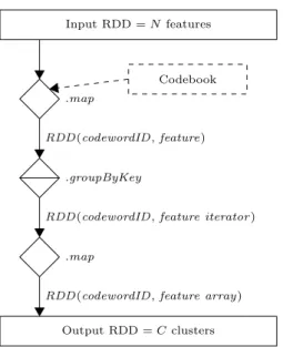
Figure 1: Spark pipeline for indexing (quantization).

4.2

DeCP on Spark

We now describe the implementation of DeCP on top of Spark: the pipeline for creating the codebook and assigning the feature vectors to the codewords at index construction time; the pipeline which implements the k-NN search pro-cess; and the pipeline for index maintenance.

4.2.1

Index Construction

The feature collection must be stored on HDFS before the index construction can start. The codebook for DeCP is created by randomly sampling the feature vectors using the .take() command. The sampled vectors are organized top-down into a multi-level tree, which is then pushed to persistent storage by writing it as a serialized object file.

The pipeline for quantizing, i.e., assigning feature vectors to codewords, is a rather straightforward chain of RDD op-erators, shown in Figure 1. The codebook is first broadcast to all workers, as shown using the dashed arrow in the fig-ure. The RDD with the feature vector collection is then chained to a .map() operator which i) reads the input data and ii) traverses the codebook to determine the codeword that is the closest to each input feature vector. This first .map() operator produces a new RDD made of key-value pairs, where each pair is composed of the codewordID as the key and the current feature vector as the value, thus representing the assignment of each feature vector to a clus-ter. That RDD is then chained to a .groupByKey() operator which groups the pairs according to the key, the codewordID in this case, which essentially shuffles the data across the network in order to prepare for the final cluster formation. As a technical detail, the .groupByKey() operator produces a new key-value RDD where the value is an iterator, so a final .map() operator is needed to convert the iterators into arrays such that the RDD can be serialized and stored to disk. At that point, the features vector have been assigned to clusters which are in turn distributed using HDFS.

When this pipeline is executed, the underlying distribu-tion of the feature vector data on HDFS is inherited by the initial RDD instantiation. Subsequent RDDs, resulting from shuffling or other Spark operators, may be distributed

differ-ently. Recall that RDDs are instantiated only when needed and are transient, unless persisting operators are used ex-plicitly, so the whole pipeline is executed at the same time.

4.2.2

Batch Searching

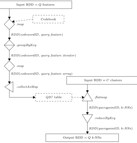
The DeCP query pipeline starts by creating an RDD from all the query feature vectors in the query batch. The code-book of the index is then loaded to identify the codeword that is most relevant for each query vector. Once this is done, the queries can be grouped according to their code-wordID , which shows which query vector requires data from which cluster. This is, again, the same pipeline as the one used in the initial steps of the index creation, albeit with one difference. As many other state-of-the-art multimedia retrieval systems, DeCP may use multi-probing at search time [24]. With multi-probing, multiple codewords are in-volved per query and multiple clusters must therefore be scanned, possibly on different machines, each resulting in intermediate k-NN lists that must be merged and consoli-dated to eventually form the final k-NN of the query.

Figure 2 shows the batch search pipeline. The start of the pipeline creates an RDD that associates codewordID to queryID , resulting in an RDD which contains the query-to-codeword table (Q2C , top half of Figure 2). Note that the RDD might contain several entries for each queryID due to multi-probing. Entries in the Q2C table are grouped using .groupByKey() according to the values of codewordID . This table is collected and broadcast to all nodes (dashed arrow). The bottom half of Figure 2 shows the remaining part of the pipeline. A .flatmap() operator reads the indexed RDD, as well as the broadcast Q2C table, and determines the k-NN of each query point for each codeword that is con-cerned by this query batch. This is the main operation of the pipeline, where neighbors are matched with query features. This creates another RDD of pairs with queryID as the key and the k-NN as the value. Here again, multiple pairs with the same queryID key may exist due to multi-probing, so the next step in the pipeline is to merge and consolidate the multiple intermediate k-NN lists that exist for each query. This is done using a .reduceByKey () operator that produces a unique k-NN result list per query vector.

Note that the Hadoop version of DeCP did not support multi-probing as there was no efficient way to handle the two reduction steps that are required. To implement multi-probing in Hadoop, it is required to push to HDFS all the in-termediate k-NN lists, and then initiate a second full MapRe-duce job to load these lists, perform the merge and consol-idate the lists. In addition to the costly launch overhead of Hadoop, the performance would suffer seriously due to writing and then reading data on secondary storage. In contrast, this process is easy and efficient with Spark as: transformations of RDDs can be chained; RDDs remain in main memory; and the whole pipeline is a single job.

4.2.3

Index Maintenance

Index maintenance refers to adding a set of feature vectors to a previously indexed collection1 and proceeds as follows. First, the new feature vectors are assigned to codewords in much the same manner as during index construction: the codebook created for the previously indexed collection must be loaded; the new collection of features must be

trans-1_{Deletion can be implemented similarly, with the addition}

Input RDD = Q features

Codebook .map

RDD (codewordID , query feature) .groupByKey

RDD (codewordID , query feature iterator ) .map

RDD (codewordID , query feature array)

.collectAsMap Q2C table Input RDD = C clusters .flatmap RDD (querypointID, k-NNs) .reduceByKey RDD (querypointID, k-NNs) Output RDD = Q k-NNs

Figure 2: Spark pipeline for batch k-NN search.

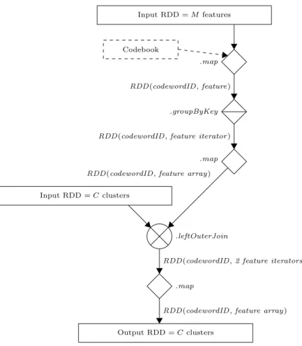
formed into an RDD; and the codeword for each new feature must be determined and the new features grouped according to their corresponding codewordID . This pipeline, shown in the top half of Figure 3, results in an RDD where the newly added feature vectors are grouped by clusters, ready to be merged into the existing index.

Two options are possible for the merge, depending on whether the RDD holding the new feature vectors fits in the RAM of the least equipped machine or not. If that RDD is small enough, then it is best to merge the new vectors to the existing index with a .map() or .flatmap() operation. This will create a new RDD with the appended data, which must then be pushed to local storage. This option incurs some moderate network traffic, as the new vectors must be broadcast to all the participating machines.

Otherwise, if the RDD of new features is too large, then it is best to join-merge that RDD with the RDD holding the existing index. In this case, the pipeline must include a .leftOuterJoin() operator that will shuffle both RDDs and group the records with the same key on the same worker. The pipeline must then include a .map() operator to com-bine the records of the two RDDs that can subsequently be pushed to storage. This option causes much more network traffic as the full data collection and the new vectors may all be shuffled. This latter pipeline is shown in Figure 3.

We have also tried other options, utilizing the flexibility of Spark to assemble operators in complex pipelines. We tried a pipeline where the new vectors are not added to the

existing collection but are instead used to create a second index that is also probed at query time. Of course, the nearest neighbors of query points determined for each index must be merged to form the final result. It is also possible to design a pipeline where a sequential search against the most recent features is performed while the index over the existing collection is probed. This pipeline can speed-up the index maintenance as it batches the updates of new features, but it slows down search as merging intermediate results is again needed. Therefore, there is an interesting trade-off where the application programmer can optimize the behav-ior of its multimedia retrieval system over Spark for index maintenance or for retrieval.

4.3

Beyond DeCP: Advanced Pipelines

Multimedia retrieval systems in real life typically include features that are not part of the DeCP approach described above. Furthermore, state-of-the-art systems may use tech-niques that slightly differ from the ones used in DeCP, which has been designed as a prototypical retrieval system. In par-ticular, a fully functional multimedia retrieval system must extract feature vectors from the media file and we first show how external Computer Vision libraries can be linked to Spark. We then describe how secondary similarity measures can be added to DeCP in order to re-rank candidate images. This allows, e.g., the implementation of a voting process or weak geometry verifications when dealing with local feature vectors. Finally, we show how DeCP can be extended to

im-Input RDD = M features

Codebook

.map RDD (codewordID , feature)

.groupByKey RDD (codewordID , feature iterator )

.map RDD (codewordID , feature array) Input RDD = C clusters

.leftOuterJoin

RDD (codewordID , 2 feature iterators) .map

RDD (codewordID , feature array) Output RDD = C clusters

Figure 3: Spark pipeline for index maintenance.

itate the high-dimensional indexing strategies derived from the seminal Bag-Of-Words (BoW) paradigm [28].

4.3.1

Extracting Features from Media

So far we assumed that feature vectors were already ex-tracted from the images and ready for indexing and query-ing. It is possible, however, to extend the pipelines sketched above to include a feature extraction step. First, the mul-timedia material must now be stored in HDFS. The next step is to run the feature extraction code, in a distributed manner, saving the resulting high-dimensional vectors into a new RDD using .map() and .persist (). This step must be added to the pipelines of Figures 1 and 2, but the pipelines are otherwise identical to what was described before.

Connecting a Java library (e.g., BoofCV) to Spark is triv-ial, but it is more complicated to connect a C/C++ library. Spark can invoke legacy code with the .pipe() operator but that only passes text via std-in and -out, which is not suit-able for large volumes of high-dimensional features. Another alternative is relying on JNI to wrap the legacy library, al-lowing invocations from .map() or .flatmap() operators. Tra-ditional computer vision libraries can thus be utilized (such as OpenCV or VLFeat), allowing the extraction of state-of-the-art feature vectors such as MFCC (for audio), SIFT, SURF, or the more sophisticated VLAD features [2]. This is, for example, done in the ML-Lib vision pipeline, where a JNI wrapper allows using VLFeat to extract dense SIFT features [31].

4.3.2

Secondary Similarity Measures

Various motivations have driven researchers to use sec-ondary similarity measures in multimedia retrieval systems, including removing false positives, trying to defeat the curse of dimensionality, and compensating for the asymmetry of NN-based similarity. Typically, the traditional primary k-NN similarity creates a list of candidates, which is then pro-cessed using a secondary similarity measure to re-rank the candidates; the top elements of the re-ranked list are then returned to the user. It is possible to equip DeCP on Spark with such secondary similarity measures and in the following we give two examples that are representative of techniques found in the literature.

The first example is a voting-based secondary similarity measure, for example needed when using local features such as SIFT [16]. With local features, each image, including the query, is described using many feature vectors. The similarity is established first by identifying the k-NN of each query local feature and then by making each identified local feature “vote” for the image it belongs to. Once all the query local features have been used to probe the index, the images with the most votes are returned as the most similar.

The vote aggregation process in Spark requires adding op-erators to the search pipeline in order to transform the RDD that contains the consolidated k-NN lists. This RDD groups the lists according to their queryID . It is necessary to read this RDD and reshuffle its data according to the imageID using a .reduceByKey () followed by a .map() that will count

the number of votes each image receives from the collection. Note that all the experiments described in the next section use this vote aggregation secondary similarity measure.

The second example re-ranks the candidate images ac-cording to an estimate of the degree of geometric consis-tency of angles and scales between the query and the can-didate images [10]. Pushing consistent images up in the ranking, and inconsistent images down, is easy as geometry and scale information is integrated into the feature vectors. Unlike most systems, a costly re-extraction of the vector in-formation from the candidate images is not needed as we can simply include the original feature vectors in the search pipelines RDD with very minimal code changes. The ac-tual post-process of re-ranking can then be appended to the pipeline using the necessary RDD transformations: for ex-ample, .flatmap() to compare randomly chosen sets of fea-ture vectors in the result to the corresponding sets of original query features (already in memory in the Q2C table), and .reduceByKey () to gather the geometric results per image and output the final re-ranked results. The Hamming em-bedding approach discussed in [10] can also be implemented in a similar fashion.

4.3.3

Imitating BoW

The Bag-Of-Words (BoW) approach was originally pro-posed by Sivic and Zisserman [28]. Many extensions and improvements have subsequently been proposed, making the BoW approach a seminal contribution to the field of high-dimensional indexing. BoW basically applies to images tex-tual information retrieval techniques where the words of the document collections are recorded in a vector model with a cosine-based metric and a tf-idf -based secondary similarity measure. With images, the local image features are turned into “visual words” using a visual codebook and features are clustered with their closest codeword. Each local query fea-ture votes for all the images assigned with the closest code-word(s), so scanning the clusters to search for the closest vectors is in fact not needed.

This impacts the pipeline as some Spark operators can be removed and the code simplified. Early in the pipeline, it is not necessary to create an RDD where the features from the collection to index are kept; instead it is only necessary to keep track of which featureID gets assigned to which code-wordID . The resulting RDD is much smaller (as the com-ponents of the features are not needed) so it can potentially remain in (the distributed) main memory, thus enhancing performance. Stripping the featureID from an existing in-dexed dataset can be done using a .map() operator. The subsequent .flatmap() is also simplified, as the code for scan-ning the selected cluster(s) is not needed anymore.

4.4

Discussion

In this section, we have described the engineering pro-cess for a prototypical (near) web-scale multimedia service implemented on top of Spark. We have described how we were able to take advantage of the flexibility built into Spark, both with respect to the advanced resource management and the flexible pipeline construction.

As an example of the former, Spark is able to use main memory very effectively, meaning that on Spark the scal-ability of DeCP is only bound by the amount of RAM per machine and not by the amount of RAM per core, as was the case in Hadoop. We believe that the requirements of

scal-ability, computational flexibility and capacity, R1 through R3, can all be satisfied quite well by Spark. We have also described how to implement a form of dynamic index man-agement that goes some way towards satisfying the update requirement R4. In the next section we show experimental results which further support these claims.

As an example of the latter, we have shown how Spark’s flexibility and deep pipelines provide the tools necessary to implement a full-feature system seamlessly, and we have also described how some common post-processing steps, such as re-ranking, can be added with minimal overhead and code changes. None of this was considered remotely feasible with Hadoop [17]. This discussion thus shows that the require-ments for flexibility and simplicity of pipelines, R5 and R6, are satisfied very well. The support for the last two require-ments is perhaps best articulated by the following three ob-servations: a) we are able to build a full-feature system with relatively easily explained pipelines; b) we can often propose more than one way to solve the same task; and c) we have proposed numerous extensions to implement more complex pipelines with very modest code changes.

We also learned that working with collections at this scale is most akin to “running in syrup”. Compressing the feature collection from text format to binary format, for example, took weeks, while storing the resulting compressed collection cost hundreds of dollars per month. During our work we hit several bugs in Spark, which slowed our progress. Fortu-nately, we observed that projects in other application areas had often concurrently identified the same issues, so most of these were resolved relatively soon. However, detecting, isolating and uncovering each such bug typically took weeks, making this engineering project a massive undertaking.

However, given the rate of improvements between Spark versions, as well as the results reported below, we conclude that Spark has very strong potential for implementing vari-ous families of large-scale multimedia services.

5.

EXPERIMENTS AND RESULTS

5.1

Experimental Setup

We have run our experiments on the Amazon Web Ser-vices (AWS), using C3.8xl nodes. Each node has 60GB of RAM, 640GB of SSD storage, an E5-2680 CPU at 2.8GHz with 32 virtual cores (vCores). Intel hyper-threading tech-nology is used for half of these vCores; this is known to perform worse than a true core. We have in all cases used 51 of these C3.8xl nodes to create the Spark cluster. The cluster is thus composed of 1 master and 50 slaves, for a to-tal of 1600 vCore workers. This configuration allows using 2.8 TB of RAM and 30 TB of HDFS SSD storage in total.

Our feature collection is the recent publicly available YLI corpus, which consists of 42,949,150,170 SIFT visual features derived from 96,560,779 Creative-Commons-licensed Flickr images [30]. We converted the features to a binary format stored as an RDD in our S3 bucket; in total the collection requires about 7TB of disk space. To facilitate running ex-periments at various scales, we partitioned the 43 billion feature collection into five roughly equals parts. Each of the five parts, referred to as a, b, c, d and e respectively, contains approximately 8.5 billion SIFT descriptors and oc-cupies about 1.4TB of disk space. We believe that we are reporting the first experiments using the full SIFT collection of the YLI corpus, and hence the largest feature collection

Indexing Relative Scaling vCores Time (s) Observed / Optimal

400 5,931 — / — 800 3,510 0.59 / 0.50 1600 3,287 0.55 / 0.25

Table 2: Experiment #1: Scaling out index creation.

ever used in the literature.

To index the collection (and the various sub-collections) we created a 5-level codebook that defines 20 million code-words. We have intentionally used a large codeword hierar-chy which can accommodate much more than the YLI col-lection. With 43 billion features, only about 2,100 features are assigned to each codeword on average (or about 425 for each of the five parts a through e), while it is good prac-tice to fit between 15 and 50 thousand features per code-word [18]. The codebook hierarchy used here could thus gracefully, with absolutely no change, scale to indexing 500 billion to a few trillion descriptors with only a linear increase in the time required for quantization. Note that the over-head for traversing this hierarchy and managing so many codewords negatively impacts the index creation and search times that we report, as a 4-level codebook defining 2 to 4 million codewords would have been more appropriate for indexing 43 billion features; the overhead is of course even worse when indexing smaller sub-collections.

Note that aside from basic Spark parameter tuning, we have done little in terms of optimization. We run the Spark framework “out-of-the-box” and none of the authors are ex-perts in either Java or Scala. Furthermore, we deploy our cluster in AWS where accurate monitoring of the environ-ment is limited due to virtualization and concurrency.

5.2

Experiment #1: Scaling Out Resources

The first experiment observes the ability of Spark to scale out; how the execution time decreases in proportion to the increase in hardware resources. We focus on the index con-struction (the most CPU intensive pipeline) of a relatively small sub-collection (a). To measure the ability to scale out, we set a Spark configuration parameter (spark.cores.max) to limit the number of vCores used to 400, 800 or all 1600 vCores. Recall that the first 800 vCores are true hardware cores while the last 800 vCores are hyper-threading cores.

The performance of the index creation pipeline against these three AWS configurations is summarized in Table 2. It’s second line is when hyper-threading cores are not used. Doubling the number of vCores in use nearly divides in half the time it takes to run the index creation. The added over-head of using 800 true cores instead of 400 is 18% above the optimal, see the Observed/Optimal column.

Above 800, the added cores are hyper-threading vCores. While the number of vCores is doubled, the quantization time is only reduced by about 7% (third line of Table 2). This is caused by the poor performance of hyper-threading cores as indicated by Intel’s guide-lines and observed in work on Hadoop [17, 26].

5.3

Experiment #2: Scaling Up Collection

This second experiment is intended to observe the ability of the system to scale up; how the execution time evolves when indexing larger and larger collection with the same

Indexing Relative Collection Descriptors Time (s) Scaling

a 8.5B 3,287 —

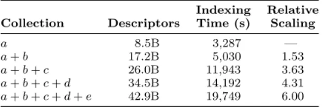
a + b 17.2B 5,030 1.53 a + b + c 26.0B 11,943 3.63 a + b + c + d 34.5B 14,192 4.31 a + b + c + d + e 42.9B 19,749 6.00

Table 3: Experiment #2: Scaling up index creation.

hardware. For this experiment, we use the full 1600 vCores of the 50 C3.8xl AWS worker nodes. We measure the wall clock time for running the index creation pipeline against five feature collections of increasing size, ranging from a to the full collection of 43 billion descriptors.

The wall clock time for the indexing (quantization) is re-ported in Table 3. It takes 3,287 seconds to complete the index creation pipeline when indexing the a sub-collection. Indexing the full 43 billion features takes 19,749 seconds, or about six times longer. As the last column of Table 3 indi-cates, the system scales up quite well with larger collections. The indexing time for the largest collection is about 5.5 hours, which can be decomposed into about 2.5 hours for as-signing each feature vector from the collection to its appro-priate codeword and about 3 hours to achieve the shuffling process grouping the descriptors into clusters. Note that despite using as many as 1600 vCores, only 50 machines were used and they had to shuffle about 7TB of data, which severely stresses the communication links.

5.4

Experiment #3: Full Scale Batch Search

This experiment examines the performance of searching the full scale collection with batches of query images. We have built batches of queries by sampling the collection, re-sulting in up to 80,000 images in a single batch, each having about 400 query features, for a total of up to 32 million query features in a single batch.

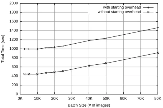
We use the 51 C3.8xl nodes. The codebook is the 5-level hierarchy organizing 20 million codewords. Each experiment is an end-to-end batch-search job, where the wall clock run-ning time of the entire job is measured. Note that the wall clock time includes the time required to load the codebook at job launch time, about 550 seconds, which is something a live system would only do once.

In this experiment, multi-probing is not used and the number of neighbors collected for each query point is set to k = 20. In this discussion we focus on the time to process the batch and the corresponding throughput.2

The time it takes to entirely process batches of queries are given by Figure 4. It takes about 1,000 seconds to process the smallest batch, which contains 2,500 images, while it takes close to 1,500 seconds to process the largest batch of 80,000 images. Multiplying the size of the batch by 32 thus increases the response time only by a factor of 1.5: larger batch requires relatively little more disk activity to read clusters, while utilizing CPUs much better.

Figures 5 and 6 show the time per image and throughput, respectively, both with and without the time required to

2_{As discussed in Section 3, we do not report quality}

indica-tors here, as a) no ground truth is available for the YLI fea-ture collection and b) the DeCP algorithm has been shown to return good results at a similar scale.

0 200 400 600 800 1000 1200 1400 1600 1800 2000 0K 10K 20K 30K 40K 50K 60K 70K 80K

Total Time (sec)

Batch Size (# of images)

with starting overhead without starting overhead

Figure 4: Experiment #3: Total running time.

0.00 0.05 0.10 0.15 0.20 0.25 0.30 0.35 0.40 0.45 0.50 0K 10K 20K 30K 40K 50K 60K 70K 80K

Time Per Image (sec)

Batch Size (# of images)

with starting overhead without starting overhead

Figure 5: Experiment #3: Search time per image.

0 10 20 30 40 50 60 70 80 90 100 0K 10K 20K 30K 40K 50K 60K 70K 80K

Throughput (images / sec)

Batch Size (# of images)

with starting overhead without starting overhead

Figure 6: Experiment #3: Batch search throughput.

load the codebook. As the figures show, the time required per image initially drops very fast as the batch size is in-creased, with a corresponding increase in throughput; the time required to process one query image from the batch drops from 0.39 seconds with the smaller image batch to 0.018 seconds when processing the largest batch. This sug-gests that with small batches most of the CPUs sit idle,

waiting for data to arrive. With larger batches, in contrast, the CPUs are more effectively used and the throughput of the system improves.

5.5

Experiment #4: Index Maintenance

This last experiment assesses the possibility to implement index maintenance instead of index re-creation. This is done by inserting a large collection of new features into an existing index and comparing the resulting performance to the per-formance obtained when re-indexing from scratch the aug-mented feature collection.

For this experiment, we use the a and b sub-collections, which contain 8.5B and 8.7B of SIFT features, respectively. We assume that we have sub-collection a already indexed and wish to add the sub-collection b. Note that the scale of the sub-collection calls for using the .leftOuterJoin() option, presented in Figure 3.

Our measurements showed that adding the data to the existing index took 3,855 seconds, while re-indexing took 5,030 seconds; it is thus more efficient to add data to an existing index than to re-create a larger index from scratch. Of course, the total time to index a and then merge b is higher than a single round of indexing, but once a is already indexed, the index maintenance pipeline is more efficient.

We believe, however, that Spark could be improved in this aspect as it does not have a specific method to join a small RDD to a much larger RDD. An efficient method of shuffling only the smaller RDD, followed by a local join to the larger RDD, could further improve index maintenance performance at large scale.

5.6

Discussion

One of the primary limitation of implementing even a ba-sic multimedia service in Hadoop [17] was that the scalability was bound by amount of RAM per core. As the collection size grows, larger data structures are typically needed for managing the collection (the cluster index, in the case of DeCP), which in turn require more RAM memory. This is not an issue with Spark, and in our experiments we even used a significantly larger index than needed to emphasize this difference.

Also, in contrast to the Hadoop implementation reported in [17], we implemented a full-featured system using Spark. This was not originally planned, as it was not until we started working with Spark that we realized how the various features of the framework made it easy for us to accommo-date the more complex pipelines. This is a clear testament to the simplicity and flexibility of the Spark framework.

Our experimental results reinforce our conclusion that Spark supports large-scale throughput-oriented multimedia services very well. We have investigated the performance of index construction and batch search, and shown that Spark scales both out and up. Using a grid of a hundred machines, DeCP on Hadoop needed more than half a second per im-age; in these experiments, however, a large batch results in an average time per image of less than 20 milliseconds! This is despite the fact the we are running experiments on heavily under-sized clusters, due to the over-sized index.

6.

CONCLUSIONS

In this paper, we have argued the advantages of using automatically distributed computing frameworks (ADCFs) to implement throughput-oriented multimedia services, in

order to cope with today’s very large and ever growing mul-timedia collections. We have identified six requirements that such ADCFs should satisfy, in order to effectively support multimedia services: Scalability; Computational flexibility; Capacity; Updates; Flexible pipelines; and Simplicity.

Much of the focus to date has naturally been on the pop-ular Hadoop framework with some promising results. How-ever, the limited flexibility of the two-step pipeline and lack of advanced features have been shown to impose restrictions on what can be reasonably and/or feasibly achieved [17].

To the best of our knowledge, we have engineered the first (near) web-scale multimedia service running on Spark: a full-featured off-line copy detection system (with multi-probing, search-expansion and post-process re-ranking). We have described in detail the Spark pipelines for index cre-ation, batch search, and index maintenance, and also dis-cussed how to implement many advanced CBIR approaches and extensions using Spark.

We have then measured the performance of the prototype by conducting some of the largest experiments reported to date, using 43 billion SIFT descriptors from the YFCC 100M collection. These experiments have have shown that Spark satisfies all six requirements identified for a high-throughput web-scale multimedia service. We therefore argue that de-signers of scalable multimedia services should strongly con-sider using Spark (or subsequent frameworks with similar capabilities) as the basis for their systems.

Acknowledgements

This work was made possible in part thanks to support from the Inria@SiliconValley program.

7.

REFERENCES

[1] L. Amsaleg. A database perspective on large scale high-dimensional indexing. Habilitation `a diriger des recherches, Universit´e de Rennes 1, 2014.

[2] R. Arandjelovic and A. Zisserman. All about VLAD. In Proc. CVPR, 2013.

[3] A. Babenko and V. S. Lempitsky. The inverted multi-index. TPAMI, 37(6), 2015.

[4] E. Y. Chang. Foundations of Large-Scale Multimedia Information Management and Retrieval: Mathematics of Perception. Springer, 2011.

[5] J. Dean and S. Ghemawat. Mapreduce: simplified data processing on large clusters. CACM, 51(1), 2008. [6] R. K. Grace, R. Manimegalai, and S. S. Kumar.

Medical image retrieval system in grid using Hadoop framework. In Proc. ICCSCI, 2014.

[7] C. Gu and Y. Gao. A content-based image retrieval system based on Hadoop and Lucene. In Proc. ICCGC, 2012.

[8] J. S. Hare, S. Samangooei, D. P. Dupplaw, and P. H. Lewis. ImageTerrier: An extensible platform for scalable high-performance image retrieval. In Proc. ICMR, 2012.

[9] S. Jai-Andaloussi, A. Elabdouli, A. Chaffai,

N. Madrane, and A. Sekkaki. Medical content based image retrieval by using the hadoop framework. In Proc. ICT, 2013.

[10] H. J´egou, M. Douze, and C. Schmid. Hamming embedding and weak geometric consistency for large

scale image search. In Proc. ECCV, 2008.

[11] H. J´egou, M. Douze, and C. Schmid. The Copydays image dataset. http:

//lear.inrialpes.fr/people/jegou/data.php\#copydays, 2008.

[12] H. J´egou, M. Douze, and C. Schmid. Product quantization for nearest neighbor search. TPAMI, 33(1), 2011.

[13] H. J´egou, F. Perronnin, M. Douze, J. S´anchez, P. P´erez, and C. Schmid. Aggregating local image descriptors into compact codes. TPAMI, 34(9), 2012. [14] H. Lejsek, B. T. J´onsson, and L. Amsaleg. NV-Tree:

Nearest neighbours at the billion scale. In Proc. ICMR, 2011.

[15] T. Liu, C. Rosenberg, and H. Rowley. Clustering billions of images with large scale nearest neighbor search. In Proc. WACV, 2007.

[16] D. G. Lowe. Distinctive image features from scale-invariant keypoints. IJCV, 60(2), 2004. [17] D. Moise, D. Shestakov, G. T. Gudmundsson, and

L. Amsaleg. Indexing and searching 100M images with Map-Reduce. In Proc. ICMR, 2013.

[18] D. Moise, D. Shestakov, G. T. Gudmundsson, and L. Amsaleg. Terabyte-scale image similarity search : experience and best practice. In Proc. Big Data, 2013. [19] P. Moritz, R. Nishihara, I. Stoica, and M. I. Jordan.

Sparknet: Training deep networks in spark. CoRR, abs/1511.06051, 2015.

[20] D. Nist´er and H. Stew´enius. Scalable recognition with a vocabulary tree. In Proc. CVPR, 2006.

[21] B. C. Ooi, K.-L. Tan, S. Wang, W. Wang, Q. Cai, G. Chen, J. Gao, Z. Luo, A. K. Tung, Y. Wang, Z. Xie, M. Zhang, and K. Zheng. Singa: A distributed deep learning platform. In Proc. ACM MM, 2015. [22] S. Owen, R. Anil, T. Dunning, and E. Friedman.

Mahout in Action. Manning Publications Co., 2011. [23] J. Philbin, O. Chum, M. Isard, J. Sivic, and

A. Zisserman. Object retrieval with large vocabularies and fast spatial matching. In Proc. CVPR, 2007. [24] J. Philbin, O. Chum, M. Isard, J. Sivic, and

A. Zisserman. Lost in quantization: Improving particular object retrieval in large scale image databases. In Proc. CVPR, 2008.

[25] W. Premchaiswadi, A. Tungkatsathan, S. Intarasema, and N. Premchaiswadi. Improving performance of content-based image retrieval schemes using Hadoop MapReduce. In Proc. HPCS, 2013.

[26] D. Shestakov, D. Moise, G. T. Gudmundsson, and L. Amsaleg. Scalable high-dimensional indexing with Hadoop. In Proc. CBMI, 2013.

[27] K. Shvachko, H. Kuang, S. Radia, and R. Chansler. The Hadoop distributed file system. In Proc. SMSST, 2010.

[28] J. Sivic and A. Zisserman. Video google: A text retrieval approach to object matching in videos. In Proc. ECCV, 2003.

[29] X. Sun, C. Wang, C. Xu, and L. Zhang. Indexing billions of images for sketch-based retrieval. In Proc. ACM MM, 2013.

[30] B. Thomee, D. A. Shamma, G. Friedland, B. Elizalde, K. Ni, D. Poland, D. Borth, and L.-J. Li. The new

data and new challenges in multimedia research. arXiv preprint arXiv:1503.01817, 2015.

[31] A. Vedaldi and B. Fulkerson. Vlfeat: An open and portable library of computer vision algorithms. In Proceedings of the 18th ACM international conference on Multimedia, pages 1469–1472. ACM, 2010. [32] H. Wang, B. Xiao, L. Wang, and J. Wu. Accelerating

large-scale image retrieval on heterogeneous architectures with Spark. In Proc. ACM MM, 2015. [33] B. White, T. Yeh, J. Lin, and L. S. Davis. Web-scale

computer vision using MapReduce for multimedia data mining. In Proc. MDM, 2010.

[34] Q.-A. Yao, H. Zheng, Z.-Y. Xu, Q. Wu, Z.-W. Li, and L. Yun. Massive medical images retrieval system based on Hadoop. JMM, 9(2), 2014.

[35] D. Yin and D. Liu. Content-based image retrieval based on Hadoop. Mathematical Problems in Engineering, 2013.

[36] M. Zaharia, M. Chowdhury, T. Das, A. Dave, J. Ma, M. McCauley, M. J. Franklin, S. Shenker, and I. Stoica. Resilient distributed datasets: A fault-tolerant abstraction for in-memory cluster computing. In Proc. NSDI, 2012.

[37] M. Zaharia, M. Chowdhury, M. J. Franklin, S. Shenker, and I. Stoica. Spark: cluster computing with working sets. In Proc. USENIX CHTCC, 2010. [38] J. Zhang, X. Liu, J. Luo, and B. Lang. DISR:

Distributed image retrieval system based on MapReduce. In Proc. PCA, 2010.