Convergence and conditioning issues with X-FEM in fracture mechanics

HAL Id: hal-02136900

https://hal.archives-ouvertes.fr/hal-02136900

HAL is a multi-disciplinary open access archive for the deposit and dissemination of sci-entific research documents, whether they are pub-lished or not. The documents may come from teaching and research institutions in France or abroad, or from public or private research centers.

L’archive ouverte pluridisciplinaire HAL, est destinée au dépôt et à la diffusion de documents scientifiques de niveau recherche, publiés ou non, émanant des établissements d’enseignement et de recherche français ou étrangers, des laboratoires publics ou privés.

Convergence and conditioning issues with X-FEM in

fracture mechanics

Éric Béchet, Hans Minnebo, Nicolas Moës, Bertrand Burgardt

To cite this version:

Éric Béchet, Hans Minnebo, Nicolas Moës, Bertrand Burgardt. Convergence and conditioning issues with X-FEM in fracture mechanics. WCCM VI in conjunction with APCOM’04, Sep 2004, Pékin, China. �hal-02136900�

Convergence and conditioning issues with X-FEM in fracture

mechanics

Eric Béchet1*_{, Hans Minnebo}1_{, Nicolas Moës}1 _{and Bertrand Burgardt}2

1 _{Institut de Recherche en Génie Civil et Mécanique}

Ecole Centrale de Nantes / Université de Nantes / UMR CNRS 6183 B.P. 92101, 1 Rue de la Noé, 44321 Nantes Cedex 3, France

2 _{SNECMA Moteurs, Rond Point René Ravaud – Réau, 77550 Moissy-Cramayel, France}

e-mail: [eric.bechet | hans.minnebo | nicolas.moes]@ec-nantes.fr, bertrand.burgardt@snecma.fr

Abstract Numerical crack propagation schemes were augmented in an elegant manner by the X-FEM

method applied to fracture mechanics. The use of special tip enrichment functions, as well as a discontinuous function along the sides of the crack allows one to do a complete crack analysis virtually without modifying the underlying mesh, which is of an evident industrial interest.

The conventional approach for crack tip enrichment (described in [2,3]) is that only a specific layer of elements are enriched around the crack tip. We show that this “topological” approach does not yield an increase of the order of the asymptotic convergence rate when compared to unenriched finite elements, as when the crack is part of the mesh. It rather modifies the proportionality factor of the asymptotic convergence rate. In this study, we propose another enrichment scheme which yields a convergence rate that appears to be close to that of regular finite elements used when the solution field does not show singularities.

The enriched basis in X-FEM degrades the rigidity and mass matrices condition numbers (the mass matrix typically appears in case of time dependent problems such as wave propagation in cracked bodies). To recover the condition number of non enriched matrices, we introduce a preconditioning strategy which acts block-wise on the set of enriched degrees of freedom associated to each node. This strategy uses a local (nodal) Cholesky based decomposition.

Another issue is brought by the integration scheme used to build the matrices. The nature of the asymptotic functions are such that any Gauss-Legendre based integration scheme will only poorly converge with respect of the order of the quadrature. We propose a modified integration scheme to handle that issue.

We apply the new technique developed to the estimation of stress intensity factors along the crack front of 3D cracks and use these SIFs for crack propagation using a Paris type fatigue law.

Key words: X-FEM, convergence rate, J-integral, preconditionner, crack propagation INTRODUCTION

Typical finite element analysis for crack propagation involved three major steps. The fists step consists in the construction of a mesh that is able to describe the crack geometry, as standard finite elements for mechanical problems are continuous. This is often cumbersome, because the geometry of the crack is independent of the CAD model. Moreover, when the crack evolves, the mesh should evolve in parallel, and keep its conformity with the crack geometry. The second step involves the computation of stress intensity factors. These are used to predict the path followed by the crack if a fatigue behavior is to be expected; or, in the case of a static load applied to the structure, to quantify the maximum load it can withstand before the crack becomes unstable. The computation of stress intensity factors must be carefully done using domain integrals, and cannot be inferred from local stresses or displacements obtained at the crack tip. This lead to non local SIFs evaluations in 3D, as the domain integrals must be

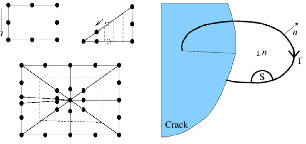
chosen as to avoid numerical inaccuracies at the crack tip. To further lower those inaccuracies and reduce the size of the domain integrals, special crack tip elements can be used. Among those, Barsoum [4] elements are a good choice if one wants to keep the standard finite elements approach. Barsoum elements rely on standard quadratic elements, on which some control points are moved to the quarter of the edges, in addition to the collapse of one of its faces (see Figure 1-a). There is few, if no, modifications of the finite element codes dealing with Barsoum elements. Nevertheless, Barsoum elements still lead to inaccuracies in the field at the crack tip impairing any attempt to determine SIFs with local, near tip, fields. The third and last step in crack path prediction involves the update of the crack front. As the crack is part of the mesh, this involve the update of the mesh, as well as the data structures associated to the crack geometry.

Fig. 1 – a) Barsoum elements around a crack tip in 2D, b) Contour integrals path.

The X-FEM method can handle most of these issues by means of the partition of unity [5,6]. The asymptotic near tip displacement field is included in the finite element basis, as well as a discontinuity eliminating the need of re-meshing. However, we will show in this study that the enrichment scheme commonly used in this approach lead to the same order of convergence than regular finite elements methods.

DOMAIN INTEGRALS

The evolution of the crack depends on crack tip parameters, namely stress intensity factors. These are computed using well known domain integrals that are easier to implement in finite element software than their theoretical contour integral counterpart. The transformation is done using Green's theorem. We recall briefly the expression of the density of energy release (3D case) from the Eshelby tensor for a

plane crack.   x3 lies on the edge of S  x3 , which is a planar material sheet of infinitesimal

thickness. Here, nj is the normal to the surface. On the edge; this is the exterior normal, it is parallel to

the plane S  x3 . vm is the virtual velocity of the crack at the considered location. The contour is

displayed on Fig. 1-b. P_mj=1  2 klklmj−ijui , m (1) j x3=

∮

∬

The global energy release rate on a segment of the crack front is the integral of the equation (2):

J=

∫



j dx_{3 (3)}

J=−

∭

∬

In this expression, is a weight function vanishing on the domain boundary. The resulting integral (4) is

in fact the weighted mean value of J over the domain V. If there are no forces acting on crack sides, the second part of the integral vanishes.

We use the same idea to compute interaction integrals [3] :

I_a₌₋

∭

∭

∬

The new eshelby-like tensor is defined as the following (see [7]), because of the main symmetry of the

elasticity tensor C_ijkl=C_klij:

P_mja _= klkl a_ mj−ij a_u i , m−ijui , m a ₍₇₎

, wherea,aand ua_{are the auxiliary fields for which everyK}

i a

is known. Using three distinct sets of

auxiliary fields Aa=

{

}

ia), one can eventually determine the values of

the stress intensity factors for the actual displacement field with the relation:

Ga =2 1− 2 E K1 K1 a K2 K2 a 1  K3 K3 a ₍₈₎ in which Ga= I a

∫

THE X-FEM METHOD

Enrichment The X-FEM method, based on the local PUM [2,3], uses elementary displacement fields

obtained from an infinite cracked body. There are 4 basic enrichment functions needed to span the Westergaard solution at the crack tip [8]:

F_ir ,=

{









}

In these functions, r and are polar coordinates respective to the crack front. Only elements immediately

around the crack tip are usually enriched with these functions (in the sequel, this will not be necessarily the case). Along the sides of the crack, the enrichment is chosen to be the Heaviside discontinuous function so that the resulting displacement field contains a discontinuity at the location of the crack:

H n=

{

−1  if n0

}

In this function, n is the signed distance computed normally to the crack sides. In the remaining of the domain, there is no enrichment so the conventional finite element basis is the only one existing. The resulting displacement field is :

uh=

∑

i∈R Nii

∑

∑

F_jij

∑

i∈HNiH i (12)

the domain), the set of nodes which need to be enriched for the tip functions, and the set of nodes for the Heaviside enrichment. The set of nodes H is determined to avoid an ill posed problem, as in [2].

i, ij, iare the coefficients of the displacement field, those are to be determined by solving the linear

system obtained after assembly.

Integration The integration in standard finite element codes is done with a Gauss quadrature. The

integration is generally exact because the terms are polynomials. In X-FEM, the same gauss quadrature is used but as enrichment functions are not polynomials, the integrations are not exact. This issue will be discussed in the sequel.

NEW ENRICHMENT PROCEDURES

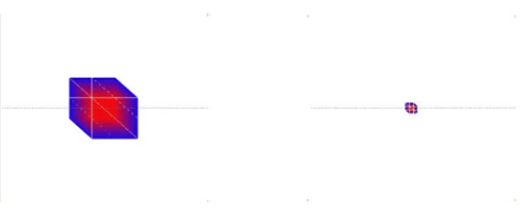
As said previously, the enrichment in X-FEM procedures (and inherently also procedures made with the Barsoum element) is such that only one layer of elements bears the complete enrichment basis (i.e. develop a partition of unity behaviour). In [9] this has been shown under certain circumstances to impair the accuracy of computations because a subsequent layer of elements are only partially enriched. This enrichment is referred later in the discussion as “topological”. The characteristic of this “topological” behaviour is that the the size of the enriched area is proportional to h. In opposite, we propose a “geometrical” enrichment, that bears the characteristic of a constant enriched area within a prescribed geometry. In fact, in [6], an implicit reference to additional layers of elements in the enriched area is briefly made. In the following figures, a comparison showing enriched areas for both methods within two levels of refinement is displayed. The criteria used to determine which nodes are enriched is such

that if one node lies within a circle of radius re, then it is enriched.

Fig. 2 Topological enrichment for h=1/10 (left) and h=1/50 (right)

Fig. 3 Geometrical enrichment for h=1/10 (left) and h=1/50 (right)

CONVERGENCE RESULTS

In this section we shall describe current results obtained using (a) a regular finite element procedure without enrichment, (b) results obtained by the X-FEM method with topological enrichment and (c) results obtained by a geometrical enrichment. The domain considered here is a 2-d unity patch under tension. The tension is such that it corresponds to an infinite cracked body loaded with a uniform

exact displacement field. As one can see on the mesh, the crack location is not along elements sides. The domain is a 1x1 square. In the case of a geometrical enrichment, it is made over a circular patch with

re=0.05 . In the case of a topological enrichment, it is made on the elements immediately around the

crack tip (1 layer).

Fig. 4 Mesh of the computational domain and exact displacement field under prescribed tension. The color range shows the magnitude of the displacement u.

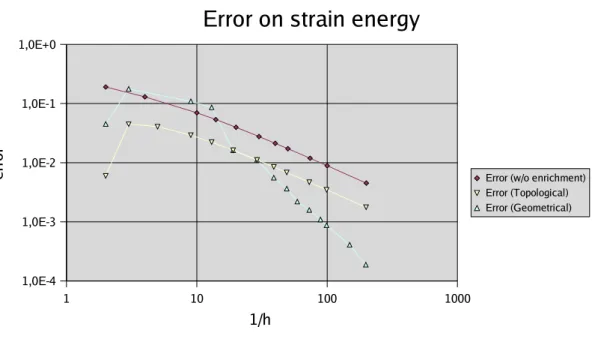
Error on strain energy The convergence results in relation with the element size h shows an

improvement as one choose to enrich in a geometrical way.

1 10 100 1000 1,0E-4 1,0E-3 1,0E-2 1,0E-1 1,0E+0

Error on strain energy

Error (w/o enrichment) Error (Topological) Error (Geometrical) 1/h er ro r

Fig. 5 Error on the strain energy versus element density (log-log scale)

In linear finite elements, when the solution displacement field is smooth, the theoretical rate of convergence of the strain energy is 2. This means that, if one reduce the size by a factor two, the error on the energy is divided by 4. When a crack is present in the domain, the theoretical rate of convergence decrease to 1. This appears on Fig. 5, which shows actual convergence results for unenriched as well as enriched displacement fields. When one choose to enrich the displacement field around the crack tip in a topological way, Fig. 5 also shows there is a constant shift toward lower errors when compared to unenriched finite elements. This means that this enrichement procedure does not improve the convergence rate as one could expect by the addition of exact displacement modes in the enriched field. When one chooses to enrich in a geometrical way, the usual rate of convergence for linear finite element is kept. This is shown again in Fig. 5. The convergence rate observed toward the right of the diagram is between 1.8 and 2.1 (this is not a smooth curve because the shape of the enriched domain changes as h decreases). In this calculation, the exact strain energy was computed on the exact displacement field

(known) with a gauss quadrature, on a highly refined mesh. We have made 3-dimensional computations as well, displaying nearly identical results (not showed here for the sake of conciseness).

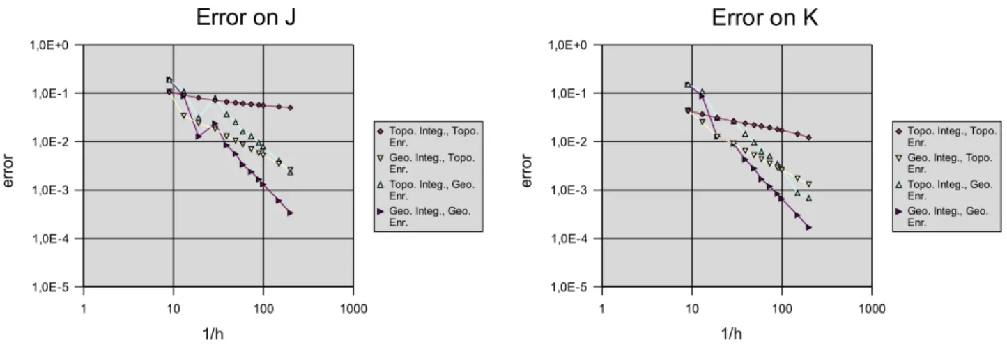
Error on J and K integrals The same study is made for the J and K integrals. However, there is one

more parameter, namely the size of the integration domain. We have defined two strategies : a domain whose size decreases with h , and a domain whose size is constant. This is very similar to the enriched area definition, so we shall call them later on with the same qualifiers : topological if the domain size is proportional to h and geometrical if it is constant. Thus, there are 4 cases to study. The problem studied here is the same as the one used for the strain energy error and, by construction, the exact solution for this problem is such that K=1 and J=1. The integration domain is a circular patch. Its radius is defined

as : ri = 0.15 if it is geometrical, and ri = 1.5h if it is topological (if h=1/10, both domains are the same).

In addition, it should be noted that J and K have here a local meaning.

The convergence results for J and K are shown on following figures. It is remarkable that there is a very slow convergence for a topological enrichment and a topological integration domain (first curve). In fact, this is the reason why one always recommend to increase the integration domain's size until convergence. There is a drawback to this : in the case of 3d calculations, the values obtained for J or K are not local (these are a mean value along the crack front). The second curve; which displays the convergence for a topological enrichment and a geometrical integration domain shows a convergence rate around 1.0, which is quite good.

In the case of a geometrical enrichment, results are much better. Even in the case of a topological

integration domain, there is convergence (the rate is in this case between 1.0 and 1.5, see 3rd _{curve for}

both J and K). This means that we are able to extract local information from the displacement field, and this even at the crack tip, which is an interesting feature. When both the enrichment and the integration domain are geometrical, the convergence rate is increased to around 2.0 for both J and K and provides the best approximations.

1 10 100 1000 1,0E-5 1,0E-4 1,0E-3 1,0E-2 1,0E-1 1,0E+0 Error on J

Topo. Integ., Topo. Enr.

Geo. Integ., Topo. Enr. Topo. Integ., Geo. Enr. Geo. Integ., Geo. Enr. 1/h er ror 1 10 100 1000 1,0E-5 1,0E-4 1,0E-3 1,0E-2 1,0E-1 1,0E+0 Error on K

Topo. Integ., Topo. Enr.

Geo. Integ., Topo. Enr. Topo. Integ., Geo. Enr. Geo. Integ., Geo. Enr.

1/h

er

ror

Fig. 6 Error on J and K versus element density (log-log scale)

PRECONDITIONNER

Description The above mentioned geometrical enrichment procedure produces ill-conditioned mass and

rigidity matrices since many degrees of freedom (dof) are enriched. The use of iterative solvers, even with “out of the box” built in preconditioners (incomplete LU among others) is difficult, especially in 3D when the number of degrees of freedom is high, as in a real industrial parts. We propose a specialized preconditioner for enriched finite elements. This preconditioner is not a substitute for general purpose preconditioners found in iterative solvers, its aim is to take advantage of the knowledge of the enrichment to produce linear systems that are easier to solve with out of the box preconditioners and solvers. The idea behind this specific preconditioning scheme is to orthogonalize the finite element basis generated for each regular degree of freedom. Let us consider the structure of the linear system Ku=f:

〚

a b ⋯

b c ⋯

⋱

〛

u=f (13)

In the case displayed here, there is only one enrichment at a time, for the sake of clarity. Thus; in addition to each regular dof, there is one enriched dof . This gives the size (2) of the sub-matrix showing terms a, b and c. We want those terms to be orthogonal, in order to solve the modified linear system :

〚

1 0 ⋯

0 1 ⋯

⋱

〛

u'=f' (14)

To obtain this result, we do a Cholesky decomposition (equation 15) of the sub-matrix, and uses this decomposition to pre- and post- multiply the adequate terms in the relation. The matrix G is completed with diagonal 1's to match the size of the original system. Of course the implementation is not exactly as described for evident performance issues, but it is mathematically equivalent.

〚

b c

〛

T

(15) The resulting system is then:

G K GT_u'

=Gf with u=GT_{u' (16)}

Results The following results were obtained on the same 2D patch used to test the new enrichment

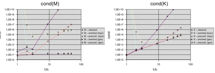
procedure. As a comparison, it should be mentioned that for linear finite elements without enrichment, the condition number of mass matrices tends to a constant whereas that of rigidity matrices is in order 1/h². With enrichment, and especially with geometrical enrichment; the condition number degrades very much as 1/h increases. 1 10 100 1,0E+0 1,0E+1 1,0E+2 1,0E+3 1,0E+4 1,0E+5 1,0E+6 1,0E+7 1,0E+8 1,0E+9 1,0E+10 cond(M) M – classical M – enriched (topo) M – precond. (topo) M – enriched (geo) M – precond. (geo) 1/h co nd 1 10 100 1,0E+0 1,0E+1 1,0E+2 1,0E+3 1,0E+4 1,0E+5 1,0E+6 1,0E+7 1,0E+8 1,0E+9 1,0E+10 cond(K) K – classical K – enriched (topo) K – precond. (topo) K – enriched (geo) K – precond. (geo) 1/h co nd

Fig. 8 Condition number of the mass and rigidity matrices versus element density (log-log scale)

In the case of the mass matrix M, the condition number is greatly reduced for both topological and geometrical enrichments. It is however still increasing with the mesh density in the case of a geometrical enrichement. For the rigidiy matrix K, the results are globally the same. In the case of a topological enrichment, one can see that the condition number for non preconditioned matrices is very close to the curve corresponding to regular finite elements. However, we observed that preconditioning allows one to solve big systems that were otherwise very difficult to solve using iterative solvers. When the enrichment was geometrical, even for moderately sized problems, standard iterative methods failed if we did not use that ad-hoc preconditioner.

INTEGRATION

The use of X-FEM, with enrichment functions, requires the ability to integrate singular functions. The

four crack tip functions are of the following type : F(r,θ)=



functions. The singularity occurs in the integrand of related terms, in the stiffness matrix. Those terms are the product of the gradient of two interpolation functions, possibly “enriched”. By substitution, we can easily find that the functions appearing in the integrand are a combination of

1/r , 1/













only the radial parts create difficulties for the integration. In the sequel, we focus on the integration of

gr , on a triangle where g is harmonic in  and singular in r.

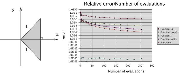
Up to now, triangular sub-elements are created, in order to integrate continuous functions. The singular point therefore lies on a vertex. As shown on the following example, the convergence achieved with a standard Gauss integration is very slow. The need for a better quadrature is clear.

0 50 100 150 200 250 300 1,0E-16 1,0E-15 1,0E-14 1,0E-13 1,0E-12 1,0E-11 1,0E-10 1,0E-9 1,0E-8 1,0E-7 1,0E-6 1,0E-5 1,0E-4 1,0E-3 1,0E-2 1,0E-1 1,0E+0

Relative error/Number of evaluations

Function 1/r Function 1/sqrt(r) Function 1 Function sqrt(r) Function r Number of evaluations er ro r

Fig. 9 Integration domain and convergence of a standard Gauss integration scheme

Another option available to integrate crack singularities is the use of the so-called “quarter-point” Barsoum element described earlier in the text [4]. The drawback of this method is that the mesh needs to be conforming to the problem. In 3D, this quadrature is valid only on edges of the elements.

Description of the singular mapping - The purpose is to integrate, in a fast way and within a prescribed

accuracy, the function gr , on a triangular patch. For this, we will map the real triangular element on

a reference quadrangular element. This way we transform singular functions into regular ones. The mapping is shown in Fig. 10, with Node 0 (singular one) corresponding to the reference edge “u=-1”.

On the reference element, “u” represents the radial coordinate, and “v” represents the orthoradial one. These coordinates are obtained after several coordinate changes starting from a polar transformation

r ,.

Details of the transformation We need to integrate the expression :

I=

∬





Here, g is a singular radial function.

We introduce the polar coordinates : xr ,=r cos  , y r ,=r sin  . In the following expression, r0

is the orthogonal distance of the opposite side to the singular node; it also gives the reference angle for  . We have then:

I =

∬

cos] ,  ∈ [1;2] (18)

We then use the following mapping in order to fit u in the interval [-1;1] and have polynomial terms

with respect to



∬

2 cosg  x r u , , , y r u , ,r u ,du d  with u ∈ [−1 ;1] ,  ∈ [1 ;2] (20)

In this expression, a term in cos −1 appears, which can be singular. We introduce then another

coordinate change “t” so that dt=cos −1_{d as proposed in [10]. It brings :}

t=1  2 ln





In a final step, to fit v in the interval [-1;1] , we set t=t1t2

2  t₂−t1 2 v . Then, =sin−1 tanh





∬

4 1ut2−t1g x r u ,v,v , y r u ,v ,vr u ,vdudv (23)

with u ,v ∈ [−1;1]2 _.

As a result, we have a polynomial part in “u”, and a smooth part in “v”. Both are easily integrated without too many sampling points.

Results As one can see on the next figure, the convergence has been highly improved for the five

functions on which the integrand is based. The results have been performed using the same number of Gauss points for each axis (u and v). The “singular mapping” is shown to be a good method to integrate singular functions. We studied mainly the radial influence, since the angular functions are smooth, and thus, easily integrated. However, if the triangle is narrow, the angular part will be well approximated with very few points, whereas if it is almost flat, it will have greater variations, so, more integration points will be required. We plan to investigate on this issue. The case of a singularity lying slightly out of an element has also still to be investigated, as the present method only applies to singularities located precisely at one vertex of the triangle. As for 3D integration, we propose to cut 3D elements orthogonally to the crack front and integrate each of the slices with the same quadrature.

� � ��� � � ��� � � ��� ������! ������ ������� ������� ������� ������� ������� �����" �����# �����$ �����! ����� ������ ������ ������ ������ ���� � %�����&��������'(�)����*��&��(������ +(��������������(��� +(����������,������ ���(��� +(������������(��� +(��������,������ ���(��� +(������������(��� +(���������������(��� +(����������,������ ����(��� +(�������������(��� +(��������,������ ����(��� +(�������������(��� '(�)����*��&��(������ �� �� � .���� ��$����������;$����� ������ ����������������$����������$;���@����� ���3������A� �!����*!"*�%� �"� �$�"((*�$1���$�@%$��($ A�1$#$*�($1��$%$�������%"�:�(%�("!"��������>E5���$������"*��%"�:�!$�2$�%&�� (*"�$ � "�1 � ��$ � �����"* � �%"�: � 9%��� � *�$ � �� � ��$ � 2�11*$ � �9 � " � =������L? � %$!�*"% � 2$ � � =1�2$� ��� � "%$ -5��-5���5�?5������$ $�%$ �*� ����$�$�%���2$����":$ �(*"�$��������"��&*��1$%��9�%"1�� ��5-� �((�%�$1�/&���$ �%"�:�9%���5���$�/���1"%&����1����� �"%$�-?����9�%2��$� ���������$��(($%�"�1�*��$%� �%9"�$��"�1��? ���9�%2� �$"%� �� � "**� �� �1$ 5� ��� $D�$��*&� � ��$� �%"�: � 9%���� 2� �� 9�**�� � "� :��:$1� ("��� ����� � � � ��� ("%"**$* � ���� � ��$ � �����"* � �%"�: � !$�2$�%&5 � ��$ � (%$���1�������! � ��$2$ � �" � /$$� � � $1� � ���$%�� $ � ��$ ��$%"��#$� �*#$%�9"�* ����9��1�"� �*�����������$�2$��"���"*�(%�/*$2�9�%�$#$%&���2$� �$(5�<�% ���$��%"�: (%�("!"����� � �$ � � $1 � "� � "1"(��#$ � ��2$ � �$((��! � "*!�%���2 � �� � 1$���(*$ � ��$ � �� �*& � 2$��"���"* ��2(��"���� �=" $2/*&�� �*#��!�"�1���< �$B�%"�����?�9%�2���$�*$#$*) $� �(%�("!"�����"*!�%���2 ��" ���$ *"��$%�"%$�%$ �%���$1�/&���$��<�����1������"�1���� ��$$1�"�2���� 2"**$%���2$� �$(5 .���� ������5�;�$����$����$���= �;�4���������� ���3����;�� ���;������;�>���3��������=�����4

CONCLUSIONS

We have highlighted issues in the X-FEM method that needed to be investigated. We have shown some results concerning various aspects of the robustness and the convergence of the X-FEM method when applied to fracture mechanics. Work is still in progress concerning singular integration aspects (especially for 3D cases); and error estimation that may lead to a specialized tool for predicting the optimal mesh density and the size of the enriched zone.

Acknowledgements The financial support of SNECMA Moteurs is gratefully acknowledged. REFERENCES

[1] E. Béchet, H. Minnebo, N. Moës, B. Burgardt, Convergence issues for 3D crack propagation, in preparation, to be submitted to Int. J. Num. Meth. Eng.

[2] N. Moës, J. Dolbow, T. Belytschko, A finite element method for crack growth without remeshing, Int. J. Num. Meth. Eng., 46, (1999), 131-150.

[3] N. Moës, A. Gravouil, T. Belytschko, Non-planar 3D crack growth by the extended finite element

and level sets – Part I: Mechanical model, Int. J. Num. Meth. Eng., 53, (2002), 2549-2568.

[4] R.S. Barsoum, Application of quadratic isoparametric elements in linear fracture mechanics, Int. J. Fracture, 10, (1974), 603-605.

[5] I. Babuska, J.M. Melenk, The partition of unity method, Int. J. Num. Meth. Eng., 40, (1997), 727-758.

[6] T. Strouboulis, I. Babuska, K. Copps, The design and analysis of the generalized finite element

method, Computer Methods in Applied Mechanics and Engineering, 181, (2000), 43-69.

[7] M. Gosz, B. Moran, An interaction energy integral method for computation of mixed-mode stress

intensity factors along non-planar crack fronts in three dimensions, Engineering Fracture

Mechanics, 69, (2002), 299-319.

[8] H.D. Bui, Mécanique de la rupture fragile, Masson, Paris, (1978).

[9] J. Chessa, H. Wang, T. Belytschko, On the construction of blending elements for local partition of

unity enriched finite elements, Int. J. Num. Meth. Eng., 57, (2003), 1015-1038.

[10]B. Burgardt, Contribution à l'étude des méthodes des équations intégrales et à leur mise en oeuvre