Bailer uncertainty evaluation in a lithium salar deposit

HAL Id: hal-01531976

https://hal-mines-paristech.archives-ouvertes.fr/hal-01531976

Submitted on 2 Jun 2017

HAL is a multi-disciplinary open access

archive for the deposit and dissemination of

sci-entific research documents, whether they are

pub-lished or not. The documents may come from

teaching and research institutions in France or

abroad, or from public or private research centers.

L’archive ouverte pluridisciplinaire HAL, est

destinée au dépôt et à la diffusion de documents

scientifiques de niveau recherche, publiés ou non,

émanant des établissements d’enseignement et de

recherche français ou étrangers, des laboratoires

publics ou privés.

Bailer uncertainty evaluation in a lithium salar deposit

Serge Antoine Séguret, Patrick Goblet, Elisabeth Cordier, Alain Galli

To cite this version:

Serge Antoine Séguret, Patrick Goblet, Elisabeth Cordier, Alain Galli. Bailer uncertainty evaluation

in a lithium salar deposit. 8th World Conference on Sampling and Blending (WCSB8), ausimm, May

2017, Perth, Australia. �hal-01531976�

Bailer uncertainty evaluation

in a lithium salar deposit

s a séguret

_{, p goblet}

_{, e cordier}

_{and a galli}

ABSTRACT

In salar-type deposits, lithium grades can be measured by bailers introduced at different elevations in the drill holes at locations where, later, the brine will be pumped out to recover the metal. When they are duplicated, these a priori rudimentary measurements may show large differences without indicating whether this is due to the procedure itself or to some physical causes linked to the dynamic behaviour of the salar (seasonality, rainfall, underground flow etc). In the reservoir presented in the paper, the problem is complicated by the double lack of stationarity of the lithium grades: the grades not only increase importantly with the depth but at the same time their fluctuations decrease, making it necessary to use non-stationary geostatistical techniques to simulate them. Reservoir simulation is developed in two steps: first, geostatistical simulations of the lithium grade create possible realisations of the reservoir; then, each geostatistical simulation is followed by a pumping simulation that calculates, at each drill hole of a given extraction scenario, the lithium produced each year over 40 years. For the set of 100 simulations produced in this way, a scenario reduction is made to choose the five most representative simulations where more complex calculations will be carried out (for example, changing hydrogeological parameters such as porosity and permeability, or the elevation of the filters, the number and the location of the pumping and the reinjection drill holes etc). The paper first presents an analysis of the geostatistical model sensitivity to the grade uncertainty when measured by bailer. Among the 100 measurements at our disposal covering the future production domain, 50 per cent are duplicates measured at the same place but at different times. They are randomly sampled to produce five subsets of 75 values, which will constitute the future 3D conditioning points for the geostatistical analysis and the simulations. For each subset, trend, standard deviation and variogram models are fitted, leading to five sets of 20 geostatistical simulations of grades. In this way, the reliability of the different parameters involved in the procedure is evaluated, as well as its impact on the pumping results. Then, a reconciliation study is conducted between the non-stationary nugget effects encountered in the 3D variograms of the lithium grade and a pure statistical analysis of 25 duplicates measured at different locations and/or different times. The result is that if the nugget effect reaches 20 per cent, which is the case of three conditioning subsets out of five, the reconciliation is good and the nugget effect of the variogram model represents the bailer uncertainty, ie the measurement error. Since the geostatistical simulation incorporates a nugget effect, it handles the bailer uncertainty and the impact on the produced metal is included in the evaluation. The final conclusion is that, after the hydrogeological pumping simulations, the initial differences between the five geostatistical models do not influence the final results: lithium grades measured by bailers can lead to a robust evaluation of the extractable resources, a conclusion that conflicts with conventional wisdom.

INTRODUCTION

Lithium

Lithium consumption is increasing rapidly, driven by a growing demand for mobile electricity storage. Most of the lithium resources are in evaporitic reservoirs (salars), which are also the most interesting from the economic viewpoint (Mohr, Mudd and Giurco, 2010; Garrett, 2004). These resources are abundant (probably of the order of hundreds of years

of consumption at the current rate), and therefore shortage is not to be expected in the near future. However, the rapid increase in demand means a considerable development of the production capacity in the coming years. Many companies are looking for financial partners to start new projects, partners who require a resource classification and risk quantification,

1. Geostatistician, Geosciences Department, MINES-ParisTech, Fontainebleau 77300, France. Email: serge.seguret@mines-paristech.fr

2. Hydrogeologist, Geosciences Department, MINES-ParisTech, Fontainebleau 77300, France. Email: patrick.goblet@mines-paristech.fr

3. Hydrogeologist, Geosciences Department, MINES-ParisTech, Fontainebleau 77300, France.

4. Professor, Emap/Fundacao Getulio Vargas, Rio de Janeiro 22250-900RJ, Brazil. Email: alain.galli@fgv.br

S A SégUReT et al

as is usual in classical mining. But a salar is not a classical mine – one cannot separate the in situ grade from the ‘drainability’ of the brine (ie its capacity to be pumped) – and there is an acute need for a new methodology.

Deposit description and study objectives

For confidentiality reasons, the data used in this paper are synthetic. They reproduce the properties of a real deposit located somewhere in the triangle Bolivia-Peru-Argentina. These properties are characteristic of most salars of this type. In the following, when we refer to ‘the deposit’ or ‘the salar’, we mean the synthetic deposit.

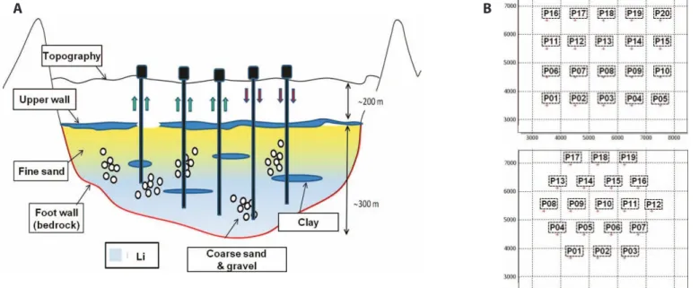
The deposit is a clastic reservoir, about 300 m thick, overlying an impervious bedrock. It is located 200 m under the surface. Figure 1a shows a west–east vertical cross-section. The project is at the feasibility stage where a risk analysis must be conducted to decide if the production should start and the first stage concerns the extractable grades, the porosity and permeability having been determined by pumping tests. The first analyses conducted by hydrogeologists lead to scenarios of future production drill holes where the predicted 40 year production curves must be calculated. Figure 1b shows two

configurations. Here, the aim is to quantify the impact of the grade uncertainty on the production curves and on the statistical distribution of the simulations.

Bailers

After drilling a hole for exploratory or future production purposes, the upper part of the hole is reinforced and cased while the deeper part – between a few metres and some hundred metres in length – is a filter that lets the brine pass through. After a few weeks, the brine inside the hole becomes stabilised and reflects the surrounding brine in terms of salt density and lithium grade (these variables are highly correlated). Then, a bailer – a plastic container that can be opened and closed by remote control – is introduced into the hole and opened at a given depth (measured by the length of the cable used) to capture the brine at this level (Figure 2). The bailer is recovered, its content sampled for future analyses (the lithium grade in our case), and reintroduced to sample a deeper level because all the brine between the sampled level and the surface is perturbed by the passage of the bailer. To evaluate the range of variation of the bailer fluctuations, some

FIG 1 – (A) West–east vertical cross-section scheme of a salar; (B) two configurations of future production drill holes.

A

B

measurements are replicated two or three times, with a few weeks interval.

We have at our disposal a first set of 100 measurements of grades in seven drill holes (Figure 3a). They sample elevations between 3250 m and 3550 m, representing the whole deposit. In this data set, 50 measurements are pairs located at the same place and finally, there are only 75 3D spatial locations involved. This first data set will be used for the geostatistical modelling and the grade simulations.

A second data set is at our disposal, symbolising complementary measurements made while the geostatistical study is done, a situation which often occurs. We use it for a statistical reconciliation, as shown in the following. In the future, one could imagine incorporating such complementary

measurements in the geostatistical study. The second data set contains replicates located at different places and/or measured at different times, giving 50 differences on which a pure statistical analysis is conducted to reconcile them with the nugget effect encountered in the variogram calculated with the first data set. As these measurements cover a domain larger than the domain of interest, the real comparison is made by using the 25 differences belonging, approximately, to the future production zone (Figure 3b).

geostatistical model for the grades

The scatter diagram between the grade and the elevation (Figure 4a) shows that the grade increases with the depth, which could be due to gravity segregation, since the salinity (well correlated to the lithium grade) leads to a fluid density that increases with depth up to values of around 1.2. The gradient is high: grades are multiplied by two after 300 m and this requires the use of non-stationary geostatistical techniques (Matheron, 1969) to model the spatial variability of the lithium grades.

A first approach could consist in fitting, by least squares, a linear trend to assess residuals supposed to be stationary. The idea is to apply universal kriging techniques (Matheron, 1969). But after fitting such a trend and looking at what is called ‘residuals’ (the grade value minus the trend model), one sees that if there is, on average, no remaining trend for the behaviour of the grades, this time the variance of the residuals is not stationary either (Figure 4b) and the variance (or more precisely its square root) must also be modelled. Note that the fact that low-grades fluctuate more than high-grades is unusual in mining and environment studies, where the reverse often happens and one usually says that there is a ‘proportional effect’ (Matheron, 1974). The decrease of variability with elevation is likely to be related to flow heterogeneity: the deepest, lithium-rich, part of the reservoir is made of rather coarse clastic material with good hydraulic conductivity, where flow is probably governed by regional gradients and gravity (high salt content). The upper part, as mentioned before, has a lesser lithium content. In this part of the reservoir, which extends to the surface, flow is governed by local recharge/discharge mechanisms. Finer materials and the presence of clay confer a lower hydraulic conductivity and, probably, a more heterogeneous velocity field. Between these two layers, a discontinuous clay layer marks the top of the reservoir. Complex mixing mechanisms around this discontinuous separation are the most probable causes of lithium concentration variations at the top of the reservoir. This is a very common characteristic of this type of deposit.

To account for the lack of stationarity, we set, for the lithium grade Li(x,y,z):

, , , ,

Li x y z^ h₌v^z NR x y zh ^ h₊m z^ h (1)

with

NR(x,y,z) the centred normalised residuals with the

variogram γ_NR(h)

σ(z) the standard deviation of the residual approximated by zvt^ h=a z bl + l

m(z) the trend approximated by m zt^ h=a z b+

The parameters a, b, a’, b’, are obtained by least squares minimisation and the simulation process (called ‘turning bands’, Matheron, 1973) consists in first simulating the normalised residuals NRS_{(x,y,z), conditionally to the}

experimental residuals obtained by:

FIG 3 – Horizontal cross-sections showing data location. (A) Crosses

represent the drill hole location where grades are measured, on average

eight measurements per drill hole at a fixed time plus between three

and four pairs of randomly selected duplicates per drill hole. (B) Black

dots represent the location of replicates to be statistically analysed for a

reconciliation with the geostatistical analyses conducted on the previous

data set (A). The small rectangular domain at the top corresponds to the

simulation domain. The entire domain is covered by 50 pairs of measurements

located at the same place in 3D (but measured at different periods), the

small rectangular domain reduces to 25 the number of differences.

A

S A SégUReT et al , , , , NR x y z Li x y z m z_z v = -t t t ^ ^ ^ ^ h h h h (2) and then rebuild the grades LiS_{(x,y,z) according to the formula:}

, , , ,

Li x y zS_{^ h=vt^}z NR x y z_h S_{^ h+}m z_{t^ h (3)}

The values are produced at the nodes of a fine grid (typically 40 m × 40 m × 1 m vertically). Each simulation reproduces the variogram model and the conditioning data. Each of as many simulations as wanted (100 in our case) represents a possible deposit. The variogram model depends on the trend model, the standard deviation model and the data set S that produced these parameters; they condition the simulations. In the following discussion we call the following set the ‘geostatistical model’:

, , , S m zt^ hvt^zhc_NR^hh

" ,: a geostatistical model (4)

UNCeRTAINTy OF The geOSTATISTICAL

mODeL

Among the 100 measurements at our disposal, 50 are fixed once and for all because they have not been replicated for unknown reasons, and 50 are duplicates measured at the same place but at different times. The question is how to choose the ones we must keep. We suppose that for each pair, the measurements are independent so that there is no reason to choose one value rather than another. To evaluate the impact of this uncertainty, the following procedure was applied: • for each of the 25 pairs of duplicates, randomly select one

value, and add to the 50 fixed values, producing a subset of 75 values

• repeat five times to produce five subsets S1...S5 of 75 values each

• for each subset S_i , calculate m zt_i^ h,vt_i^zh and γ_NRi(h)

• for each geostatistical model _"S m z_i, t_{i^ h},vt_i^z_h,c_NRi^h_h,,

conduct 20 geostatistical simulations

• for each simulation, which is a 3D grid of grades, apply a pumping simulation to evaluate the drainable resource • among the 100 simulations obtained, apply scenario

reduction techniques to find the five most representative simulations and determine if the bailer uncertainty has an impact on the distribution of the simulations.

The last two points will be treated in the following section. We now describe the geostatistical part.

Figure 4a shows the five lines m zt_i^ h obtained by least square

minimisations on the subsets S_i. They represent the average behaviour of the grade along the elevation. They are very close to each other and close to the line mt_all^ hz obtained by

using all the data. As we want a model as simple as possible, this sole drift mt_all^ hz will be subtracted from the grades to

calculate the residuals.

Figure 5a shows the lines vt_i^ hz fitted on the standard

deviations of the residuals. The differences this time are greater than previously, especially for the low elevations and we have to keep different standard deviation models for each subset. These models are used to divide the residuals and obtain the normalised residuals (Equation 2) on which the variograms are calculated. The horizontal variograms (Figure 5b) are approximately the same while the vertical ones (Figure 5c) can be grouped into two sets: a first one (S1,

S3, S4), leading to a local sill of around 0.5 and a nugget effect

of 20 per cent (compared to the global variance of 1), and a second set of variograms (S2, S5) leading to an apparent sill of 0.25 and a nugget effect of ten per cent. As for the standard deviations, each set S_i must have its own variogram model. Note the differences between the horizontal apparent sills (around 1.5) and the vertical apparent sills (less than 0.5), while the theoretical sill of normalised residual is 1 (around 1.1 in practice for all the subsets). This kind of ‘zonal’ anisotropy is another particularity of lithium grades in this type of deposits.

Conclusion:

• m(z) is robust as all the subsets lead to the same model

• σ(z) is less robust, one notices differences between the

models

FIG 4 – (A) Scatter diagram between the elevation and the lithium grades. The grades decrease with increasing elevation. Lines show the linear trends fitted by least

squares when using all the 100 measurements (including duplicates) or the five randomly selected subsets. The lines are almost identical. Black dots joined by dotted

lines represent averages by elevation classes, ie conditional expectation curve which is clearly linear. (B) Residuals obtained by calculating the differences between

the lithium grades and the line ‘All’ of Figure 4a. Surrounded stars are by pair the duplicates randomised. The variability of the residuals increases with the elevation.

• same for γ_NR(h), which leads to two different nugget

effects: ten per cent and 20 per cent.

Before proceeding to the following step (pumping simulation and scenario reduction), one must analyse in detail the nugget effects encountered in the variograms.

(geO)STATISTICAL ReCONCILIATION

Could the nugget effect encountered in the variograms, represent measurement errors, or, more generally, natural bailer fluctuations, meaning by ‘natural’ the possibility that the measurements might depend on the season, for example, something that we did not notice but which is still possible. The knowledge of the lithium industry is weak today, because until now no real investment has been made in deep research, as the profits are low. With prices that have been rising for a decade, it is probable that the situation will change soon and the present work is an indication of this tendency. At present, we do not have at our disposal continuous time series of grades over several years with which to calculate auto-correlations in time. This is why we speak of bailer ‘uncertainty’ and not necessary bailer ‘measurement errors’.

By their construction, the normalised residuals NR(x,y,z) have a mathematical expectation equal to zero, and a variance equal to 1, and we add the hypothesis that for each location

(x,y,z), all the replicates are independent of one another. In the

following, indices i and j represent statistical realisations of measurements (ie random samples).

By (1), a difference between two measurements in the same place is expressed by:

Δ_Li(x,y,z) = σ(z)Δ_NR(x,y,z) (5) Because E[NR_j(x,y,z)] is stationary and equal to zero, we have:

VAR[Δ_NR(x,y,z)] = E[(NR_i(x,y,z) – NR_j(x,y,z))2_]

= E[(NR_i(x,y,z)2_{] + E[(NR}

j(x,y,z)2] – 2E[NRi(x,y,z)NRj(x,y,z)]

Because VAR[NR(x,y,z)] is stationary, we have:

VAR[Δ_NR(x,y,z)] = 2E[(NR_i(x,y,z)2_{] – 2E[NR}

i(x,y,z)NRj(x,y,z)]

For each location (x,y,z), the independence of the random samples implies their non-correlation:

E[NR_i(x,y,z)NR_j(x,y,z)] = E[NR(x,y,z)]2

VAR[Δ_NR(x,y,z)] = 2VAR[NR(x,y,z)] = 2

A result, combined with (1), which gives, finally:

VAR[Δ_Li(x,y,z)] = σ2_(z)VAR[Δ

NR(x,y,z)] = 2σ2(z)

Let  represent the nugget effect of the normalised residuals variograms, expressed as a percentage of the sill. If the nugget effect is only due to bailer fluctuations, then, in the analyses of the statistical variances of type (5) differences, the following relationship must be verified:

, , Std dev x y z z 2Li a v D -= ^ ^ h h 6 @ ₍₆₎

We have at our disposal a second data set of measurements that covers a larger domain than the previous one (Figure 3b) and is essentially made of replicates (for some locations, the measurements are repeated up to four times), giving a set of

FIG 5 – (A) Linear modelling of the residual standard deviation as a function

of the elevation, depending on the data subset. Differences are large for low

elevations. (B) Horizontal variograms of the normalised residuals for each

data subset and all the data. Dotted line represents the normalised residuals

variance when all the data are used, it is close to 1 (1.1). (C) Vertical variograms

of the residuals for each data subset and all the data. For such small distances

(200 m), the vertical variograms have not reached the experimental variance.

A

C

B

S A SégUReT et al

50 differences Δ_Li(x,y,z) that we analyse to see if the results

are coherent with the experimental nugget effects. So the left-hand side of Equation 6 is built on this second data set, and we see the consistency with the right-hand one of (6), built on data file 1.

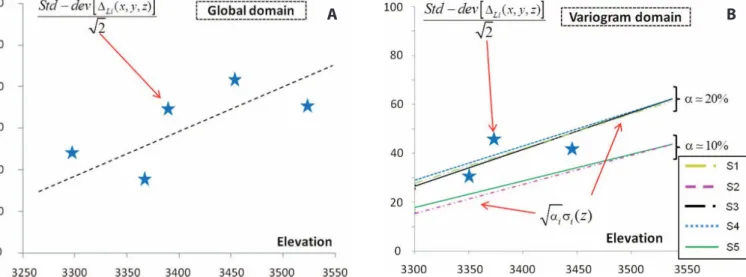
The first property of (6) is that the bailer fluctuations depend on the elevation. Is this true? Figure 6a presents the standard deviations of the differences grouped into four classes of elevations so that each blue star is calculated by around ten differences, and this is certainly too few. Nevertheless, the figure shows that the fluctuations increase significantly with the elevation.

Do they increase as a function of the standard deviation model? It becomes necessary to reduce the analysis to the domain covered by the variogram and other geostatistical parameters (Figure 3b), and this reduces the number of differences to 25. Figure 6b shows the three elevation classes (blue stars) obtained. Less than ten points for a robust estimation of a variance is hardly enough but, nevertheless, the figure shows that, for the models associated with a nugget effect close to 20 per cent, the results are coherent. They correspond to the geostatistical models S1, S3 and S4. Remember that we not only test a nugget effect value, but also a standard deviation model as shown by (6), as well as a drift model. For the two other sets, namely S2 and S5, associated with around ten per cent nugget, the coherence is not obtained.

Conclusions:

• it is possible to consider the nugget effect encountered in the residual variograms as due only to bailer fluctuations • the difficulty is to assess the correct value of the nugget

effect which must here be equal to 20 per cent

• for the future, a recommendation is made to the industrial partner to systematically make duplicates in order to thoroughly sample the bailer fluctuations all over the domain and not privilege unique data points over ones duplicated and randomly selected

• it is important to have a second data set made of replicates and different from the data set used for the models and the simulation as it may help to define the value of the nugget effect and eventually the models for m(z) and σ(z).

With each of the five geostatistical models (4), the simulation of the normalised residuals is conducted, conditionally to each subset S_i, and the grades are rebuilt using (3). Then, for each of the 100 equivalent deposits produced in this way, pumping simulations are made and scenario reduction carried out.

pUmpINg SImULATIONS

The challenge is now to simulate the lithium production, based on the concentration values obtained from the hundred geostatistical simulations, by a Finite Element modelling of the exploitation domain. The METIS code (Goblet, 2010), developed by the Geosciences Department and used in numerous studies of natural and artificial tracer simulations (Castro, Patriarche and Goblet, 2005), solves the equations of flow and solute transport in 3D space, taking into account the effect of density on flow. The hydrogeological parameters (conductivity and porosity) are attributed to the mesh cells according to a geological model built from field information. The main result obtained is the lithium production curve for each borehole. A set of representative curves are shown in Figure 7a for one specific simulation of lithium grades and the squared pumping scenario of Figure 1b.

In Figure 7b, the total amount of lithium recovered after 40 years of exploitation is shown for a set of 100 simulations. The five groups of 20 simulations do not exhibit a different behaviour in terms of average value and dispersion.

SCeNARIO ReDUCTION

Why reduce the number of possible scenarios? Over the past two decades, computer power has increased enormously, and it is now possible to generate hundreds of conditional geostatistical simulations for a deposit. The advantage of having a large number of simulations is that it provides a better idea of the potential upside and downside, and some simple calculations can be performed on these simulations. Unfortunately all the simulations that can be generated cannot be developed into economic studies. For example in the field of hydrocarbons, quite close to our case, post-processing involves complex fluid flow simulations with specialised software and also a large amount of engineer time to define the different architectures of infrastructures and finally the economic study. So our goal is to reduce the set of simulations to a more manageable size by selecting a representative subset

FIG 6 – (A) Bailer fluctuation along the elevation. The dotted line indicates the average tendency. The spatial domain concerns the whole salar.

(B) Reconciliation between the pure statistical analyses of the bailer fluctuations (data set 2, variances of the differences) and the spatial analyses

of the grades (data set 1, nugget effect of the variograms). For the conditioning data sets S1, S3 and S4, where the nugget effect α is around

20 per cent, the reconciliation is good; for the two other sets, where the nugget effect α is around ten per cent, the reconciliation is poor.

of them with a probability associated with each element of this subset. The size of the final subset is initially decided by the user. In general, it is the maximum number of simulations that can be post-processed with the available resources.

The two key elements in any scenario reduction method are: 1. defining a suitable indicator to measure the distance

between any two simulations

2. selecting the best subset of the predetermined size See (Armstrong, Ndiaye and Galli, 2010; Armstrong, 2012; Armstrong et al, 2013; Heitsch and Romisch, 2003) for more information of the methodology used and examples in mining.

To illustrate the approach we give the following intuitive image. Consider each simulation as a point in a high dimensional space in which we can calculate the distances between simulations. Note that these distances must be related to the work goal after the scenario reduction. Keep in mind as well that the topology of the cloud ‘N geostatistical simulations’ is not the same as the ‘N flow simulations’ cloud even if in general they are related. It is also clear that the result depends on the dimensions of the space in which we immerse the simulations (the dimensions represent the information which is considered for each simulation) and the distance measure used.

We must also have in mind that the best subset ‘k’ simulations’ is not a subset of ‘k simulations’ extracted from the optimal set of k (k>k’) simulations.

To apply this methodology to the present case of lithium deposit, the information used is the yearly production of each of the 20 wells during 40 years, discretised in 52 time intervals. There are many ways to represent this information in a high dimensional space. Here we study only two of them, and two variants combining them:

1. We can represent a flow simulation by a vector of 20 × 52 points obtained by concatenating the production of each well. This is CASE 1.

2. As it is often interesting to compute the total cumulated production versus the 52 time intervals, one might use only this information to represent the simulation. This is CASE 2 and the space dimension is only 52.

CASE 1 fully represents the variability of each one of 100 fluid flow simulations; it allows, for example, to take into account that some areas are special. The second representation, CASE 2, is more synthetic since the information of the 20 wells is summarised by a well with the total cumulative production. It is closer (although far more detailed) to the conventional method where one simply looks at the histograms of the total

output. We decided to combine the two approaches by using a distance matrix, which is the weighted average of the two preceding distance cases. In this case the space in which we are working is 20 × 52 + 52. We tested the cases where the distance matrix of CASE 1 is weighted by 0.8 (respectively 0.6) and the distance matrix of CASE 2 by 0.2 (respectively 0.4).

The result for CASE 1 is represented in Table 1.

It is instructive to calculate the average tonnage of the product after 40 years, obtained from the five best simulations using their probability computed while performing scenario reduction (Table 2).

The differences between the results are extremely small and the maximum relative error compared to the average of the 100 simulations is below two per cent. So with our five best simulations and probabilities we arrive at a very good estimate of the average of 100 simulations. This is, of course, not an absolute criterion, but the reduction process seems to work very well. However, note that the spread of the total productions of the 100 simulations (Figure 7b) is not very large. Moreover, the reduction scenario seems not to be sensitive to the fact that there are five sets of geostatistical simulations.

FIG 7 – (A) Simulated lithium recovery for a given lithium geostatistical simulation and squared scenario of Figure 1b. The cumulated amount

of lithium recovered at some production borehole is shown as a function of time. (B) The total amount of lithium recovered after 40 years for

a set of 100 simulations of lithium grades. No particular behaviour is visible for each subset (labelled S1 to S5) of 20 simulations.

A

B

CASE 1

CASE 2 0.6 CASE 1 + 0.4 CASE 2 0.8 CASE 1 + 0.2 CASE 2

102% 99% 99% 99%

TABLE 2

Relative average computed with the five optimal simulations

using their associated probability; 100 per cent corresponds

to the average of all initial (100) simulations.

Best simulations

Associated probability (%)

Percentile (%)

Geostatistical model

TABLE 1

Results of scenario reduction for CASE 1. The first line gives the optimal

simulation numbers; the second one the probability associated with

each simulation, for further computations; the third one indicates the

percentile corresponding to each optimal simulation in the initial set of

CONCLUSIONS

Classifying the drainable resources of a salar-type lithium deposit requires relating the geostatistical 3D simulations of grades to hydrogeological simulations (to quantify the metal extracted by pumping) and to scenario reduction (to find the most representative simulations among the hundreds or thousands produced). In this paper, we have focused on the grade uncertainty when measured by bailers.

The problem here is complicated by the lack of stationarity of grades that not only strongly increase with depth, but also fluctuate differently, depending on the elevation. So a geostatistical model is not only a variogram, but also a drift and a standard deviation model.

We have shown how the bailer fluctuations influence the geostatistical model. Five equivalent models were also evaluated, and their essential difference was their nugget effect values: three models lead to a nugget effect of around 20 per cent, two to ten per cent. By using an auxiliary data set made of replicates, it was possible to show that 20 per cent is the value that must be retained if the user wants just one model. In our case, the five models were tested along the complete methodological chain. Whether one considers the pumping results, or the scenario reduction, the fluctuations of the geostatistical models have no impact, and any of the models can be used to conduct the simulations.

In conclusion, we recommend systematic duplication of each measurement at all locations, so that sensitivity analyses can be conducted as done here. Then, the rudimentary bailer measurements can be used to carry out robust drainable resources estimations and classifications.

ACKNOWLeDgemeNTS

Due to confidentiality constraints that we understand, it is not possible to name here our friends, the geologists who provided us the original data that inspired the present synthetic case study. We warmly thank them, as well as three anonymous reviewers and a professional translator.

ReFeReNCeS

Armstrong, M, 2012. Scenario Reduction Applied to Mining (Geostatistical Association Australia: Perth).

Armstrong, M, Ndiaye, A A and Galli, A, 2010. Scenario reduction in mining, presented at IAMG Annual Meeting, Budapest, 29 August – 2 September 2010.

Armstrong, M, Ndiaye, A A, Razansimba, R and Galli, A, 2013. Scenario reduction applied to geostatistical simulations, Mathematical Geosciences, 45(2):165–182, doi: 10.1007/s11004-012-9420-7.

Castro, M C, Patriarche, D and Goblet, P, 2005. 2-D numerical simulations of groundwater flow, heat transfer and 4He transport – implications for the He terrestrial budget and the mantle helium-heat imbalance, Earth and Planetary Science Letters, 237(3– 4):893–910, doi: 10.1016/j.epsl.2005.06.037.

Garrett, D E, 2004. Handbook of Lithium and Natural Calcium Chloride: Their Deposits, Processing, Uses and Properties, first edition, 488 p (Elsevier: Amsterdam).

Goblet, P, 2010. Programme METIS – Simulation d’écoulement et de transport miscible en milieu poreux et fracturé – Notice de conception mise à jour le 6/09/10, Rapport Technique R100907PGOB, Centre de Géosciences, Ecole Nationale Supérieure des Mines de Paris, Fontainebleau.

Heitsch, H and Romisch, W, 2003. Scenario reduction algorithms in stochastic programming, Computational Optimization and Applications, 24:187–206.

Matheron, G, 1969. Le krigeage Universel, Cahiers du Centre de Morphologie Mathematique de Fontainebleau, Fasc. 1, Ecole des Mines de Paris, Fontainebleau.

Matheron, G, 1973. The intrinsic random functions and their applications, Advances in Applied Probabilities, 5(3):439–468, doi: 10.2307/1425829.

Matheron, G, 1974. Effet proportionnel et lognormalité: le retour du serpent de mer, technical report N-374, Centre de Geostatistique, Ecole des Mines de Paris, Fontainebleau.

Mohr, S H, Mudd, G M and Giurco, D, 2010. Lithium resources and production: a critical global assessment, report prepared for CSIRO Minerals Down Under Flagship by Department of Civil Engineering, Monash University Institute for Sustainable Futures, University of Technology, Sydney.