Millimeter-wave radar imaging systems : focusing antennas, passive compressive devicefor MIMO configurations and high resolution signal processing

(1)

HAL Id: tel-01933731

https://tel.archives-ouvertes.fr/tel-01933731

Submitted on 24 Nov 2018

HAL is a multi-disciplinary open access

archive for the deposit and dissemination of sci-entific research documents, whether they are pub-lished or not. The documents may come from teaching and research institutions in France or abroad, or from public or private research centers.

L’archive ouverte pluridisciplinaire HAL, est destinée au dépôt et à la diffusion de documents scientifiques de niveau recherche, publiés ou non, émanant des établissements d’enseignement et de recherche français ou étrangers, des laboratoires publics ou privés.

Millimeter-wave radar imaging systems : focusing

antennas, passive compressive devicefor MIMO

configurations and high resolution signal processing

Antoine Jouadé

To cite this version:

Antoine Jouadé. Millimeter-wave radar imaging systems : focusing antennas, passive compressive devicefor MIMO configurations and high resolution signal processing. Signal and Image processing. Université Rennes 1, 2017. English. �NNT : 2017REN1S154�. �tel-01933731�

(2)

ANNÉE 2017

THÈSE / UNIVERSITÉ DE RENNES 1

sous le sceau de l’Université Bretagne Loire

pour le grade de

DOCTEUR DE L’UNIVERSITÉ DE RENNES 1

Mention : Traitement du signal et Télécommunications

Ecole doctorale MathSTIC

présentée par

Antoine JOUADÉ

préparée à l’unité de recherche UMR-CNRS 6164, IETR

Institut d’Electronique et Télécommunications de Rennes

UFR Informatique et Electronique

Millimeter-wave

Radar Imaging Systems :

Focusing Antennas,

Passive Compressive Device

for MIMO conﬁgurations and

High Resolution

Signal Processing

Soutenance prévue à Rennes le 23 Novembre 2017

devant le jury composé de :

Marc LESTURGIE

Professeur, Centrale Supélec / rapporteur

Wolfgang MENZEL

Professeur, Université de Ulm / rapporteur

Hélène ORIOT

Maitre de recherche, établissement / examinateur

Atika MENHAJ

Professeur, Université de Valenciennes / examinateur

Olivier LAFOND

Maitre de Conférence HDR, Université de Rennes 1 / directeur de thèse

Laurent FERRO-FAMIL

Professeur, Université de Rennes 1 / Co-directeur de thèse

Mohamed HIMDI

Professeur, Université de Rennes 1 / Co-encadrant

Stéphane MÉRIC

(3)

(4)

On Feb 14, 1990 Voyager 1 looked back at Earth from a distance of 3.7 billion miles and took a picture... The image is known as the "Pale Blue Dot." We succeeded in taking that picture, and, if you look at it, you see

a dot. That’s here. That’s home. That’s us. On it, everyone you ever heard of, every human being who ever lived, lived out their lives. The aggregate of all our joys and suﬀerings, thousands of conﬁdent religions, ideologies and economic doctrines, every hunter and forager, every hero and coward, every creator and destroyer of civilizations, every king and peasant, every young couple in love, every hopeful child, every mother and father, every inventor and explorer, every teacher of morals, every corrupt politician, every superstar, every supreme leader, every saint and sinner in the history of our species, lived there – on a mote of dust, sus-pended in a sunbeam.

The Earth is a very small stage in a vast cosmic arena. Think of the rivers of blood spilled by all those generals and emperors so that in glory and in triumph they could become the momentary masters of a fraction of a dot. Think of the endless cruelties visited by the inhabitants of one corner of the dot on scarcely distinguishable inhabitants of some other corner of the dot. How frequent their misunderstandings, how eager they are to kill one another, how fervent their hatreds. Our posturing, our imagined self-importance, the delusion that we have some privileged position in the universe, are challenged by this point of pale light. [...] To my mind, there is perhaps no better demonstration of the folly of human conceits than this distant image of our tiny world. To me, it underscores our responsibility to deal more kindly and compassionately with one another and to preserve and cherish that pale blue dot, the only home we’ve ever known.

(5)

(6)

List of Figures

2.1 A geometric representation using the polar coordinate (d, θ, φ) from

the Cartesian coordinate (x, y, z). . . . 10

2.2 (a) Point-like targets location, (b) received signal in the spatial

do-main after range focusing. . . 14

2.3 Received signal in the spatial domain after range focusing and (a)

Hamming amplitude tapering and (b) Hanning amplitude tapering. . 14

2.4 Mechanically beam-scanning antenna solutions with in (a) the overall system is steered, in (b) only the feeder is steered and ﬁnally in (c)

only the focusing aperture is steered. . . 17

2.5 (a) Active system developed by JPL [6] with measurement results [25]

in (b) for diﬀerent target scenario for through-jacket of a mock pipe

bomb. . . 18

2.6 (a) Mechanically rotated reﬂect array with horn [26] with (b) an

ex-ample of the image reconstruction. . . 19

2.7 Electronically beam-scanning antenna solutions. . . 20

2.8 (a) Structure of the phased array [27] with (b) the beam scanning

capability. A measurement result is shown in (c). . . 22

2.9 Frequency beam-scanning antenna solution. . . 24

2.10 (a) The printed progressive wave antenna [31] with (b) and (c) the

beam scanning capability. . . 24

2.11 (a) Sar conﬁguration with (b) a 2D measured image and (c) a 3D

measured image. [36] . . . 27

2.12 SAR system mounted on a van at 300 GHz in (a) with in (b) the

imaging result and in (c) the optical image. [37] . . . 28

2.13 In (a) and (b) are shown the MIMO aperture conﬁguration with in

(c) the scene with the imaging result. [38] . . . 29

3.1 (a) A multi-dielectric Fresnel Zone plate lens [7] with in (b) the

cor-responding focusing gain. (c) A grooved Fresnel Zone plate lens [8]

with in (d) the corresponding focusing gain. (c) A perforated

(9)

LIST OF FIGURES

3.2 Sectional and top views of the ﬂat Fresnel lens with F the focal

dis-tance, D the diameter of the lens, d the thickness of the lens. θi yields

for a particular angle of incidence with the corresponding refracted

angle θt. The variable ∆ corresponds to the phase shift that occurs

at the input of the lens due to the spherical wavefront. . . 38

3.3 Phase shift that occurs at 75 GHz along the circular aperture diameter due to the spherical wave front and the generated phase compensation

using the ﬁve cases. . . 40

3.4 Phase compensation eﬃciency of the ﬁve cases versus the normalized

frequency band. . . 40

3.5 Theoretical aperture eﬃciency over the amplitude weighting

gener-ated by a cosn_{-like radiation pattern.} _{. . . 41}

3.6 (a) Sketch of the elliptical horn antenna and (b) the manufactured elliptical horn with rectangular-to-circular transition producing an

axially symmetric cosn_{-like radiation pattern} _{. . . 42}

3.7 Simulated and measured radiation pattern of the feeder at 90 GHz . . 42

3.8 Measured (Co/Cross polarization) radiation pattern of the optimized

feeder along the E (φ = 90◦_{) / H (φ = 0}◦_{) / 45}◦ _{(φ = 45}◦_{) planes}

com-pared with the associated cosn_{-like radiation pattern at the extreme}

frequencies (a) 75 GHz and (b) 110 GHz. . . 43

3.9 Oblique wave propagation through N layers of dielectric slabs with

mathbf E and mathbfH the electric and magnetic ﬁelds, respectively. 44

3.10 Comparison of the determined permittivity variation along the

diam-eter of the 2 circular lens apertures. . . 46

3.11 Variation of the transmission coeﬃcient along the diameter and versus

the considered frequency range for the (a) smooth and (b) smoothh

2πi

cases. (c) Variation of the transmission coeﬃcient eﬃciency versus the

considered frequency range for the two cases. . . 47

3.12 Simulated Electric ﬁeld (at 90 GHz) at the output of (a), (c), (e) the

smooth lens and (b), (d), (f) the smooth[2π] lens with a diameter of

12 cm; (a), (b) show the variation of the permittivity over the lens surface, while (c), (d) show the normalized electric ﬁeld distribution in amplitude (dB) over the lens surface and (e), (f) show the electric

ﬁeld distribution in phase (◦_{) over the lens surface.} _{. . . 49}

3.13 Initial thickness along the aperture diameter of each sub-lens before

being pressed. . . 50

3.14 Manufactured sub-lenses before pressing them for the (a) smoothh

2πi

and (b) smooth cases. . . . 50

3.15 Manufactured sub-lenses for the (left side) smoothh

2πi

and (right

(10)

LIST OF FIGURES

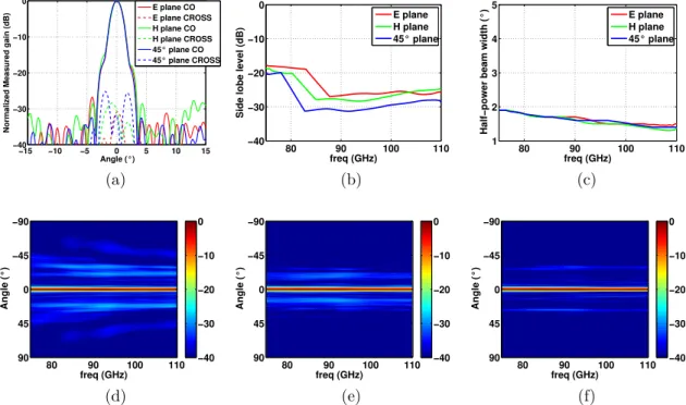
3.16 Measured radiation performance of the smooth lens. (a) radiation

pattern along the E/H/45◦ _{planes at 90 GHz. (b) Side lobe level}

along the E/H/45◦ _{planes versus the frequency range. (c) Half-power}

beam-width along the E/H/45◦ _{planes versus the frequency range.}

(d) Normalized E-plane radiation pattern (Co-polarization) versus the frequency range. (e) Normalized H-plane radiation pattern

(Co-polarization) versus the frequency range. (f) Normalized 45◦_-plane

radiation pattern (Co-polarization) versus the frequency range. . . 51

3.17 Measured radiation performance of the smoothh

2πi

lens. (a) radiation

pattern along the E/H/45◦ _{planes at 90 GHz. (b) Side lobe level}

along the E/H/45◦ _{planes versus the frequency range. (c) Half-power}

beam-width along the E/H/45◦ _{planes versus the frequency range.}

(d) Normalized E-plane radiation pattern (Co-polarization) versus the frequency range. (e) Normalized H-plane radiation pattern

(Co-polarization) versus the frequency range. (f) Normalized 45◦_-plane

radiation pattern (Co-polarization) versus the frequency range. . . 52

3.18 Simulated directivity and measured gain versus the frequency range for the smooth[2π] and smooth cases. The results are compared with the theoretical directivity optained by a uniform amplitude and phase aperture of same physical dimension than the manufactured lenses. The results are also compared to a uniform phase aperture with

am-plitude weighting generated by a cosn_{-like feeder radiation pattern}

with n lying between 35 and 70. . . 53

3.19 Simulated aperture eﬃciency for the smooth[2π] and smooth cases

versus the frequency. . . 53

3.20 Measured loss eﬃciency for the smooth[2π] and smooth cases versus

the frequency. . . 54

3.21 Measured total eﬃciency for the smooth[2π] and smooth cases versus

3.22 Schematic of the measurement setup. . . 57

3.23 Google map of the outdoor scene with (x), the location of the Direct radar imaging, (1), the building, (2), the old tractor, (3), the antenna

support and (4) the bruches and tall grass . . . 58

3.24 Measurement results with (a) the RAR image and (b) the RAR image

superposed to the Google map picture of the scene. . . 59

4.1 The diﬀerent indirect radar imaging conﬁgurations. . . 64

4.2 Scheme of the Near-ﬁeld/Far-ﬁeld transition . . . 67

4.3 Simulated results using a linear array with Nx = 10 and ∆x = 1λ,

with the dashed blue line corresponding to the element radiation pat-tern, the red line corresponding to the array factor and the black line

the array radiation pattern with a digitally beam scanning (a) θ0 = 0◦

(11)

LIST OF FIGURES

4.4 Simulated results using a linear array with Nx = 10, with the dashed

blue line corresponding to the element radiation pattern, the red line corresponding to the array factor and the black line the array

radia-tion pattern with (a) ∆x = 0.5λ, (b) ∆x = 1λ and (c) ∆x = 2λ. . . . 70

4.5 Simulated results using a square array with Nx = Ny = 10 and ∆x=

1λ and ∆y = 2λ, with (a) the element radiation pattern, (b) the array

factor and (c) the array radiation pattern. . . 71

4.6 MIMO conﬁguration (Tx: transmitting antenna location and Rx: rei-ceiving antenna location) used to generate a (a) fully populated linear

virtual array, (b) and (c) a fully populated virtual array. . . 72

4.7 Geometry of the radar imaging conﬁguration. . . 73

4.8 Simulated result of (a) the back-projected signal of the first receiving antenna, (b), the final SAR image after back-projection, (c) the final SAR image when the 2D Hamming tapering function is applied and (d) the final SAR image when the 2D Hanning tapering function is

applied. . . 76

4.9 Measurement setup.. . . 77

4.10 Picture of the three scene conﬁgurations with (a) 50 bolts of 5mm diameter conﬁgured to spell IETR,(b) a screw clamp, and (c) a knife

hidden inside a thick book. . . 78

4.11 SAR image results considering the scene with (a) bolts conﬁgured to

spell IETR, (b) the screw clamp and (c) the knife hidden in a book. . 78

4.12 Cutting view drawing of the 1x4 passive device with associated

trans-fer functions . . . 82

4.13 Exploded view drawing of the passive device with 1) the lower part with 2) the input and 3) the output ports. In 4) the diﬀractive element at the center of the cavity and in 5/6) the upper parts to close the

cavity. . . 82

4.14 Photography of (a) the output face of the realized passive compressive device, which works at millimeter-wave, and (b) the output face of

the horn antenna module. . . 84

4.15 Details of the antenna module with (a) Exploded view drawing of the horn antenna module with 1) the lower part, 2) the input ports attached to the output ports of the passive compressive device and (3) the upper part. The measured radiation pattern of the ﬁrst port

along (b) the E-plane Co-polar and (c) H-plane Co-polar (G(θ, f)). . 85

4.16 Absolute value in dB of the measured transfer functions by means of

a VNA along the frequency band. . . 86

4.17 The auto/cross-correlation results, rij(τ) = DF T−1[hi(f)hj(f)∗],

be-tween the measured transfer functions (VNA measurements), with the time domain τ (ns) along the horizontal axis and the normalized amplitude (dB) along the vertical axis. It is normalized by the

max-imum peak of the auto-correlation fonctions. DF T−1 _{yields for the}

(12)

LIST OF FIGURES

4.18 Measured power eﬃciency of the passive device corresponding to the outgoing powers from the four ports versus the incoming power along

4.19 Setup measurement using a Compact Antenna Test Range. . . 88

4.20 Sketch of the phase variation that occurs when the DUT is looking

at (a) broadside and (b) at squint angle. . . 90

4.21 Measured data along (b) the frequency domain and azimuth axis and

along (a) the azimuth axis at the ﬁrst frequency f + fc = 50GHz. . . 91

4.22 Measured data at f + fc = 50 GHz in (a) amplitude and (b) phase.

The black line corresponds to the measured data (Sr(θ, f)) and the

dashed red line corresponds to the result of the data model using the

estimated transfer function found from minimization (ˆSr(θ, f)). . . . 92

4.23 The auto/cross-correlation results, rij(τ) = DF T−1[hi(f)hj(f)∗],

be-tween the measured transfer functions (h(f)) and the estimated

trans-fer functions (ˆh(f)), with the time domain τ(ns) along the horizontal

axis and the normalized amplitude (dB) along the vertical axis. It is normalized by the maximum peak of the auto-correlation fonctions.

DF T−1 _{yields for the inverse discete Fourier transform.} _{. . . 93}

4.24 Absolute value of the complex inner product results between the mea-sured transfer functions (h(f)) and the estimated transfer functions

(ˆh(f)), along the frequency. . . . 93

4.26 Scene in the anechoic chamber composed of two corner reﬂectors. . . 96

4.27 Measurement imaging results, by using 4.30, of two isotropic targets (corner reﬂectors) captured by (a) a classic SIMO conﬁguration with 1Tx (transmitting element) and 40 Rxs (receiving elements), (b) the passive compressive device with 10 Rxs elements where the Port-to-Port measurement is used to have the transfer function and (c) the passive compressive device with 10 Rxs elements where the

plane-wave estimation is used to have the transfer function. . . 97

4.28 Schematic of the stacked patch antenna . . . 98

4.29 Feeding network dimension of the array of eight elements.. . . 100

4.30 Simulated S-parameter of one single element and an array of 8 elements.100

4.31 Simulated Co/Cross radiation pattern of the element along (a) the

E-plane and (b) the H-plane.. . . 101

4.32 Simulated Co/Cross radiation pattern of the passive array along (a)

the E-plane and (b) the E-plane. . . 102

4.33 Single element with (a) the fabricated prototype and (b) the exploded

view. . . 103

4.34 Passive array of 8 elements prototype . . . 103

4.35 Simulated and measured S-parameter of (a) the single element and

(b) the array of 8 elements. . . 104

4.36 (a) schematic drawing and (b) the manufactured Active array layout

of 8 independant elements. . . 106

(13)

LIST OF FIGURES

5.2 Sketch of the propagation of the range resolution front for a point-like target in a (a) far-field narrow-band configuration, (b) far-field wide-band configuration,(c) field narrow-wide-band configuration,(d) near-field wide-band configuration. The blue dots represent the extreme sides of the aperture represented by the dashed line. The arrow gives

the angle of incidence of the wave. . . 117

5.3 Simulation results of the matrix S for a point-like target in a far-ﬁeld narrow-band conﬁguration after (a) the range focusing and (c) the range and the cross-range focusing (Fourier SAR image without

compensations). (b) shows the phase variation along the aperture. . . 118

5.4 Simulation results of the raw data matrix S in the far-ﬁeld wide-band conﬁguration (a), (c), (e) without the wide-band compensation and (b), (d), (f) with the wide-band compensation. The results in (a) and (b) are shown after the range focusing and (e), (f) after the range and the cross-range focusing (Fourier SAR image). In (c) and (d) are

shown the phase variation along the aperture after the range focusing. 120

5.5 Simulation results of the raw data matrix S in the near-field narrow-band configuration (a), (c), (e) without the near-field compensation and (b), (d), (f) with the near-field compensation. The results in (a) and (b) are shown after the range focusing and (e), (f) after the range and the cross-range focusing (Fourier SAR image). In (c) and (d) are

shown the phase variation along the aperture after the range focusing. 121

5.6 Simulation results of the raw data matrix S in the near-field wide-band configuration after (a), (d), (g) the range focusing and after (c), (f),(i) the range and the cross-range focusing (Fourier SAR image). In (b), (e) and (h) are shown the phase variation along the aperture after the range focusing. In (a), (b), (c) no compensation occurs. In (d), (e), (f), only the wide-band compensation is applied and finally in (g), (h), (i), the near-field and the wide-band compensations are

applied. . . 122

5.7 Imaging geometry of the synthetic aperture Radar with the received

raw data focused over (a) a 2D Cartesian grid (b) a 2D polar grid. . . 123

5.8 Cutting views of the Imaging geometry showing the variation of (a) the range resolution along the plane considered (b) the azimuth

an-gular resolution along the range of observation angles. . . 125

5.9 Simulation results of the raw data matrix S after applying the focusing technique in the near-ﬁeld wide-band conﬁguration. The raw data is projected over (a), (c), (e), (g) a Cartesian grid (see Fig. 5.7a) and over (b), (d), (f), (h) a polar grid (see Fig. 5.7b) after (a), (b) the range focusing, after (g), (h) The range and the cross-range focusing (Fourier SAR image). In (c) and (d) are shown the phase variation after the range focusing and (e), (f) shows the 2D spectrum of the

reconstructed image. . . 126

5.10 (a) 1D (b) 2D Spatial smoothing applied on the irregular grid. . . 131

5.11 Flow chart of applying the spectral analysis algorithms in a near-ﬁeld

(14)

LIST OF FIGURES

5.12 Simulated results of 2D spectral estimation methods using (a), (b), (c), (d) a Cartesian grid and (e), (f), (g), (h) a polar grid with (a), (e) the beamforming method, (b), (f) spatial smoothed beamforming,

(c), (g) the CAPON method and (d), (h) the MUSIC method. . . 132

5.13 Imaging conﬁgurations with the two closely spaced point scatterers

located in the broadside angle area I and the squint angle area II. . . 133

5.14 1D spectral estimation methods applied along cross-range direction on the (a), (b), (c) broadside angle area I and (d), (e) (f) squint angle area II. (a), (d) show the beamforming method, while (b), (e) show the CAPON method and (c), (f) show the MUSIC pseudo-spectra

method. . . 134

5.15 2D spectral estimation methods applied on the (a), (b), (c) broadside angle area I and (d), (e) (f) squint angle area II. (a), (d) show the beamforming method, while (b), (e) show the CAPON method and

(c), (f) show the MUSIC pseudo-spectra method. . . 134

5.17 Picture of the three scene conﬁgurations with (a) 50 bolts of 5mm diameter conﬁgured to spell IETR,(b) a screw clamp, and (c) a knife

hidden inside a thick book. . . 136

5.18 2D spectral estimation methods applied on the (a), (d), (g), (j) bolts conﬁgured to spell IETR; (b), (e), (h), (k) the screw clamp and (c), (f), (i), (j) the knife hidden in a book. (a), (b), (c) show the beam-forming method and (d), (e), (f) show the beambeam-forming method after spatial smoothing, while (g), (h), (i) show the CAPON method and

(j), (k), (l) show the MUSIC methods. . . 137

5.19 2D spectral estimation methods applied on the imaging results (Carte-sian grid) using the MIMO conﬁguration with the passive compressive device considering (a), (e), (i), (m) one output, (b), (f), (j), (n) two outputs, (c), (g), (k), (o) three outputs and (d), (h), (l), (p) four outputs of the passive compressive device. (a), (b), (c), (d) show the beamforming method result and (e), (f), (g), (h) show the beamform-ing method result after spatial smoothbeamform-ing, while (i), (j), (k), (l) show the CAPON method result and (m), (n), (o), (p) show the MUSIC

method result.. . . 139

5.20 2D spectral estimation methods applied on the imaging results (Po-lar grid) using the MIMO conﬁguration with the passive compressive device considering (a), (e), (i), (m) one output, (b), (f), (j), (n) two outputs, (c), (g), (k), (o) three outputs and (d), (h), (l), (p) four outputs of the passive compressive device. (a), (b), (c), (d) show the beamforming method result and (e), (f), (g), (h) show the beamform-ing method result after spatial smoothbeamform-ing, while (i), (j), (k), (l) show the CAPON method result and (m), (n), (o), (p) show the MUSIC

method result.. . . 140

A.1 Synoptic of a pulsed RADAR . . . V

(15)

LIST OF FIGURES

A.3 Synoptic FMCW RADAR . . . IX

A.4 Instantaneous frequency . . . X

B.1 (a) eﬃcacité de compensation de phase, (b) eﬃcacité d’illumination de la lentille, (c) variation de permittivités nécessaire des lentilles, (d) les lentilles réalisées et (e), (f) résultats de mesures du système

antennaire.. . . XVI

B.2 Résultats des mesures radar avec (a) le système radar utilisé et (b), l’image radar et (c) l’image radar superposée avec une image de la

scène pris grâce à google map. . . XVII

B.3 Résultats de mesures pour trois diﬀérentes scènes. . . XVIII

B.4 Dispositif compressif passif. . . XIX

B.5 Flow chart of applying the spectral analysis algorithms in a near-ﬁeld

environment with wide-band signals. . . XX

B.6 Resultats des méthodes d’estimation spectrales (Beamforming, Beamofrm-ing avec "spatial smoothBeamofrm-ing", CAPON et MUSIC) 2D appliqué sur une scène avec un couteau caché dans un livre.2D spectral estimation

(16)

List of Tables

2.1 The main techniques . . . 8

2.2 Classiﬁcation of antenna parameters. . . 9

2.3 Evaluation of the diﬀerent direct techniques . . . 23

2.4 Evaluation of the indirect techniques . . . 30

3.1 Measured dielectric properties obtained from AIREX82 depending on the thickness ratio . . . 50

3.2 Summarized radiation performances for two lenses . . . 55

4.1 Summarized point spread function performances . . . 96

5.1 Simulation parameters for the different configurations (FF: Far-field, NF: Near-field, NB: Narrow-band and WB: Wide-band). . . 119

(17)

(18)

Chapter

1

Introduction

1.1 Context of study

The majority of the regions of the electromagnetic spectrum can be used for imaging the unseen. The diﬀerent operating frequencies provide various information about the area of interest that are interesting in many applications. The microwave op-erating frequencies enable to see at night, through clouds and some materials and thus provide a valuable supplement to other imaging techniques such as infrared or X-ray techniques.

The ability to distinguish small details of an object, also known as the spatial reso-lution, is directly linked to the frequency bandwidth used and the radiating aperture size of the device. At the visible frequencies, with a human eye having a pupil diam-eter of about 5 mm, the angular resolution is approximately equal to 0.0084◦_{. Such}

result corresponds to a spatial resolution of about 1 cm at a distance of 70 meter from the eye. To achieve the same resolution at microwave frequencies, an aperture length of 250 m at a frequency of 10 GHz is required which makes it rather difficult to realize. In order to obtain high resolution images even at microwave frequencies, one of the greatest advance is the principle of synthetic aperture thanks to a radar system embedded on a moving platform (satellite, plane, drone, ...). It has widely been used for the earth observation. For near-range applications such as automotive, concealed object detection under clothes and plenty of other applications, a more compact system working with real-time acquisitions is required. This is where the Synthetic Aperture Radar (SAR) technique reaches its limit because it is required that the area of interest is motionless during the travel path of the moving platform. To improve the resolution while keeping an acceptable size, increasing the fre-quency such as going at millimeter-wave is of great interest thanks to its reduced wavelength and wide frequency bands available. However, for real time acquisitions, it is needed to physically sample an aperture with a large number of antennas and associated chains (transmitter/receiver). Due to the small wavelength and then the small components size, the fabrication process complexity is increased as for the cost. Nowadays, main researches are concentrating their efforts to find solutions to reduce the number of chains while keeping an acceptable spatial resolution. Either

(19)

INTRODUCTION the sampling pattern over the aperture is studied or it is developed advanced signal processing techniques or tools to improve the spatial resolution.

Among all the methods allowing to improve the Radar imaging capability, the goal of this study is to investigate various solutions and techniques while keeping and improving the more relevant ones.

1.2 Thesis Organization

The thesis is organized around four main chapters:

The chapter 2 outlines the basic of radar followed by a brief state-of-arts on radar imaging systems. Two main radar configurations will be presented. First, the Real Aperture Radar (RAR), also known as the direct imaging technique. The main solu-tions to scan the beam of antennas to produce a radar image will be given. Second, the Synthetic Aperture Radar, also known as indirect imaging technique. Different modes of SAR may be used. The modes are listed and compared to determine the relevant one that will be deeper studied. Finally, the theory of the radar principle is studied and applied on simulated data to determine the achievable range resolution using frequency diversity. This chapter permits to select among the different meth-ods presented, the more relevant ones that will be further detailed or improved in the next chapters.

In the chapter 3 is further presented the Real Aperture Radar configuration, where the image is realized pixel by pixel using high directive antennas in which the main beam is scanned. A high directive Fresnel lens antenna is studied, simulated and measured. As compared to the literature in which the lens is sampled in multiple but limited zones, in this work, a smooth version is realized thanks to a new tech-nological process. As compared to other methods, the smooth version of the Fresnel lens leads to an improvement of efficiency and a stable gain over a wide frequency band. Finally, the Fresnel lens antenna will be used in a RAR configuration using only one couple of transmitter (Tx) and receiver (Rx) chains to generate a radar image of an outdoor scene using a mechanically beam scanning capability. However, this solution reaches its limit when real-time radar imaging systems are necessary. In the chapter 4 is presented the SAR theory with the associated focusing algorithm required to generate the SAR image. Thanks to a scanner system, measurements are performed at millimeter-wave to create high spatial resolution SAR images of small objects such as a knife. The scanner synthesizes a receiving array of indepen-dent elements. When a real receiving array is used, a high number of Rx chains is required which leads to a complex and costly solution. To reduce the number of chains, the next study focuses on the use of a Multiple-Input-Multiple-Output (MIMO) configuration where the main goal is to reduce the number of chains by means of the virtual array theory. To further reduce the number of chains, a passive compressive device is studied, realized and measured, which has the capability to compress multiple signals into one while making each signal decorrelated from each other in a passive manner. Each channel inside the device is related to its own trans-fer function in the frequency domain. Two methods to measure or to estimate the transfer functions with great accuracy are studied. Finally, the passive compressive

(20)

INTRODUCTION

device is used in a MIMO conﬁguration showing the great capability of the passive compressive device to reduce the number of chains while maintaining unchanged the spatial resolution.

In the previous chapter, it is shown how it is possible to reduce the number of Tx and Rx chains while maintaining unchanged the spatial resolution by modifying the geometry of the transmitting and receiving antenna array. In the chapter 5, from a limited number of elements (antennas and associated chains), the received signals are digitally processed by means of spectral estimation methods to improve the spatial resolution. The method is dedicated to specific configurations and assumptions are made such as the narrow band and the far-field configuration. A solution able to use spectral estimation methods in a near-field and wide-band configuration is shown. The solution is applied on real data showing the improved spatial resolution in a near-field and wide-band configuration.

Finally, the last chapter concludes the study and points to several directions for future researches to improve the spatial resolution while keeping as low as possible the number of Tx/Rx chains available.

(21)

(22)

Chapter

2

RADAR systems

Radar systems are used to detect the electromagnetic waves that propagates within a certain domain of space and to measure the electromagnetic responses. Three diﬀerent Radar systems may be used.

• Passive radar [1, 2]: The passive radar system detects the energy naturally emitted by the scene (naturally emitted black-body radiation). Because, the passive radar does not transmit any signals, it only requires receiving chains. However, one of the main drawback of a passive system, is that it is not possible to focus along the range axis which is a strong limitation for our goal.

• Passive radar using signals of opportunity [3–5]: Because in the elec-tromagnetic spectrum, frequency bands are already allocated for various ap-plications such as railway/maritime/aeronautical/spatial/military communi-cations, wireless multimedia communicommuni-cations, radiolocalisation and satellite navigation systems, radio astronomy, earth exploration, weather satellite, ac-tive radar and imaging Synthetic Aperture Radar applications, the passive radar system using signals of opportunity detects the backscattered signals coming from the applications listed above. Such a radar has the capability of operation without any spectrum resource allocation and a potentially null probability of being intercepted. It only requires receiving chains to acquire the backscattered signals. However, it is spatially limited by the coverage of the transmitter.

• Active radar [6, 7]: An active radar transmits its own signal over a limited frequency band through a certain domain of space and measure the electro-magnetic responses of obstacles, also called targets or scatterers. The system requires both transmitting and receiving chains.

A passive imaging system has the advantage to be simpler to implement because there is no need for a transmitter chain (use of free natural illumination). This kind of system is safe for humans because there is no illumination to human body. On the contrary, a passive system suﬀers from the problem of a small received power due to the thermal noise of the target. So the image contrast can be very low within a limited range of distance. If the application needs to extend the distance and increase

(23)

CHAPTER 2. RADAR SYSTEMS the received power, an active system is desirable even if the global implementation is more costly and complex. It has to be underlined that using active sensors and knowing the emitted signal, we are able to compare the emitted and received signals, and set up an improvement of the signal-to-noise ratio thanks to the matched ﬁlter and therefore improve the ability to analyze and detect the scene and the targets.

2.1 Frequency spectrum

In the past decades, we have witnessed an impressive development to extend the ca-pability of detection based on magnetic, acoustic, ultrasound, microwave, millimeter-wave, TeraHertz, infrared and x-ray sensors [8–11]. An overview of the diﬀerent imaging technologies available will be brieﬂy considered showing the most relevant techniques found in the literature.

• Infrared technique (3 THz - 300 THz) [12]: This technique is based on the detection of thermal radiations which is a function of the frequency and absolute temperature. In another word, the capability of detection of such a system depends on the temperature diﬀerence between the diﬀerent objects to be detected and the human body. When used for Concealed Weapon De-tections (CWD) operations, infrared imaging has some drawbacks. First of all, the short wavelength of infrared doesn’t permit to penetrate thick clothes. Another drawback is that as soon as the temperature of the object is close to the body’s one, the detection is impossible. This occurs when the object is kept under clothing for a long time.

• X-ray technique (300 PHz - 30 EHz) [13]: Medical screening is the main use of X-ray imaging thanks to its ability to penetrate body and clothes with high spatial resolution but certain studies have focused on concealed human detection inside a truck. The main drawback of this system is that X-ray radiation is ionizing and so, a dose is radiated toward human.

• Micro/millimeter-wave technique (3 GHz - 300 GHz) [14]: Millimeter waves are suitable for security surveillance and especially for the detection of objects concealed under people’s clothing and baggage. In fact, thanks to the short wavelengths (from 30 GHz (10 mm wavelength) to 300 GHz (1 mm wavelength)) which have the ability to penetrate dielectric materials such as plastic or cloth and are strongly reflected by metallic materials, it is able to pass through obscurants such as fog, cloud, smoke and night. Unlike X-ray, millimeter waves are non-ionizing and can be used to detect both metallic and nonmetallic objects. They can achieve high spatial resolution by going in higher frequencies but material and atmosphere attenuation also increase so a trade-off has to be addressed. Depending on the applications, we are able to define an optimal frequency which allow to detect and image a weapon for instance at 10 meter from the system.

• Terahertz technique (300 GHz - 3THz) [15, 16]: THz is also interesting because it allows to classify diﬀerent type of materials. In fact each material

(24)

CHAPTER 2. RADAR SYSTEMS

has a diﬀerent absorption spectra in THz frequency range. THz can be used for security screening but its applications is limited to a very short range 3D imaging.

The diﬀerent concealed weapon detection techniques are tabulated in the Ta-ble 2.1 showing their main advantages and issues but also the type of illumination, the possibility of penetration and also the distance of the imaging scene capability. MMW based technology has the widest range of possibility to make an imaging system. The system can be transportable and both metals and non-metals can be detected. Even though THz provides high resolution, it doesn’t permit to illuminate a large scene because of the high atmospheric absorption and its medium penetra-tion.

As explained before, infrared technique is not a suitable solution due to its low penetration which doesn’t fit the requirement. Moreover, this kind of systems is not able to differentiate targets having the same temperature. X-ray imager due to its safety concerns (ionizing radiation) hinders its acceptance to illuminate human body but this is also because of its low range of detection and imaging. The choice of MMW system is the most suitable solution to fit the requirement thanks to its good penetration ability and high resolution but also the capability of size reduction, wide available bandwidth and industrial interference frequencies which are really much weaker than those at microwave bands. In this frequency range, the electromagnetic wave penetrates most of dielectrics and it exists some particular and advantageous atmospheric windows (no additional absorption) allowing to implement imaging sys-tems for security and people protection.

For a near-range imaging system up to about 20 meters, the study will mainly focus on active systems working at millimeter-wave. As explained previously, the active system allows to detect targets farther while going through material such as detecting concealed objects under clothes. Furthermore, thanks to the small wave-length at millimeter-wave, it allows to manufacture active radar with an acceptable size.

2.2 Radar equation

Let consider an active radar having only one transmitting and one receiving chain with antennas in the front-end of the chains. A RF stimulus signal (Se(f)) with output power Pe is transmitted with a frequency diversity over a frequency band-width Bf with f ∈ [−Bf/2, Bf/2]. Before being sent through the medium, the signal has been transposed around the carrier frequency fc, with its counterpart in the spatial frequency domain (wavenumber domain) kc = 4π/λc = 4πfc/c and the

spatial frequency band k ∈ [−2πBf/c,2πBf/c]. The speed of light is set out with

c and λc corresponds to the wavelength at the carrier frequency fc. We note that

the expression of the wave number shows a factor of 2 as compared with common conventions. The transmitted signal will be delayed from the propagation from the transmitted antenna to a speciﬁc target and backscattered to the receiving antenna. It is because we are only interested in the one-way distance between the radar to

(25)

Table 2.1: The main techniques

Tech-nologies Illumi-nation Proxim-ity Pene-tration Main

advantages Main issues

Infrared Passive Far Low

Passive system and possible detection and imaging at far distance Low penetration and no diﬀerentiation when temperature contrast is low X-Ray Active Near Very-_high Allow to detect_{inside the body} Safety concernsand low

proximity MMW Activeor Passive Far High Resolution high enough to image concealed objects, good penetration, possible portable system high-cost (non-availability of components in high-frequencies, important atmospheric absorption at speciﬁc frequency bands)

THz Active Near Medium

High-spatial resolution and possible detection and separation of materials high-absorption lost, stand-oﬀ detection unsuitable, high atmospheric absorption

(26)

Table 2.2: Classiﬁcation of antenna parameters

Radiation properties Circuits properties Mechanical_properties

Radiation pattern (Directivity,

Beam width, Side lobe level) Impedance (matching) Type of antenna Radiation eﬃciency Frequency bandwidth Shape

Gain Size

Eﬀective area Mass

Aperture eﬃciency Phase radiation pattern Polarization of EM wave

Cross-Polarization

the target, that the factor two in the wavenumber arises. It will be useful when we will derive the data model.

2.2.1 Antenna parameters

An antenna is a device which converts circuit currents into propagating electro-magnetic waves and, by reciprocity, collects propagating electroelectro-magnetic waves and converts it into circuit currents. Several quantities may be deﬁned in order to de-scribe an antenna that are summarized in the Table 2.2.

In this section, a perfect antenna with an optimal eﬃciency and null cross-polarization level is considered. The maximum gain corresponds to the directivity and we are only concerned by the radiation pattern. When it is needed to display the radiation pattern of an antenna, it is more common to use a spherical reference. However, in the Section2.2.2, the conﬁguration that will be used is considered with respect to an orthogonal Cartesian reference. It is then required a Cartesian to spherical coordinate transformation. The transformation is shown in (2.1) using the Fig. 2.1.

For expressing the far-ﬁeld quantities, a spherical reference coordinate (d, θ, φ) is considered with θ ∈ [−π, π] measuring the rotation from the x − axis in the

xy_{− plane and with φ ∈ [0, π] measuring the tilting with respect to the z − axis.}

From a particular point Pi(xi, yi, zi), the transformation is given by (2.1).

xi = di cos θi sin φi

yi = di sin θi sin φi

zi = di cos φi

(2.1) In what follows, G(k, θ, φ) corresponds to the variation of the gain along the spatial frequency domain within the two angular sectors θ and φ. Here, k is the wavenumber variable directly linked to the frequency. The expression corresponds to the ratio between the surface density of the radiated power and that radiated by an isotropic antenna with a radiation pattern uniformly distributed on a sphere.

(27)

CHAPTER 2. RADAR SYSTEMS The angles θi and φi correspond to the look angles from the center of the spherical coordinates.

Figure 2.1: A geometric representation using the polar coordinate (d, θ, φ) from the Cartesian coordinate (x, y, z).

2.2.2 Conﬁguration

In a 3-Dimensional spatial space, a transmitting antenna is located at a fixed position with a gain variation Gt(k, θ, φ). The location of its phase center is (xt, yt, zt). The phase center of the receiving antenna is (xa, ya, za) with a gain variation Ga(k, θ, φ). It is considered Ns point scatterers which are identified by their Cartesian coordi-nates (xi, yi, zi). The index i yields for the ith point scatterer Pi with σi(k, θi, φi) the Radar Cross-Section (RCS) of the ith _{target over the frequency diversity. In this} situation, it is considered that the RCS of the target is a constant through time and look angles and variations only occur over the frequency band Bf. The one-way distance (corresponding to the radial distance) for the wave propagating from the transmitting antenna to the point scatterer Pi and then reflected back upon the receiving antenna is given by [17]:

di = 1

2(dT xi+ dRxi)

=q(xt − xi)2_{+ (yt} _{− yi)}2_{+ (zt}_{− zi)}2_/₂

+q(xa− xi)2 + (ya− yi)2+ (za− zi)2/2

(2.2)

The received signals, at the receiving antenna level, are modeled as a sum of transmitted signals that are weighted and delayed [18]. The complex weighting

si(k, θi, φi) represents all the attenuations that occur during the round-trip

(28)

is a characteristic of the observed scatterer and can be expressed as a function of the reﬂection coeﬃcient σi(k, θi, φi) = limdi→∞4π d

2

i|Es(di)|

2

|E0|2 with E0 that represents the

incident field on the scatterer and Es(di) is the amplitude of the reflected field from the scatterer at a distance di away from it. The interaction of the electro-magnetic wave with a scatterer can be briefly described by four elementary mechanisms: reflec-tion, refracreflec-tion, diffraction and scattering [19,20]. Considering that the look angles

θi and φi are similar (mono-static conﬁguration) for the transmitting and receiving antennas, the complex weighting can be modeled using the radar equation [21] in (2.3).

si(k, θi, φi) = PeGt(k, θi, φi) Ga(k, θi, φi) (2π)2

((k + kc)/2)2_(4π)3_d4

i

σi(k, θi, φi) (2.3) The delays arise from the round-trip distances determined in (2.2). Furthermore, a Gaussian white noise n(k) ∼ NC(0, σ2) with zero mean and variance σ2 is present.

The received signals can then be modeled as:

Sr(k) = Su(k) + n(k) = Ns

X

i=1

si(k, θi, φi) Se(k) e−j(k+kc) di+ n(k) (2.4) with Su(k) corresponds to the useful signals. The Gaussian white noise n(k) is a measurement noise with a noise power Pn, inherent to the use of electronic devices and random by nature. We measure the quality of the received signal through the ratio of powers associated with the useful component and the noise, called the Signal-to-Noise power Ratio (SNR). As the noise is considered as white on the eﬀective band (Bf) of the receiver, it has a spectral density with uniform power on this domain equal to Nn in W/Hz. A sampling of this signal at a frequency fs = Bf gives uncorrelated sampled with a variance equal to BfNn. The signal to noise ratio is

then derived as in (2.5).

SNR = si(k, θi, φi)

BfNn

(2.5) The radar system can be optimized to improve the SNR. Because we are con-sidering a radar working at millimeter-wave, the delivered output power remains relatively low (from -10 to 10 dBm in general). The RCS and the distance between the target and the radar are fixed parameters by essence. Then, in order to improve the SNR, it is only possible to increase the gain (more efficient antenna or more directive radiation pattern), in the desired look angles at the transmitting and re-ceiving levels. By doing so, this allows to improve the SNR of the systems but the field of view of the system will be reduced.

2.3 Range focusing using frequency diversity

From now, we have only received the backscattered signals but it is not possible to estimate the reﬂectivities and the distance di of the ith _{backscattered signal. Thanks} to the frequency diversity, it is possible to estimate the Ns targets range location

(29)

CHAPTER 2. RADAR SYSTEMS with the help of a suﬃcient number of frequency components. Considering τ as the time variable, we therefore use a waveform u(τ) with the bandwidth Bf adapted to the analysis of the observed scene.

In order to enhance, distinguish and extract the desired signal knowing that the receiver has the knowledge of the transmitted signal, the optimal filter, also called the matched filter, is performed on the received raw data [17]. When the noise affecting the measurement does not present a particular structure, in other words, when it is white, the filtering solution leading to an optimal SNR is given by gr(k) = S∗

e(k) with (·)∗ the complex conjugate operator. The function gr(k) is considered as the transfer function of the radar system. In the Appendix A.1 is shown the theoretical development to reach the optimal solution.

The impulse response in the time domain of the processing chain is then given by:

h(τ) =Z +∞

−∞ se(t)s ∗

e(t − τ)dt (2.6)

In Appendix A.2 is shown the theoretical development to reach the impulse re-sponse when a pulsed linear frequency modulated waveform (chirp) is used [22]. Using the Chirp waveform, it is required to sample the down-converted received signal at the frequency bandwidth used (Bf) with respect to the Shannon crite-rion. The expression of the radar impulse response for the pulsed linear frequency modulated waveforms is:

hc(τ) = τptri( τ 2τp) sinc(Bftri( τ 2τp)τ) ≈ τpsinc(Bfτ) (2.7) The approximation is valid if we consider Bfτp >> 1 with τp the pulse duration. After range focusing, the Signal-to-Noise Ratio is given by SNRf = TpfsSNR with

fs ≥ Bf the sampling frequency.

In Appendix A.3 is shown the theoretical development to reach the impulse re-sponse when an increasing linear frequency modulated continuous waveform is used. As compared to the Chirp waveform, using the FMCW waveform, the received sig-nal is directly demodulated by the transmitted sigsig-nal. The sampling is not linked to the frequency bandwidth used but by the slope of the linear frequency transmit-ted with fs ≥ Nf/Tp. After range focusing, the Signal-to-Noise Ratio is given by

SN Rf = TpfsSN R.

In AppendixA.4is shown the theoretical development to reach the impulse response when a stepped frequency continuous waveform is used. After range focusing, the Signal-to-Noise Ratio is given by SNRf = NfSN Rwith Nf the number of frequency

bins. hFMCW(τ) ≈ hSFCW(τ) = sin(πBfτ) sin(πδfτ) ≈ Nfsinc(Bfτ) (2.8) The approximation is valid if we consider Bf = δf(Nf _{− 1) ≈ δ}fNf with δf the step frequency. The range resolution that corresponds to the width of the main lobe at

(30)

CHAPTER 2. RADAR SYSTEMS -3 dB is:

δr =

c

2Bf (2.9)

The received signal in the frequency domain after applying the range focusing technique by adapted ﬁltering is expressed as:

S(k) = Sr(k)S_e∗(k) = H(k)

Ns

X

i=1

si(k, θi, φi) e−j(k+kc) di+ nf(k) (2.10)

where H(k) is the transfer function of the system in the wavenumber domain. The expression nf(k) = n(k) S∗

e(k) corresponds to the ﬁltered white noise by means of the matched ﬁltering technique.

The received signal in the spatial domain after an inverse Fourier Transform of (2.10) is expressed as:

s(d) =

Ns

X

i=1

si(d, θi, φi) h(d − di) e−jkcdi+ n(d) (2.11)

where h(d) is the impulse response in the spatial domain, with d, the radial distance or the range.

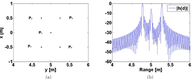
Considering a SFCW radar with a carrier frequency fc = 60 GHz and a fre-quency bandwidth Bf = 5 GHz which provides a transmitted power of 0 dBm, this corresponds to a range resolution δr= 3 cm. Both the transmitting and the receiv-ing antennas are located at the origin of the Cartesian coordinate (i.e. xt = xa = 0, yt = ya = 0, zt = za = 0). Both antennas have an isotropic radiation pattern

Gt= Ga = 0 dBi. In this example, there is no noise that corrupts the received sig-nals. In order to simulate targets, it is considered 5 point-like targets with uniform and time-invariant RCSs. For the simulation, it is considered that the weighting si is unitary and isotropic for i = {1, · · · , 5}. The location of each target is: P1(x1 =

−0.5 m, y1 = +4.75 m, z1 = 0 m), P2(x2 = +0.5 m, y2 = +4.75 m, z2 = 0 m), P3(x3 = 0 m, y3 = +5 m, z3 = 0 m), P4(x4 = −0.5 m, y4 = +5.25 m, z4 = 0 m), P5(x5 = +0.5 m, y5 = +5.25 m, z5 = 0 m) as shown in Fig. 2.2a for z = 0 m.

Because the distances of P1 and P2 to the radar are similar, both have the same

range which is also the case for P4 and P5. In Fig. 2.2b, it is shown the simulated

result of (2.11) after range focusing. Only three peaks are visible with the ﬁrst peak corresponding to the reﬂected signals from P1and P2, the second peak for P3and the

last peak for P4and P5. The highest Side Lobe Level (SLL) is -13.6 dB from the peak

lobes due to the impulse response that corresponds to a sinc-function. But, farther from the main lobe, the lower become the SLL. In order to reduce the highest Side-Lobe Level, it is possible to apply an amplitude tapering function on (2.10) such as Hamming or Hanning [23]. It drastically reduces the highest side lobes level. Nevertheless, due to the amplitude tapering, the eﬀective frequency bandwidth is also reduced inducing an increase of the range resolution. The amplitude tapering is a useful tool when the area of interest is in a near-range region. In fact, the strong coupling between the transmitting and reﬂecting antennas generates a strong peak at a distance corresponding to the distance between the antennas (or the strong

(31)

(a) (b)

Figure 2.2: (a) Point-like targets location, (b) received signal in the spatial domain after range focusing.

(a) (b)

Figure 2.3: Received signal in the spatial domain after range focusing and (a) Hamming amplitude tapering and (b) Hanning amplitude tapering.

reflection coefficient of the antenna if the measurement is performed using the same antenna in reflection mode (S11 measurements)). The side-lobes level of the strong

peak may hide the weaker backscattered signals (signals of interest). Applying an amplitude tapering reduces the side lobes level of the strong peak due to the antenna coupling allowing to extract the weaker desired signals.

The amplitude coeﬃcients of the hamming window is given by the following equation:

w(n) = 0.54 − 0.46 cos(2πn

N), 0 ≤ n ≤ N (2.12)

with the window length Nf = N + 1. The amplitude coeﬃcients of the hanning window is given by the following equation:

w(n) = 0.5(1 − cos(2πn

N), 0 ≤ n ≤ N (2.13)

(32)

CHAPTER 2. RADAR SYSTEMS focusing is given by:

sw(d) = 1

2π

Z +∞

−∞ w(k)S(k)e

jkd_dk _(2.14) In Fig. 2.3, it is shown the same simulated result as in Fig. 2.2bbut it is applied a Hamming and a Hanning amplitude taper function on (2.10). The highest side lobe level is -40.6 dB from the main peak lobe but farther from the main lobes, the SLL is slowly reduced. Furthermore, the range resolution has been increased with

δr = 4.5 cm for the Hamming function. For the Hanning function, the highest side lobe level is -30.6 dB from the main peak lobe but farther from the main lobes, the SLL is rapidly reduced with a slope similar to the uniform amplitude taper. Furthermore, the range resolution has been increased with δr = 5.05 cm.

2.4 State-of-art of Radar imaging systems

In the previous section, it has been shown the great capability of millimeter-wave for radar applications. It has been demonstrated through simulations that using only one pair of transmitting and receiving antennas, it is possible to estimate the location of targets only along the range direction (distance between targets and radar). Then, for targets having the same range from the radar perspective, it is not possible to resolve or separate the targets thanks to spectral diversity. In this section, two methods are shown to resolve and locate targets in range and cross-range directions in order to perform 2-Dimensional or 3-Dimensional Radar imaging, the Direct and Indirect imaging techniques.

• Direct Imaging technique: The technique uses spatial ﬁltering or

beam-forming thanks to the radiation pattern of the antenna that is scanned over

an area of interest. The half-power beam width gives the resolution of the sys-tem to discriminate targets along the cross-range direction. Then it is required a high-directive antenna to achieve great resolution. The scanning capability may be classiﬁed in three groups: Mechanically beam-scanning, Electronically beam-scanning and Frequency beam-scanning.

• Indirect Imaging technique: The technique uses spatial diversity or

dig-ital beamforming thanks to a group of independent antennas that acquires

the signals and by means of signal processing. The beam is digitally scanned by coherently combining in amplitude and phase the signals received by the independent antennas.

A state of art of imaging systems using both direct and indirect imaging tech-niques mainly used in the literature are presented to show advantages and draw-backs of the techniques. It is a general "state of the art" in which, the details of the antennas, the algorithms are not provided because these aspects are assessed and addressed in the next chapters.

(33)

2.4.1 Direct imaging

Plenty of conﬁgurations exist in the literature for direct imaging. Nonetheless, only the main conﬁgurations are detailed and compared in this section.

The antenna design is of major interest for the direct imaging in order to have an optimal Signal-to-Noise Ratio in the desired frequency bandwidth. The different types of antenna subject to the kind of beam-scanning chosen may be evaluated following the different parameters stated in the Table 2.2. At millimeter wave, five major criteria have to be considered:

• The overall eﬃciency: The gain of the antenna as compared to the gain of a uniform amplitude and phase aperture of same dimensions as the antenna. • Easiness of realization: At millimeter-wave, the complexity of

manufactur-ing antennas may generate small irregularity durmanufactur-ing the manufacturmanufactur-ing process that may impact the gain of the antenna.

• Frequency bandwidth: The intrinsic characteristics of the antenna should provide a stable overall eﬃciency over a wide frequency-bandwidth.

• Beam-scanning capability: The antenna should provide a stable overall eﬃciency over a wide range of scanning angles.

• Real-time acquisition constraint: the beam-scanning of the antenna must be performed as fast as possible in order to assume a stationary area of interest during the scanning process.

In the direct imaging study, only one couple of receiver and transmitter chains is considered attached either on the same antenna system or on two separated (but similar) antenna systems.

High gain antennas [24] are suitable solutions to achieve high spatial resolution. To generalize, there are two major ways of performing high-gain antennas. The first way is to use a large focusing aperture (reflectors, lenses, transmit/reflect-arrays) that focuses the beam of a lower gain antenna used as a primary source. The focus-ing aperture allows to compensate the spherical wavefront onto a plane-wave front in order to focus the electromagnetic field in a narrower angular region. The second way is the use of a Direct Radiation Arrays. The high-gain is obtained by combining a group of small radiating sources in such a way that their received or transmitted signals have an amplitude and phase relationship with each other that allow to gen-erate a high gain beam. The radiating sources or radiating elements assume many forms and shapes such as dipoles, slots, waveguides, helix etc.

The simplest form of direct imaging employs a mechanically scanned antenna where the entire antenna can be turned and tilted to radiate an identical radiation pattern toward every point as shown in the Fig. 2.4a. A focusing aperture is used for compensation of a spherical wave-front at the input into a plane wave-front at the output to have a high directive antenna.

(34)

(a) (b)

(c)

Figure 2.4: Mechanically beam-scanning antenna solutions with in (a) the overall system is steered, in (b) only the feeder is steered and ﬁnally in (c) only the focusing aperture is steered.

It is a great candidate for direct imaging because its radiating properties (half-power beam width, gain, side lobe level) are not modified during the scanning process keeping stable results over the entire area of interest. Considering the millimeter-wave frequency band, small irregularity during the realization of the focusing aper-ture may impact the overall efficiency of the system. Using reflectors or lenses, the frequency bandwidth is mainly limited by the primary source. If a horn antenna is used, the overall system allow a wide frequency bandwidth. Using reflect-arrays or transmit-arrays, the element cells which composed the panels are usually band-limited which may impact the overall frequency bandwidth. In the case of a large focusing aperture that focuses the beam of a primary source, it is also possible to

(35)

CHAPTER 2. RADAR SYSTEMS only turn and tilt the focusing aperture in order to scan the beam of the entire antenna as in Fig. 2.4c. In the same manner, it is possible to turn and tilt the pri-mary source considering the center of the focusing aperture as the center of rotation (Fig. 2.4b). Nonetheless, the radiating properties are modiﬁed during the scanning process which implies stable results within a smaller region (limited scan angle) and a stable gain over a smaller frequency bandwidth. Furthermore, the main drawback of mechanically beam scanned antenna is the attainable scanning rates (time delay to scan an entire area of interest).

In [6, 25], the authors developed active sub-millimeter wave systems especially at 670 GHz with a wide bandwidth (B= 30GHz). This fast scanning long range 0.67 THz radar imaging system includes a 1 m diameter (2233 λ) ellipsoidal main reflector and a fast-rotating mirror for beam steering. This rotating mirror avoids to rotate the main reflector which is very heavy. At 25 m range, they obtain a 13 mm spatial resolution corresponding to a 0.03◦ _{antenna beam-width. The field of}

view (size of image) is 0.5 m x 0.5 m. The global system with quasi-optical antenna system and block diagram are represented in the Fig. 2.5a.

The Fig. 2.5b shows an image of the target scenario and back-surface image overlay for the through-jacket detection of a mock pipe bomb. The THz radar image is acquired in 5 seconds at a standoff range of 25 m. Different results are compared for four levels of signal attenuation to mimic the lower SNR that would result from faster scans. This kind of system gives very good resolution and quality of image for important standoff range application. But to obtain such results, the system includes a very large antenna (1 m) at Terahertz frequency then the system is neither compact nor low cost.

A beam scanning antenna is discussed in [26]. In this study, the authors have developed a reflect-array antenna. The emitted radiation by the target (passive imaging technique) is picked up by a horn after reflexion on the reflect-array which is composed of printed patches. To scan all the scene, the plane reflect array is rotated compared to the horn (Fig. 2.6a). The working frequency bandwidth is 32-37 GHz and the size of the reflect array is 220 mm x 220 mm allowing to get a 3◦ _{beam width for the radiation pattern. The Fig.} _2.6b _{shows an example of}

reconstructed image of a human with a concealed weapon. The advantage of this system is to use only one simple receiver and a ﬂat printed antenna (light weight) but the drawback is the time of image reconstruction due to the mechanical process. Avoidance of any mechanical motion has become a key requirement in modern direct radar imaging systems. This has led to an increasing interest in electrically beam scanning antennas in which the antenna stays ﬁxed in space and the main beam is scanned electronically.

A ﬁrst solution is to use a single focusing aperture (parabolic, Fresnel lens, trans-mit/reﬂect array, etc.) with multiple primary sources. Each primary source location is determined to perform a beam at a particular beam direction as shown in Fig.

2.7a. The primary sources are fed sequentially using switch electronic components. Depending on the requirement, the multi-beams must overlap in order to guarantee a minimum gain at the End Of Coverage (EOC). This corresponds to the minimum

(36)

(a)

(b)

Figure 2.5: (a) Active system developed by JPL [6] with measurement results [25] in (b) for diﬀerent target scenario

for through-jacket of a mock pipe bomb.

gain achievable between the two closest beams. In such a case, it is not possible to smoothly scan the beam in all direction and only limited scanning angles are consid-ered. Furthermore, because the focusing aperture is optimized for a primary source at broadside angle, the gain of the overall system is reduced when wide scanning angle are desired. Instead of having a focusing aperture which is located at a focal distance F from the phase center of each primary source, it is possible to use 2D or 3D integrated lenses where the primary sources are directly located at the surface of the lens which permits to drastically decrease the volume size of the overall an-tenna. The lens is then fed by the multiple radiating sources (primary sources) that are switched sequentially. Only one of the radiating source is supplied to generate a beam at a particular beam direction. Using integrated lenses, the gain during the scanning process remains suﬃciently stable.

It is also possible to use a phased array as in Fig. 2.7b to focus the beam in a given direction by controlling the phase shifters directly connected to the radiating