HAL Id: hal-01222604
https://hal.archives-ouvertes.fr/hal-01222604
Submitted on 30 Oct 2015
HAL is a multi-disciplinary open access
archive for the deposit and dissemination of
sci-entific research documents, whether they are
pub-lished or not. The documents may come from
teaching and research institutions in France or
abroad, or from public or private research centers.
L’archive ouverte pluridisciplinaire HAL, est
destinée au dépôt et à la diffusion de documents
scientifiques de niveau recherche, publiés ou non,
émanant des établissements d’enseignement et de
recherche français ou étrangers, des laboratoires
publics ou privés.
Evolving Vision Controllers with a Two-Phase Genetic
Programming System Using Imitation
Renaud Barate, Antoine Manzanera
To cite this version:
Renaud Barate, Antoine Manzanera. Evolving Vision Controllers with a Two-Phase Genetic
Program-ming System Using Imitation. 10th International Conference on the Simulation of Adaptive Behavior
(SAB’08), Jul 2008, Osaka, Japan. �10.1007/978-3-540-69134-1_8�. �hal-01222604�
Evolving Vision Controllers with a Two-Phase
Genetic Programming System Using Imitation
Renaud Barate and Antoine Manzanera
ENSTA - UEI, 32 bd Victor, 75739 Paris Cedex 15, France
[email protected], [email protected]
Abstract. We present a system that automatically selects and param-eterizes a vision based obstacle avoidance method adapted to a given visual context. This system uses genetic programming and a robotic sim-ulation to evaluate the candidate algorithms. As the number of evalua-tions is restricted, we introduce a novel method using imitation to guide the evolution toward promising solutions. We show that for this problem, our two-phase evolution process performs better than other techniques.
1
Introduction
Our goal is to design vision based obstacle avoidance controllers for mobile robots. The most popular method to perform obstacle avoidance with a sin-gle camera uses optical flow and is directly inspired by the flight of insects [1, 2]. However, systems based on optical flow don’t cope well with thin or lowly textured obstacles. There is also evidence that information based on appearance rather than movement, like texture information, is extracted in the first stages of the vision chain [3]. This kind of information can also be used for obsta-cle avoidance. For instance, Michels implemented a system to estimate depth from texture information in outdoor scenes [4]. Other systems use this kind of information to discriminate the floor from the rest of the scene and calculate obstacle distances in several directions [5]. Nevertheless those methods suppose that the floor may be clearly discriminated and they neglect potentially useful information from the rest of the scene.
As there is no method that can deal with all contexts, we want our robot to automatically select and adapt an obstacle avoidance method for the cur-rent environment. For now, this adaptation is an offline process based on genetic programming which creates original controllers adapted to a given simulation en-vironment. The next step will be either to install this system on a real robot for online evolution or to design a higher level controller able to select in real-time an algorithm adapted to the current context in a database of evolved algorithms. As we only use artificial evolution as an optimization technique, we won’t make assumptions about implications on the development of vision processing in the brain of animals by natural selection and evolution. However there is an impor-tant issue addressed by this work which is of interest in a bio-inspired framework:
how can Imitation increase the learning speed, and what are the consequences on performances and generalization?
Evolutionary techniques have already been widely used for robotic navigation and the design of obstacle avoidance controllers [6] but in general vision is either overly simplified or not used at all. For instance, Marocco used only a 5 × 5 pixels retina as visual input [7]. On the other hand, genetic programming has been proved to achieve human-competitive results in image processing systems, e.g. for the detection of interest points [8]. Parisian evolution has also been shown to produce very good results for obstacle detection and 3D reconstruction but those systems need two calibrated cameras [9].
To our knowledge, only Martin tried evolutionary techniques with monocular images for obstacle avoidance [10]. The structure of his algorithm is based on the floor segmentation technique and the evaluation is done with a database of hand labeled real world image. The advantage of such an approach is that the evolved algorithms are more likely to work well with real images than those evolved with computer rendered images. Nevertheless, it introduces an important bias since the algorithms are only selected on their ability to label images in the database correctly and not on their ability to avoid obstacles.
2
Evolution of the Vision Algorithms
2.1 Structure of the Vision Algorithms
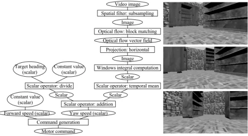
Generally speaking, a vision algorithm can be divided in three main parts: First, the algorithm will process the input image with a number of filters to highlight some features. In our case, this filter chain consists of spatial and temporal filters, optical flow calculation and projection that will produce an image highlighting the desired features. Then these features are extracted, i.e. represented by a small set of scalar values. We implemented this with a mean computation of the pixel values on several windows of the transformed image(s). Finally these values are used for a domain dependent task, here to generate motor commands to avoid obstacles. Fig. 1 shows an example program for a simple obstacle avoidance be-havior based on optical flow. Here is the list of all the primitives (transformation steps) that can be used in the programs and the data types they manipulate:
– Spatial filters (input: image, output: image): Gaussian, Laplacian, thresh-old, Gabor, difference of Gaussians, Sobel and subsampling filter.
– Temporal filters (input: image, output: image): pixel-to-pixel min, max, sum and difference of the last two frames, and recursive mean operator. – Optical flow (input: image, output: vector field ): Horn and Schunck global
regularization method, Lucas and Kanade local least squares calculation and simple block matching method. The rotation movement is first eliminated by a transformation of the two images in order to facilitate further use of the optical flow.
– Projection(input: vector field, output: image): Projection on the horizontal or vertical axis, Euclidean or Manhattan norm computation, and time to contact calculation using the flow divergence.
Fig. 1.Left: Algorithmic tree of a program example for obstacle avoidance. Rectangles represent primitives and ellipses represent data. Right: Snapshots of the simulation environment.
– Windows integral computation (input: image, output: scalar ): For this transformation, we define a global coefficient α0and several windows on the left half of the image with different positions and sizes. With each window is paired a second window defined by symmetry along the vertical axis. A coefficient αi and an operator (+ or −) are defined for each pair. The resulting scalar value R is a simple linear combination calculated with the following formula:
R = α0+Pn i=1αiµi
µi = µLi+ µRi or µi= µLi− µRi
where n is the number of windows and µLi and µRi are the means of the pixel values over respectively the left and right window of pair i.
– Scalar operators(input: scalar(s), output: scalar ): Addition, subtraction, multiplication and division operators, temporal mean calculation and simple if-then-else test.
– Command generation (input: two scalars, output: command ): The mo-tor command is represented by two scalar values: the requested linear and angular speeds.
Most of those primitives use parameters along with the input data to do their calculations (for example, the standard deviation value for the Gaussian filter or the number and position of windows for the windows integral computation). Those parameters are specific to each algorithm; they are randomly generated when the corresponding primitive is created by the evolution process.
2.2 Evaluation in the Simulation Environment
For the evaluation of the different obstacle avoidance algorithms, we use a simu-lation environment in which the robot moves freely during each experiment. The simulation is based on the open-source robot simulator Gazebo. The simulated camera produces 8-bits gray-value images of size 320×160 (representing a field of view of approximately 100◦× 60◦) at a rate of 10 / sec. The simulation environ-ment is a closed room of 36 m2 area (6 m × 6 m) containing three bookshelves (Fig. 1). All the obstacles are immovable to prevent the robot from just pushing them instead of avoiding them. In each experiment, the goal of the robot is to go from a given starting point to a goal location without hitting obstacles.
Due to the complexity of the vision algorithms, we’re limited to about 40,000 evaluations to keep the evolution time acceptable (a few days at most). We therefore face a common problem with genetic programming systems, that is the state space is immense compared to the number of evaluations so large parts of it will never be explored. More, the fitness landscape is very chaotic so the evolution can easily get stuck in a local minima of the fitness function. In previous work we showed that a classical evolution process often produces controllers with a seemingly random trajectory, even if the visual features they use are coherent with the environment [11]. To overcome those problems, we propose a novel approach based on the imitation of a given behavior in a first phase to guide the evolution toward more efficient solutions in the second phase.
2.3 First Phase: Evolution of Algorithms that Imitate a Behavior
In this first phase, the population is initialized with random algorithms and the evolution lasts for 50 generations. The goal will be to match a recorded example behavior. More precisely, we first record the video sequence and parameters of an experiment where we manually guide the robot from the starting point to the target point while avoiding obstacles. We make the trajectory as short and smooth as possible to limit the difficulty of the matching task.
For the evaluation of the algorithms, we replay this sequence and compare the command issued by the evaluated algorithm with the command recorded during the manual control of the robot. The goal is to minimize the difference between these two commands along the recorded sequence. Formally, we try to minimize two variables F and Y defined by the formulas:
F = v u u t n X i=1
(fRi− fAi)2and Y = v u u t n X i=1 (yRi− yAi)2
where fRiand yRiare the recorded forward and yaw speed commands for frame i, fAiand yAiare the forward and yaw speed commands from the tested algorithm for frame i and n is the number of frames in the video sequence.
2.4 Second Phase: Evolution of Efficient Solutions
In this second phase, the population is initialized with the final population of the first phase and the evolution lasts for 50 more generations. The algorithms will be evaluated on their ability to really avoid obstacles and reach the target location. For that, we place the robot at the fixed starting point and let it move in the environment during 30 s driven by the obstacle avoidance algorithm. Two scores are attributed to the algorithm depending on its performance: a goal-reaching score G rewards algorithms goal-reaching or approaching the goal location, whereas contact score C rewards the individuals that didn’t hit obstacles on their way. Those scores are calculated with the following formulas:
G =½ tG if the goal is reached tmax+ dmin/V otherwise C = tC
where tG is the time needed to reach the goal in seconds, tmax is the maximum time in seconds (here 30 s), dmin is the minimum distance to the goal achieved in meters, V is a constant of 0.1 m/s and tC is the time spent near an obstacle (i.e. less than 18 cm, which forces the robot to keep some distance away from obstacles). The goal is hence to minimize those two scores G and C.
For the two phases of evolution, the evaluations consist in fact in two runs with a different starting point and a different goal location. Final scores are the sum of the scores obtained for the two runs. Performing two different runs favors algorithms with a real obstacle avoidance strategy while not increasing evaluation time too much. The starting points are fixed because we want to evaluate all algorithms on the same problem.
2.5 The Genetic Programming system
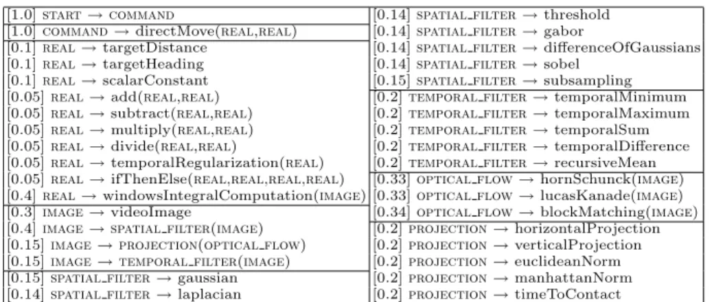
We use grammar based genetic programming to evolve the vision algorithms [12]. As usual with artificial evolution, the population is initially filled with randomly generated individuals. In the same way that a grammar can be used to generate syntactically correct random sentences, a genetic programming grammar is used to generate valid algorithms. The grammar defines the primitives, data and the rules that describe how to combine them. The generation process consists in successively transforming each non-terminal node of the tree with one of the rules. This grammar is used for the initial generation of the algorithms and for the transformation operators. The crossover consists in swapping two subtrees issuing from identical non-terminal nodes in two different individuals. The mutation consists in replacing a subtree by a newly generated one. Table 1 presents the exhaustive grammar that we used in all our experiments.
The numbers in brackets are the probability of selection for each rule. A major advantage of this system is that we can bias the search toward the usage of more promising primitives by setting a high probability for the rules that generate them. We can also control the size of the tree by setting small probabilities
[1.0] start → command [0.14] spatial filter → threshold [1.0] command → directMove(real,real) [0.14] spatial filter → gabor
[0.1] real → targetDistance [0.14] spatial filter → differenceOfGaussians [0.1] real → targetHeading [0.14] spatial filter → sobel
[0.1] real → scalarConstant [0.15] spatial filter → subsampling [0.05] real → add(real,real) [0.2] temporal filter → temporalMinimum [0.05] real → subtract(real,real) [0.2] temporal filter → temporalMaximum [0.05] real → multiply(real,real) [0.2] temporal filter → temporalSum [0.05] real → divide(real,real) [0.2] temporal filter → temporalDifference [0.05] real → temporalRegularization(real) [0.2] temporal filter → recursiveMean [0.05] real → ifThenElse(real,real,real,real) [0.33] optical flow → hornSchunck(image) [0.4] real → windowsIntegralComputation(image) [0.33] optical flow → lucasKanade(image) [0.3] image → videoImage [0.34] optical flow → blockMatching(image) [0.4] image → spatial filter(image) [0.2] projection → horizontalProjection [0.15] image → projection(optical flow) [0.2] projection → verticalProjection [0.15] image → temporal filter(image) [0.2] projection → euclideanNorm [0.15] spatial filter → gaussian [0.2] projection → manhattanNorm [0.14] spatial filter → laplacian [0.2] projection → timeToContact
Table 1.Grammar used in the genetic programming system for the generation of the algorithms.
for the rules that are likely to cause an exponential growth (rules like real → ifThenElse(real,real,real,real) for example).
As described previously, we wish to minimize two criteria (F and Y in the first phase, G and C in the second phase). There are different ways to use evolutionary algorithms to perform optimization on several and sometimes conflicting criteria. For the experiments described in this paper, we chose the widely used multi-objective evolutionary algorithm called NSGA-II. It is an elitist algorithm based on the non-dominance principle. A diversity metric called “crowding distance” is used to promote diversity among the evolved individuals. All the details of the implementation can be found in the paper by K. Deb [13].
In order to prevent problems of premature convergence, we separate the population of algorithms in 4 islands, each containing 100 individuals. Those islands are connected with a ring topology; every 10 generations, 5 individuals selected with binary tournament will migrate to the neighbor island while 5 other individuals are received from the other neighbor island. For the parameters of the evolution, we use a crossover rate of 0.8 and a probability of mutation of 0.01 for each non-terminal node. We use a classical binary tournament selection in all our experiments. Those parameters were determined empirically with a few tests using different values. Because of the length of the experiments, we didn’t proceed to a thorough statistical analysis of the influence of those parameters.
3
Experiments and Results
3.1 Comparison with Other Evolution Strategies
We compare here our own system with a classical one-phase evolution process and with two methods commonly used to guide the evolution toward promising solutions, namely incremental evolution and seeding. For these three experiments
we only use the evaluation function described in 2.4, to select the controllers on their ability to reach the goal while avoiding obstacles.
Seeding an evolution consists in inserting in the initial population one or several individuals (generally hand written solutions) performing reasonably well on the target problem. This seeding method guides the evolution towards a specific part of the state space where we know that there is a good probability to find interesting solutions. Here we simply inserted our manually designed controller presented before in the initial population of one of the four islands. The evolution then proceeds normally for 100 generations.
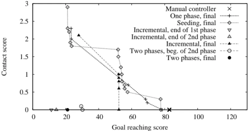
Incremental evolution [14] is based on the decomposition of a problem in a set of problems of increasing complexity. Starting with a simple problem, the evolution quickly finds good solutions. The difficulty is then progressively in-creased and new individuals emerge to adapt to those more and more complex conditions. Here, we proceed for the 20 first generations with a simplified envi-ronment with only one bookshelf (the one that is closest to the wall). This way, there is no real obstacle between the starting points and the target points. Then we proceed for 40 more generations with one more bookshelf, and finally for the 40 last generations with the complete environment containing three bookshelves. In total, all the experiments last for 100 generations, that is 40,000 evalua-tions. Fig. 2 presents the Pareto fronts at different times of the evolution for the different methods. With the classical one-phase evolution, the first generation contains only individuals with poor performance. After 50 generations we obtain controllers with interesting behaviors, performing better than the hand designed controller. The end of the evolution doesn’t improve these results much, we can say here that the evolution process has become stuck in a local minimum of the fitness function. With seeding, the first generations contain better controllers due to the seed individual but the evolution doesn’t manage to further improve this behavior. In the incremental evolution experiment, the evolution finds very efficient controllers in the two first environments. But when we introduce the third bookshelf, the evolution doesn’t find a way to adapt to those new con-ditions. Nevertheless the final controllers perform better than in the previous cases. With two-phase evolution, we obtain very good individuals even at the end of the first phase. The second phase will then optimize those controllers and the final ones definitely surpass the ones obtained with the other methods.
3.2 Analysis of the Controllers
We represent on Fig. 3 the trajectories of the robot in the environment with controllers issued from the different evolution processes. The hand written con-troller manages to avoid obstacles but the robot goes too slowly and never reaches the target points. With the one-phase evolution process, the evolved controllers sometimes manage to reach one of the target points without hitting obstacles but generally they move in an almost random way and with a lot of rotations. Turning quickly on themselves prevents the robots from getting stuck against obstacles and thus generally improves their goal reaching score in the first gen-erations. This kind of controllers quickly overcomes the rest of the population
0 0.5 1 1.5 2 2.5 3 0 20 40 60 80 100 120 Contact score
Goal reaching score
Manual controller One phase, final Seeding, final Incremental, end of 1st phase Incremental, end of 2nd phase Incremental, final Two phases, beg. of 2nd phase Two phases, final
Fig. 2.Pareto fronts at different times of evolution for the different evolution strategies. Those fronts are created by taking the best individuals in the generation in all the four islands and keeping only non-dominated ones. In some cases one individual dominates all others, reducing the front to one point.
and prevents the evolution from finding better controllers. As shown before, the seeded evolution didn’t manage to improve the seed individual much. The tra-jectory obtained with evolved controllers is very close to the tratra-jectory of the hand written controller used as seed.
The incremental evolution produces efficient solutions with one and two book-shelves but when we add the final one, the evolution fails to adapt the controllers. The trajectory clearly shows this problem: one of the bookshelf is quickly avoided but the robot just stops before hitting the second one without trying to avoid it. The first phase here selects very simple controllers going straight on to the target points. To achieve this, they just use the target heading value for the yaw speed command. Although it is a good strategy without obstacles, these controllers are difficult to adapt afterward for more complex problems.
With two-phase evolution, the first phase evolves controllers with smooth trajectories very similar to the recorded sequence. Some of those controllers even reach the two target points although most of them get stuck on an obstacle as shown on Fig. 3. With this initialization, the second phase quickly evolves very efficient controllers reaching the two target points without hitting obstacles and even faster than when the robot is manually controlled. The structure of the controllers evolved in this environment is generally quite simple (mainly based on contrast information obtained with simple threshold filters) and there’s almost no structure difference between the end of the first phase and the end of the second phase. This means that the imitation phase is crucial for the evolution of the structure to produce efficient controllers. The second phase mainly optimizes the parameters of the algorithms to obtain a faster and more robust behavior.
The main limitation of all those controllers is that they don’t generalize well to different conditions. If we move around the obstacles, the starting point
a b c d e f g Starting point 1 Target point 1 Trajectory 1 Starting point 2 Target point 2 Trajectory 2 Contact points
Fig. 3. a) Trajectory of the hand written controller. b) Trajectory of a controller evolved with one-phase evolution. c) Trajectory of a controller evolved with seeded evolution. d) Trajectory of a controller evolved with incremental evolution. e) Trajec-tory of the recorded sequence. f) TrajecTrajec-tory of a controller evolved with only example matching evaluation during 50 generations (end of the first phase). g) Trajectory of the controller evolved with two-phases evolution process (end of the second phase). The small dots on the trajectories are placed every 2 seconds and thus indicate the speed of the robot.
and the target point, the performance of the controllers decreases quickly. The controller issued from two-phase evolution still shows some obstacle avoidance abilities but it doesn’t move toward the target point. Some other controllers just seem to move randomly in the environment. There are two reasons for this mediocre generalization behavior: First, it seems that the choice of only two trajectories in the evaluation environment was too optimistic. The controllers overlearn these trajectories and this decreases their generalization performance. Second, the evolved controllers often use the target heading information in quite complicated ways or even not at all. In this case when we move the target point they are not able to find it unless by chance. To overcome these problems we have designed experiments with more trajectories during the evolution and with a different grammar which facilitates an efficient use of the target heading for the controllers. The generalization performance of the controllers evolved this way is presented in [15].
4
Conclusion
In this paper, we present a system that selects and adapts automatically an appropriate obstacle avoidance method to a given visual context. This system is based on genetic programming and we introduced a novel evolution process to guide the evolution toward promising solutions in the state space. We have shown that for our target application, it improves the performance of the final controllers greatly compared to classical evolution, seeding or incremental
evolu-tion. This method could be adapted for many evolutionary robotic systems and it would be interesting to validate it on other applications.
Our goal is now to test this method on a wide range of environments (includ-ing real-world environments) to check if some primitives are selected more often than others and how they are combined by the evolution. This will lead to a bet-ter understanding on how to combine different vision information in a robotic navigation system in order to obtain more adaptive and robust behaviors.
References
1. Muratet, L., Doncieux, S., Bri`ere, Y., Meyer, J.A.: A contribution to vision-based autonomous helicopter flight in urban environments. Robotics and Autonomous Systems 50(4) (2005) 195–209
2. Zufferey, J., Floreano, D.: Fly-Inspired Visual Steering of an Ultralight Indoor Aircraft. IEEE Transactions on Robotics 22(1) (2006) 137–146
3. Malik, J., Perona, P.: Preattentive texture discrimination with early vision mech-anisms. Journal of the Optical Society of America A: Optics and Image Science, and Vision 7(5) (1990) 923–932
4. Michels, J., Saxena, A., Ng, A.: High speed obstacle avoidance using monocular vision and reinforcement learning. Proceedings of the 22nd international conference on Machine learning (2005) 593–600
5. Ulrich, I., Nourbakhsh, I.: Appearance-based obstacle detection with monocular color vision. Proceedings of AAAI Conference (2000) 866–871
6. Walker, J., Garrett, S., Wilson, M.: Evolving controllers for real robots: A survey of the literature. Adaptive Behavior 11(3) (2003) 179–203
7. Marocco, D., Floreano, D.: Active vision and feature selection in evolutionary behavioral systems. From Animals to Animats 7 (2002) 247–255
8. Trujillo, L., Olague, G.: Synthesis of interest point detectors through genetic pro-gramming. Proceedings of the 8th annual conference on Genetic and evolutionary computation (2006) 887–894
9. Pauplin, O., Louchet, J., Lutton, E., De La Fortelle, A.: Evolutionary Optimisation for Obstacle Detection and Avoidance in Mobile Robotics. Journal of Advanced Computational Intelligence and Intelligent Informatics 9(6) (2005) 622–629 10. Martin, M.: Evolving visual sonar: Depth from monocular images. Pattern
Recog-nition Letters 27(11) (2006) 1174–1180
11. Barate, R., Manzanera, A.: Automatic Design of Vision-based Obstacle Avoidance Controllers using Genetic Programming. Proceedings of the 8th International Con-ference on Artificial Evolution, EA 2007, LNCS 4926 (2008) 25–36
12. Whigham, P.: Grammatically-based genetic programming. Proceedings of the Workshop on Genetic Programming: From Theory to Real-World Applications (1995) 33–41
13. Deb, K., Pratap, A., Agarwal, S., Meyarivan, T.: A fast and elitist multiobjective genetic algorithm: NSGA-II. IEEE Transactions on Evolutionary Computation 6(2) (2002) 182–197
14. Gomez, F., Miikkulainen, R.: Incremental Evolution of Complex General Behavior. Adaptive Behavior 5(3-4) (1997) 317–342
15. Barate, R., Manzanera, A.: Generalization Performance of Vision Based Con-trollers for Mobile Robots Evolved with Genetic Programming. Proceedings of the Genetic and Evolutionary Computation Conference (2008) To Appear