Psychological trade

Psychological Trade

M. Blanchard and F. Peltrault

EURIsCO, INALCO and EURIsCO, University Paris Dauphine Place du Maréchal de Lattre de Tassigny 75775 Paris cedex 16

Abstract

Section 1. Introduction

As reported by the Global Entrepreneurship Monitor [2002], 10.51% of the adult population is involved in the creation and growth of start up businesses in the United States. The rate of entrepreneurial activity is lower in the main trade partners of the United States: 1.81% in Japan, 3.2% in France, 5.16% in Germany and 5.37% in the United Kingdom. According to European Commission, Europe suffers from an entrepreneurship deficit in comparison to the US which could damage the long term growth of European countries. The purpose of this paper is to challenge the link between entrepreneurship and international trade and the resulting welfare consequences. How to characterize psychological differences between managers and countries? Should European countries avoid risk and let the United States undertake risky innovative activities? Can free trade rectify the consequences of entrepreneurship deficit on countries’ welfare?

According to De Meza and Southey [1996], an entrepreneur is a manager who overestimates his chance of success1. Because entrepreneurs are optimistic, they will undertake new innovative activities. This definition recalls Schumpeter’s essentialist view of the entrepreneur according to which some (superior) people are born entrepreneurs and some are

not. In this paper, we adopt the behavioural definition of Kihlstrom and Laffont [1979] for whom a manager becomes an entrepreneur because he has chosen the risky activity rather than the certain activity.

Entrepreneurs can deal with both global and idiosyncratic risks. The consequences of global uncertainty on international trade have already been studied2 since the pioneering work of Brainard and Cooper [1968]. Mayer [1976] and Sakai [1978] examine the consequences of price uncertainty. Helpman and Razin [1978] study the consequences of global technological uncertainty on the positive theorems of international trade. Newbery and Stiglitz [1984] and Shy [1988] relax the assumption of perfect correlation between the uncertainty in a given sector in each country. They show that free trade can lower the ex-ante welfare when global risk is negatively correlated between countries.

We depart from these frameworks by introducing idiosyncratic risk without insurance market. As documented by Moskovitz and Vissing-Jorgensen (2002), idiosyncratic risk is a key feature of entrepreneurial investment leading to a great dispersion in return of private equity. They also point out that entrepreneurial investment is very concentrated. This lack of diversification is very puzzling because the return of entrepreneurship tends to be low when controlling for risk.

In order to cope with both optimism and pessimism, we assume that managers misperceive their objective probability of success. This behaviour is well known since Kahneman and Tversky [1979]. In addition, Cooper, Woo and Dunkerberg [1988] reveal a great diversity of attitude towards risk among entrepreneurs in the United States. Some entrepreneurs are pessimistic e.g. 1% of them see a probability of success of 0.1 while some are optimistic e.g. 33% see a probability of success of 1. But the population of entrepreneurs surveyed in the United States seems rather optimistic. In fact, 81% of entrepreneurs see a probability of success more than 0.7 whereas numerous studies suggest that less than 50% of businesses survive for more than five years. Though there exist both optimistic and pessimistic managers in each country, Hofstede [2001] emphasizes that countries are heterogeneous regarding their uncertainty avoidance. For example, the level of uncertainty avoidance is twice as much in Japan than in the United States.

In this model, trade is grounded on cross-country differences in managers’ attitude towards risk. The relatively more optimistic country exports the risky commodity while the other country exports the certain commodity. The welfare analysis is more complicated since there is a need for both ex-ante and ex-post analysis according to Hammond [1981]. On the one hand, the ex-ante welfare analysis is useful to understand why managers will lobby in favour

or against free trade commitment. On the other hand, this decision made prior to the resolution of uncertainty can be regretted if the ex-post welfare analysis based on effective consumption leads to an opposite statement.

Numerical simulations show that free trade is not always welfare improving. Ex- ante and

ex-post welfare may decrease with the opening of trade. Moreover decisions are made before the

resolution of uncertainty that can be later regretted. In addition, the world as a whole can be worse off after trade when we look at effective consumption. Therefore, lump-sum transfers are not always sufficient to compensate trade losses.

The paper is organized as follows. Section 2 describes the structure of the model. Section 3 analyses the autarky equilibrium. Section 4 examines the free trade equilibrium and ex ante and ex post welfare effects. Section 5 gives economic interpretations and Section 6 studies economic policy implications. Section 7 concludes.

Section 2. The model

Consider a country J in which a continuum of managers indexed on the interval

[

0;1

]

have to choose exclusively between two production project C and R. It is assumed that managers are totally involved in the management of their production project. In fact, Moskowitz and Vissing-Jørgensen [2002] document that entrepreneurs and private investors face a dramatic lack of diversification and an extreme dispersion in returns. Project C is certain and provides one unit of commodity C and the wage w . Project R is risky since it provides one unit of commodity _c R and the wage w_r with probability θ and 0 with probability 1-θ. Hence, risk is idiosyncratic to each manager’s project rather than global because aggregate uncertainty is cancelled by application of the law of large numbers. As quoted by Judd [1985], there are some difficulties with the application of the law of large numbers in a continuum. However, we follow here the tradition of economic literature3 which explicitly or implicitly avoids this difficulty.

2.1 Psychology of managers

Despite the probability of success θ is common knowledge, we assume each manager

[ ]

0;1

i∈ have their own perceived probability of success denoted by g_θ(i). Cooper, Woo & Dunkerberg [1988] show that “the assessment by entrepreneurs of their own likelihood of success is dramatically detached from past macro statistics, from perceived prospects for peer businesses, and from characteristics typically associated with higher performing new firms.”

Moreover, this behaviour tends to persist because people are reluctant to reconsider their self-image. Then it seems reasonable to assume that managers will resist to Bayesian revisions in order to maintain their self-confidence4.

Consider that managers are ranked in the continuum

[ ]

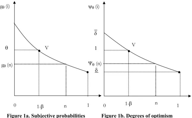
0;1 according to their subjective probability and their degree of optimism δ which can be defined as follows:

θ = Ψ = δ_{θ θ}(i) gθ(i) with     θ ∈

δ_θ 0;1 . A manager i becomes optimistic if Ψ_θ(i)>1. Let for commodity of notation δ_θ =δ.

Figures 1a and 1b give an illustration of the distribution function of managers regarding their perceived probability of success and their degree of optimism.

Figure 1a. Subjective probabilities Figure 1b. Degrees of optimism

Consider two managers j and k. Then, the manager j is relatively more optimistic than manager k if and only if j< : k

k j ) k ( g ) j ( g_θ > _θ ⇔ < and Ψ_θ(j)>Ψ_θ(k)⇔ j<k

δ (resp. δ) refers the degree of optimism of the more optimistic manager (less optimistic):

) 0 ( θ Ψ = δ and δ=Ψ_θ(1). Example

4 _{Benabou and Tirole [2002] assume an imperfect Bayesian revision grounded on a psychological literature} (Ross and Anderson [1977] among others).

0 1 1 ψθ (i) 1-β 0 1 θ gθ (i) δ δ 1-β V V n n gθ (n) Ψθ (n)

Define the distribution function of subjective probabilities as g_θ(i)=θβ+i with _ _ θ ∈

β 0;1 . Then, the population of managers can be break down into two groups: optimistic managers and pessimistic ones managers.

– managers are optimistic whateverj∈

[

0;1−β

[

,g_θ(j)>θ andΨ_θ(j)>1 – managers are pessimistic whateverj∈

]

1−β;1

]

,g_θ(j)<θ andΨ_θ(j)<1 – Manager V indexed by1−β is realist since g_θ(1−β)=θ andΨ_θ(1−β)=1 2.2 Decision rule

Managers have to choose before the resolution of uncertainty. The dual theory of choice under risk introduced by Yaari [1987] is useful to deal with how the perceived risk of managers is processed into the production choice. This is the case because the utility function defined by Yaari [1987] is linear in income. Consider gamble L with two outcomes. The value of the outcomes is ( x ,x) with associated objective probabilities (θ,1−θ).

Following Yaari, the utility function of a manager i becomes:

x ) ( g x )] ( g 1 [ ) L ( _{i i} i = − θ + θ Ω ,

where g_i(θ)denotes the function of perceived probabilities by a manager i. Note that g_i(θ) is monotonously increasing in θ with gi(0) = 0 and gi(1) = 1. Then a manager is optimistic (pessimistic) when g_i(θ) is concave (convex).

In this model, each manager has to choose between a certain project and a risky project which provides the wage w_r with probability θ and 0 with probability 1-θ. Regarding the subjective probability g_i(θ) of manager i, his prospect of the risky project R is:

r i

i

i(R)=[1−g (θ)]×0+g (θ)×w

Ω .

Then, we have the following decision rule for each manager i∈

[ ]

0;1 .

Decision rule: A manager i chooses to product risky commodity if and only if:

c r i i i(R)>Ω (C)⇔g (θ)×w >w Ω (1)

The level of entrepreneurship in the economy depends on the distribution function of subjective probability but also on the equilibrium wage.

Section 3. Autarky.

The level entrepreneurship of country J in autarky is given by n that is the share of a_J managers involved in the risky project. In fact, the manager indexed by n is indifferent a between project R and project C. For this critical manager, we have

RJ CJ a J J a J a RJ a J a CJ _w w ) n ( and w ) n ( g w θ = Ψ = δ × =

The degree of optimism associated with this manager is equal to the objective relative wage. The level of entrepreneurship in autarky is clearly equal to n since more optimistic a managers than the critical manager will choose the risky project:

[ ]

0;n , (i) and (R) (C) i∈ a Ψ_J ≥δa Γ_i >Γ_i

∀ .

Production of commodity R in autarky is thenya_RJ =θna_RJ 3.2. Relative price and wage in autarky

Commodity C is the numéraire so p refers to the autarky price of commodity R in terms of a_J commodity C. After the resolution of uncertainty, managers involved in the certain activity receive wa_CJ =1 while lucky entrepreneurs earn wa_RJ =pa_J. The relative wage in autarky is given by wa_CJ wa_RJ =1 pa_J .

Income is consumed after the resolution of uncertainty. Let d_CJ and d_RJ be the demand for commodity C and R respectively. Aggregate demand functions for the two commodities have unitary price and income elasticities and b denotes the share of income devoted to the consumption of commodity R. We haved_CJ =(1−b)y_J and d_RJ =by_J p where y is the _J aggregate income of country J with ya_J =(1−na_J)+p_Jaθna_J.

Then, the relative price of commodity R which equals demand and supply of commodity R is given by a J a J a J n n 1 ) b 1 ( b p × − θ × −

= . It depends on the objective probability θ, on the share of entrepreneurs and on demand conditions.

3.3. Autarky equilibrium.

General autarky equilibrium is reached when the risky commodity market clears. At the equilibrium price, the amount of risky commodity demanded by all agents equals the amount supplied (ex post) by managers who have chosen (ex ante) the risky process. Formally, as in Kihlstrom and Laffont (1979), an equilibrium is a partition

{ }

∆,Γ of the continuum

[ ]

0,1 and a price p, that is a pair

(

{ }

∆,Γ,p

)

; for which global supply is equal to global demand of the risky commodity. Let n the number of managers who are members of ∆ . We call them the a_J

entrepreneurs as they will undertake the risky project. Let 1−na_J the number of managers who are members of Γ .

Since decision is made before the resolution of uncertainty, managers have to anticipate the level of earnings provided by each production project. This is possible as long as the distribution function of managers regarding their subjective probability is common knowledge. The psychological structure of the country is needed to anticipate the level of entrepreneurship and the equilibrium price of the risky commodity.

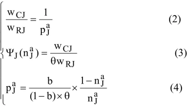
Then the following equations identify the autarky equilibrium in country J:

           − × θ × − = θ = Ψ = (4) n n 1 ) b 1 ( b p (3) w w ) n ( (2) p 1 w w a J a J a J RJ CJ a J J a J RJ CJ

Equation (2) gives the relative wage after resolution of uncertainty. Equation (3) states that managers are indifferent between C and R if the expected wages delivered by each project are equal. The relative price of commodity R which equals global demand and global supply of commodity R is given by equation (4).

Then, the level of entrepreneurship in autarky is given Ψ_J(na_J)=φ(na_J) where

a J a J a J n n 1 ) b 1 ( b ) n ( × − θ × − = φ .

Proof of the existence and the uniqueness of the equilibrium level of entrepreneurship are given in appendix A, but a diagram can help to illustrate the properties of the autarky equilibrium.

3.4. Diagrammatic exposition

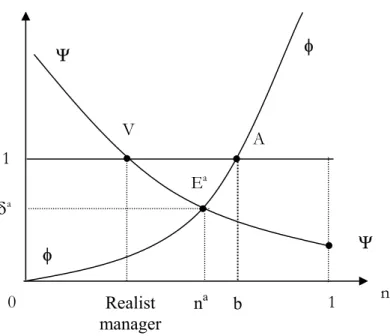
Figure 2 shows how the functions Ψ_J(na_J) and φ(na_J) determine the equilibrium allocation of managers in industry R.

Figure 2. Autarky equilibrium

The autarky level of entrepreneurship n (i.e the ranking of the critical manager) is at point a_J

a

E where ΨΨ and φφ intersect. When all managers are realist like manager V, the equilibrium level of entrepreneurship is equal to the share of the national income devoted to consumption of risky commodity : na_J = . This benchmark helps to characterize the overall b psychology of a country.

Definition 1. A country J will be J globally optimistic if the critical manager is optimistic the equilibrium level (δa_J >1). Saying differently, a country will be optimistic if the equilibrium level of entrepreneurship is higher than b. Otherwise country J will be pessimistic.

Figure 2 shows the case for a globally pessimistic economy since the production of risky commodity is inferior to b. The decision of realist manager

(

δ=1

)

reveals the attitude towards risk of the country. Here, he chooses the risky project as the remuneration of the risky commodity is higher than the relative expected productivities:. Since the economy is globally pessimistic a positive risk premium (pa −1 θ>0) is needed to incite managers to undertake the risky project. On the contrary, risk premium will be negative (pa −1θ<0) in optimistic countries.

Section 4. International Trade

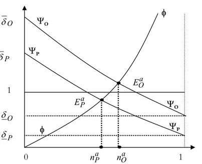
Consider two countries O and P. Those countries differ only according to the psychological structure of managers. Country O is relatively more optimistic than country P:

] [

0;1 , (n) (n) n∈ Ψ_O >Ψ_P ∀ φ V Ea 1 Realist manager 0 φ na Ψ 1 n δa A b Ψ

A given entrepreneur n of country O is always more optimistic than the same entrepreneur n in P. For a given degree of optimism δ, the share of entrepreneurs is higher in O than in P. 4.1. The law of comparative advantages.

The law of comparative advantages holds and the differences in autarky prices determine the structure of international trade. In the state of autarky, the relative price in country j = O; P is written: a j a j 1 p θδ = then pa_O <pa_P ⇔δ_Oa >δ_Pa.

As demand conditions are identical in two countries, comparative advantages only depend on international differences in the psychological structure of managers.

Proposition 1 : Country O has a comparative advantage in the production of the risky commodity as the critical manager is, in autarky, relatively more optimistic in country O than in country P.

Figure 3. Comparative advantages

Figure 3 illustrates proposition 1 with β_O <β_P. Country O has more entrepreneurs in autarky than country P. Relative price of risky commodity is cheaper in O than in P before trade. 4.2. Free Trade Equilibrium

Under free trade, each manager knows the psychological structure of the two countries. Then, a manager can deduct the free trade international price of risky commodity and then he

E _Pa δ_P φ n _Oa n _Pa E _Oa δP δO 1 0 1 Ψ_O δ_O Ψ_P Ψ_P Ψ_O φ

chooses. The free trade equilibrium price is deducted from the clearing of the aggregate demands and the aggregate supplies of the world:

(

+

)

θ = *_O *_P *_{r n n} y and

(

)

* *_P * O *_r p y y b d = × + with y_j* ₌p*_θn*_{j +}

(

1₋n*_j

)

j₌O,P. Then the free trade equilibrium gives

. n n n 1 n 1 ) b 1 ( b p *_P * O *_P * O * + − + − × θ − =

As in autarky, the degree of optimism of indifferent (critical) managers _{δ is determined.} *

*_P *_O *_P *_O * n 1 n 1 n n b b 1 − + − + × − = δ

Free trade equilibrium exists and is unique (proof: see Appendix B). In each country, relatively optimistic managers, i.e those who have a degree of optimism higher than _{δ ,} *

product the risky commodity. By definition, for a given degree of optimism δ, the share of entrepreneurs is higher in O than in P. International trade will occur.

Proposition 2 Under free trade, the relative price of the risky commodity is between the relative autarky prices: a * a_P

O p p

p ≤ ≤ . When demand conditions are identical, the relatively more optimistic country will specialize in the production of the risky commodity while the relatively pessimistic country will specialize in the production of the certain commodity. Proof is given in appendix C.

Section 5. Welfare Analysis

5.1. The need for both ex ante and ex post welfare analysis.

As quoted by Hammond [1981, p.238], “Ex ante efficiency loses some of its normative appeal when consumers misperceive probabilities, or when they have inappropriate attitudes towards risk, or even if they are concerned about inequality of income ex post. In such cases, one becomes interested in different concepts of efficiency and of welfare optimality. These are based on a consumer’s welfare ex post. (…) The whole problem of uncertainty is that decisions are made that are latter regretted.” Hence, it is necessary to build the welfare impact of trade liberalization both on ex ante and ex post criterions as managers misperceive probabilities.

Ex post analysis evaluates the level of aggregate utility after the resolution of uncertainty. It compares utility resulting from effective consumption under autarky and free trade. So, it is

not a psychological but a concrete criterion as it is grounded on what managers will effectively consume.

5.2. Ex ante welfare analysis. 5.2.1. Methodology

The ex ante analysis compares the economy in a state of autarky under autarky to an economy in a state of free trade before the resolution of uncertainty. Ex ante welfare depends on the expected income of managers given their perception of risk.

Regarding the demand functions depicted in section 3, the underlying expected utility function of a given manager i before the resolution of uncertainty is :

( )

_ik b b 1 b ik b (1 b) E y~ p U = − − − with k=R ,C

where E

( )

y~_i is the expected income of manager i which depends on the production choice:

( )

   = θ = = R k for p ) ( g C k for 1 y~ E i ik

Hence the expected utility of managers is

    = θ − = − = − − − − R k for p ) ( g ) b 1 ( b C k for p ) b 1 ( b V b 1 i b 1 b b b 1 b ik

The ex ante welfare of an entrepreneur is related to his psychology. Since each entrepreneur

has his own perception of probabilities, each manager has his own ex ante evaluation. Then,

an aggregation problem arises and the Hicksian compensation measure of welfare is used to cope with this difficulty. This measure gives, for each manager, the lump-sums transfer required to maintain under free trade the same level of utility as in autarky. Denote Ti the measure of Hicksian compensation which leaves unchanged the expected utility level of manager i. Hence, Ti is such that :

[

E

( )

y~_ik +T_i

]

p*−b =E

( )

y~_ik pa−b.

Then, country J is better off when the sum of the compensated incomes is negative:

0 di T T 1 0 i J =

∫

< .

5.2.1.1. The case of the pessimistic country

Recall that the level of entrepreneurship is given by the critical manager denoted by na in autarky and n* under free trade. It is necessary to calculate the compensated income of three types of managers.

For this partition of the continuum, the compensated income Ti is given by

( )

[

]

( )

[

( )

]

_{* b}

[

_a

( )

]

_a b i * b a ik b * i ik T p E y~ p p g i T p p g i p y~ E + − = − ⇔ _θ + − = _θ − . So we have T_i g

( )

i p*b pa1 b p*1 b_>0      ₋ = _θ − −

These managers are worse off with trade since the relative price of commodity R is decreasing with the opening of trade from the pessimistic country’s point of view.

Type 2. Managers i_∈

[

max

(

n*,na

)

;1

]

_{still produce commodity C with the opening of trade.} For this partition of the continuum, the compensated income Ti is given by :

( )

[

]

( )

[

]

_{* b a} b i b a ik b * i ik T p E y~ p 1 T p p y~ E + − = − ⇔ + − = − So we have, 1 0 p p T _b a b * i = − < .

These managers are better off with trade due to the decrease of relative price of commodity R. Type 3. Managers i∈

[

n*,na

]

abandon the risky project for the certain one:

( )

[

]

( )

[

]

_{* b}

[

_a

( )

]

_a b i b a ik b * i ik T p E y~ p 1 T p p g i p y~ E + − = − ⇔ + − = _θ − So we have, T_{i =}p*bpa1−bg_θ

( )

i ₋1_.

Hence, the sum of compensated incomes for the pessimistic country is :

( )

( )

1di p p di 1 i g p p di i g p p p di T 1 n ab b * n n b 1 a b * n 0 b 1 * b 1 a b * 1 0 i a a * *

∫

∫

∫

∫

       − +       ₋ +       ₋ = − − _θ − _θ

5.2.1.2. The case of the optimistic country

There are two differences with the pessimistic country. First the boundaries of integrals are different since the level of entrepreneurship increases with the opening of trade (_n* _>na_).

Second, managers changing their production choice abandon the certain commodity for the risky one.

Type 3. Managers i∈

[

na,n*

]

abandon the certain project for the risky one:

( )

[

]

( )

[

( )

]

_{* b a} b i * b a ik b * i ik T p E y~ p p g i T p p y~ E + − = − ⇔ _θ + − = − So we have, p g

( )

i p p T * b b * i = − θ

( )

( )

1di p p di i g p p p di i g p p p di T 1 n ab b * n n * b a b * n 0 b 1 * b 1 a b * 1 0 i * * a a

∫

∫

∫

∫

       − +         − +       ₋ = − − _{θ θ} 5.2.2 Simulation results

There are no analytic solutions as equations are non-linear. Hence numerical simulations of equilibrium and ex ante welfares are implemented with specification of countries’ psychological structure. Simulation 2 shows that the more pessimistic country can be worse off with trade for some values of parameters. On the contrary, the more optimistic country and the world are always better off for all the specifications tested. In particular, the results of two simulations among others are described below.

Simulation 1

The psychological structure of managers is _ΨO(n)=θ0.3−1+n _and n P(n)= 0.3−1+2

Ψ θ .

With b = 0.51 and θ = 0.45, we obtain a =1.13

O

δ , 832a =0.

P

δ and δ* =1.0117. The sum of the compensated incomes are T T di 0.0223

1 0 iO O =

∫

=− ;T T di 0.0052 1 0 iP P =

∫

=− ; that is

country O and P are ex ante better off with trade. Moreover, as

∑

=−

j W 0275 . 0 T , the world is better off. Simulation 2

The psychological structure of managers is n O n = −+

Ψ _{( ) θ}0.3 1 _and n P(n)= 0.3−1+1.4

Ψ θ .

With b = 0.51 and θ = 0.45, we obtain δOa =1.13, δPa =0.99 and δ* =1.069. Compensated

incomes are T_O =−0.0086;T_P =0.0028; that is country O is better off with trade while country P is worse off with trade. Moreover, the world is better off since

∑

=−

j W 0058 . 0 T . Summary

The impact of free trade on ex ante welfare can be summarized in table 1 and in the following proposition.

Proposition 3 When risk is idiosyncratic and managers are heterogeneous regarding their subjective probabilities, international trade may decrease the ex-ante welfare of the more pessimistic country.

5.3.1 The optimum level of entrepreneurship

In autarky, the collective ex post utility of country J is given by:

(

)

_a

( )

_a b J b b 1 a J 1 b b y p V = − − × × × − i.e

(

)

( )

a J b a J b b b 1 a J 1 b b _{1 b b} V δ + − δ × θ × × − = − with

(

)

( )

(

)

(

_a

)

2 J a J 1 a J b b 1 b 2 a J a J b b 1 1 b b 1 d dV δ + − − δ × δ × θ × × − = δ − + −

The collective utility function of country J depends on the psychological structure of the population, on demand conditions and on uncertainty. The first best optimum is reached when the critical manager is realist i.e whenδa_J =1. Then, the level of entrepreneurs is na _{= .} b Hence, we can define entrepreneurship deficit or surplus regarding the optimum level of entrepreneurship.

Definition 2: At the equilibrium, the gap between the effective number of entrepreneurs and the optimum number of entrepreneurs isD₌na ₋b_{. The economy is facing an} entrepreneurship deficit if D < 0 or an entrepreneurship surplus if D > 0.

5.3.2. Simulation results

First, it can be shown (see appendix D) that at least one country is better off with the opening of trade. In fact Country O (P) is always better off if the world economy is globally pessimistic (optimistic). Moreover, a realist country in autarky is always better off with trade. Numerical simulations are needed to draw more conclusions. It appears that the other country and the world can be worse off with trade. The Hicksian compensation method is applied to evaluate the aggregate welfare of the world T . _w

Simulation 1

The Psychological structure of the managers in country O and P are respectively :

n O n = −+

Ψ _{( ) θ}0.3 1 _and n P n = −+

Ψ _{( ) θ}0.7 1

For all simulated values of parameters b and θ the world is always better off (T_w < ). 0 When the world is globally optimistic (_δ* _>1_{), country P is always better off with trade.} Country O can be either worse off or better off with trade depending on the values of parameters.

– with b = 0.35 and θ = 0.45, we have a =1.26

O

δ , 96a =0.

P

δ , 022_δ* ₌1. _{. The impact} of free trade on ex post welfare is ∆V_O =−0.0055 and ∆V_P =0.0072.

– with b = 0.43 and θ = 0.001, we obtain a =2.12

O

δ , 68a =0.

P

δ and _δ* ₌1.2_{. The} impact of free trade on ex post welfare is ∆V_O =0.0002 and ∆V_P =0.0005.

When the world is globally pessimistic (_δ* _<1_{), country O is always better off while country} P can be either worse off or better off according to the values of parameters:

– with b = 0.66 and θ = 0.45, we have a =1.02

O

δ , a =0.78

P

δ and δ* =0.89. The impact of free trade on ex post welfare is ∆V_O =0.0065 and ∆VP =−0.0052.

– with b = 0.51 and θ = 0.45, we obtain a =1.13

O

δ , 87a =0.

P

δ and _δ* ₌0.99_{. The impact} of free trade on ex post welfare is ∆V_O =0.00115 and ∆V_P =0.00035.

Simulation 2

The Psychological structure of the managers in country O and P are respectively:

n O n = −+

Ψ _{( ) θ}0.5 1 _{and ( )} 0.5 1 n0.1

P n = −+

Ψ θ

For some values of parameters, the world is globally pessimistic and is worse off with trade. With b = 0.66 and θ = 0.45 we obtain a =0.89

O

δ , 67a =0.

P

δ and _δ* ₌0.73_{. The} impact of free trade on ex post welfare is ∆V_O =0.0239, ∆V_P =−0.0257 and T_w =0.0071 Note that the aggregate level of entrepreneurs is decreasing: + a =1.22> _O* + *_P =1.18

P a

O n n n

n .

Simulation 3

The Psychological structure of the managers in country O and P are respectively:

n 1 3 . 0 O(n)=θ − + Ψ and Ψ_P(n)=θ0.3−1+3n

For some values of parameters, the world is globally optimistic and is worse off with trade. With b = 0.2 and θ = 0.45 we obtain a =1.42

O

δ , a =1.06

P

δ and δ* =1.3. The impact of free trade on ex post welfare is ∆V_O =−0.0132, ∆VP =0.0127 and Tw =0.001. The

aggregate level of entrepreneurs is increasing: nOa +nPa =0.4711<n*O +nP* =0.4915.

Hence free trade can amplify the autarky distortions: when the world is globally optimistic (resp. pessimistic), it is nevertheless possible that the level of entrepreneurship increases (decreases) with trade..

Summary

The impact of free trade on ex post welfare can be summarized in table 1 and in the following proposition.

Country O Country P World

Optimistic world Better off / worse off Better off Better off / worse off Pessimistic world Better off Better off / worse off Better off/ worse off

Proposition 4 When risk is idiosyncratic, mutual gain from international trade doesn’t always exist. The impact of the opening of trade on the ex post welfare can be either positive or negative depending on the values of parameters. However, when the world is globally pessimistic (optimistic) the welfare of the more optimistic (pessimistic) country increases. Nevertheless, gains from trade of one country not necessarily outweigh losses from trade of the other: world economy can be worse off with trade.

Section 6. Economic Interpretations and policy implications. 6.1. Economic interpretations

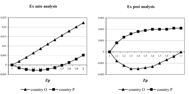
Consider the case of a globally optimistic world. As seen before, free trade always increases the ex-post welfare of country P. This is the case illustrated by figure 4 for some values of

parameters: the ex-post gains from trade of country P are always positive. Country O can be better or worse off depending on the degree of optimism of country P. When the psychological distance with country P is low (Zp<2), country O is worse off. When the psychological distance becomes high enough (Zp>2), country O becomes better off with free trade.

The ex-post welfare of country O is decreasing after trade mainly because the relative price of commodity R is not high enough to reward the risk taken by entrepreneurs. In this globally optimistic world, _{p is lower than the equilibrium price with perfect insurance market}* 5_.

Therefore, the entrepreneurs receive a negative risk premium RP₌p*₋1_θ<0_{. With the} opening of trade, these negative risk premiums flow in country O since the level of entrepreneurship is increasing6. Of course, the risk premium is increasing in comparison to autarky. But, when the psychological distance is low, a slight increase of the risk premium is consistent with a great increase of the level of entrepreneurship in country O.

The world can be worse off with trade too. This is the case of simulation 3 where both countries suffer from entrepreneurship surplus in autarky (δa_o and δ are higher than 1). a_P Here, free trade increases the entrepreneurship surplus at the world level: that is

5 _{With a perfect insurance market, the equilibrium price of commodity R is equal to the ratio of expected} productivities, that is p=1θ.

a P a O * P * O n n n

n + > + . In fact, international trade can amplify the autarky distortions because the relative price of commodity R is not a signal of objective relative productivities but of biased productivities.

Figure 4. The psychological distance between countries and the gains from trade

Ex ante analysis -0,005 0 0,005 0,01 0,015 0,02 0,025 1 1,1 1,2 1,3 1,4 1,5 1,6 1,7 1,8 1,9 2 Zp country O country P Ex post analysis -0,002 -0,001 0 0,001 0,002 0,003 1 1,1 1,2 1,3 1,4 1,5 1,6 1,7 1,8 1,9 2 Zp country O country P

Note : Along the y-axis, ex-ante and ex-post gains from trade are given for both countries. Along the x-axis, Zp is a parameter which influences the degree of optimism of country P: a higher Zp means that country P becomes more pessimistic and that the psychological distance with country O increases. The distribution functions are

n 1 3 . 0 O(n)=θ −+

Ψ and _ΨP(n)=θ0.3−1+Zp×n _{with θ=0,45 and demand conditions are given by b=0,51.}

The ex-ante analysis can provide opposite conclusions as illustrated by figure 4. Contrary to the ex-post analysis, country O is now better off whereas country P is worse off. This is because the risk premium is now subjective and always positive for all the entrepreneurs. Before the resolution of uncertainty, the subjective risk premium is given by p* ₋1 g_i(_θ) which is positive for all _i∈

[ ]

_0,n* _{. With the opening of trade, these positive risk premiums}

flow out country P since the level of entrepreneurship is decreasing. 6.2. Trade Policy Implications

Assume that trade policy can be grounded either on ex-post analysis or ex-ante analysis. The problem is that decisions are made that can be later regretted. As illustrated by figure 4, the ex-ante analysis and the ex-post analysis lead to opposite decisions for some values of Zp. Contrary to country P, country O is prone to trade before the resolution of uncertainty. But after the resolution of uncertainty, country O would regret this decision since effective consumptions are disappointing.

Ex-ante analysis is the point of departure for the lobbying process. Before the resolution of uncertainty, managers can influence trade policy regarding their subjective probability. If the

median voter is worse off, then a trade policy is likely unless the government put a high weight on the ex-post aggregate welfare.

Nevertheless, a better policy should correct the psychological bias by encouraging entrepreneurship in the case of an entrepreneurship deficit. One way is to deal with institutional or financial factors: relaxing bankruptcy laws and the access to credit can promote entrepreneurship.

Section 7. Conclusion

With an idiosyncratic risky production, international differences in psychological structures of managers towards risk explain the concentration of risky activities. The more optimistic country will specialise in the risky commodity according to the law of comparative advantages.

Yet free trade is not always welfare improving. The more pessimistic country may be worse off either from an ex-ante or an ex-post welfare criterion. The case of the more optimistic country is less clear. Simulation results suggest that country O is always better off ex-ante whereas it can be worse off ex-post. Hence, trade liberalization is not always Pareto improving. Moreover, the world as a whole may be worse off when we look at effective consumption. Therefore, a lump sums transfer can’t always outweigh the losses from trade of one country.

References

Bénabou R.; Tirole J. [2002], “Self-Confidence and Personal Motivation”, Quarterly Journal of Economics, 117, 871-915.

Brainard W.C, Cooper R.N [1968], “Uncertainty and Diversification of International Trade”, Food research Institute in Agricultural Economics, Trade and Development, 8, 257-285.

Cooper A.C., Woo C.Y, Dunkelberg W.C [1988], “Entrepreneurs’ Perceived Chances for Success”, Journal of Business Venturing, 3, 97-108.

Diamond D.W, Dybvig P.H. [1983], “Bank Runs, Deposit Insurance and Liquidity”, Journal of Political Economy, 91, 401-419.

Global Entrepreneurship Monitor [2002], GEM Executive Report 2002, Downloadable at http://www.gemconsortium.org

Judd K.J. [1985], “The Law of Large Numbers with a Continuum of IID Random Variables”,

Hammond P. [1981], “Ex-Ante and Ex-Post Welfare Optimality under Uncertainty »,

Economica, Vol. 48, N°191, August, 235-250.

Helpman E., Razin A. [1978], “A Theory of International Trade under Uncertainty”, New-York: Academic Press.

Hofstede G. [2001], Culture’s Consequences, 2nd edition, Sage publications.

Kahneman D., Tversky A. [1979], “Prospect Theory : An Analysis of Decision under Ris”,

Econometrica, 47, 263-291.

Kihlstrom R., Laffont J.J. [1979], “A General Equilibrium Entrepreneurial Theory of Firm Formation based on Risk Aversion,” Journal of Political Economy, 719–748.

Landier A., Thesmar D. [2003], CEPR, discussion paper, DP 3971, july 2003.

Lucas R.E, Prescott E. [1974], “Equilibrium Search and Unemployment”, Journal of Economic Theory, 7, 188-209.

Mayer W. [1976], “The Rybczinsky, Stolper-Samuelson and Factor Price Equalization Theorems under Price Uncertainty”, American Economic Review, 66, 796-808.

Moskovitz, Tobias and Vissing-Jorgensen, A. (2002), “The Private Equity Puzzle”, Americain Economic Review, vol. 92, n°4, pp. 745-778

Meza (de) D.; Southey C. [1996], “The Borrower’s Curse : Optimism, Finance and Entrepreneurship”, The Economic Journal, Vol. 106, N°435, March, 375-386.

Newbery D., Stiglitz J. E. [1984], “Pareto Inferior Trade”, Review of Economic Studies, 51,

1-12.

Pomery J.G. [1984], “Uncertainty in Trade Models” Ch. 9 of Handbook of International Economics, R. Jones and P. Kenen, ed. North-Holland Publishing Co.

Ross. L. and Anderson. C. [1982]. “Shortcomings in the attribution process: On the origins and maintenance of erroneous social assessments”. In Judgment Under Uncertainty: Heuristics and Biases (eds D. Kahneman, P. Slovic, and A. Tversky). Cambridge: Cambridge University Press.

Sakaï Y. [1978], “A Simple General Equilibrium Model of Production: Comparative Statics with Price Uncertainty”, Journal of Economic Theory, N°19, 287-306.

Schumpeter J.A [1934], The Theory of Economic Development, Cambridge, Mass. : Harvard

University Press.

Shy O. [1988], “A General Equilibrium Model of Pareto Inferior Trade”, Journal of International Economics, 25, 143-154.

Yaari M. [1987], “The Dual Theory of Choice under Risk”, Econometrica, 55, 95-115.

Appendix

A. Existence and Uniqueness of Autarky Equilibrium

In autarky, the degree of optimism of the critical entrepreneur δa _{is determined by :}

b b 1 ) ( h n 1 n b b 1 a a a a a _{⇔ × =} − − × − = δ δ δ with 1. ) ( 1 ) ( h = ₋₁ − δ Ψ δ

h(δ) is a strictly increasing function on

] [

δ;δ as Ψ−1(δ ) is a strictly decreasing function on

] [

δ;δ . Moreover, lim h( )=0

→δ δ

δ and δlim→δh(δ)=+∞. Hence, δlim→δh(δ)×δ =0 and δlim→δh(δ )×δ =+∞

so ∃!δa∈

] [

δ;δ as b b 1 ) (

h δa ×δa = − . Autarky equilibrium always exists and is unique

B. Existence and Uniqueness of Free Trade Equilibrium

In free trade, the degree of optimism of the critical entrepreneur δa _{is determined by :}

*) ( n 1 *) ( n 1 *) ( n *) ( n b b 1 P O P O * δ δ δ δ δ − + − + × − = i.e, b b 1 * *) ( f δ ×δ = − with 1. *) ( *) ( 2 ) ( f ₁ P 1 O − + = − − _{δ Ψ δ} Ψ δ

Function f(δ) is strictly increasing on

]

δ_P;δO

[

as ΨO−1(δ*)+ΨP−1(δ*) is a strictly decreasing

function on

]

δ_P;δO

[

. Moreover, lim f( ) 0 p = →δ δ δ and lim→ o f( )=+∞ δ δ δ . Hence, δlim→δ_p f(δ)×δ =0 and × =+∞ →δ δ δ δlim oh( ) so

]

P O

[

* _; !δ ∈δ δ ∃ as b b 1 ) (

f δ ×δ= − . Free trade equilibrium exists and is unique.

C. Specializations under Free Trade

a O * a P a P * a O p p p < < ⇔δ <δ <δ .

In autarky, the degree of optimism of the critical entrepreneur of country j is given by:

P O, j b b 1 ) ( h n 1 n b b 1 a j a j a j a j a j ⇔ × = − = − × − = δ δ

δ while In free trade the degree of optimism of the

critical entrepreneur is given by:

b b 1 * *) ( f δ ×δ = −

As country O is globally more optimistic than country P, we have: ) ( h ) ( f ) ( h ) ( n ) (

n_O δ > _P δ ⇔ _P δ > δ > _O δ and particularly for _δ*_,

* *) ( h * *) ( f * *) ( hP δ ×δ > δ ×δ > O δ ×δ i.e hP(δ*)×δ*>1−_bb>hO(δ*)×δ* δ δ )× (

h_j is a strictly increasing function of δ, then we have

. * * *) ( h b b 1 * *) ( h_P δ ×δ > − > _O δ ×δ ⇔δ_Pa <δ <δ_Oa

Country O and country P then produce respectively more risky commodity and certain commodity than in autarky.

D. One Country is always (ex post) Better off with Trade.

Consider a relatively optimistic country O and a relatively pessimistic country P. Assume that each country consumes under free trade the same quantity of commodities than in autarky.

a j a rj n

d =θ and dcja =(1−naj ). As under free trade the price of the risky commodity is ,

1 p* _*

δ θ

= then each country needs at least an income of '

j

y to consume the same basket than in autarky with y'_j = p* na_j +(1−na_j)= 1_*×na_j +(1−na_j)

δ θ

Under free trade the income of the country is y*_j =p* n*_j +(1−n*_j)= 1_*×n*_j +(1−n*_j). δ

θ

Country J is better off with free trade if its free trade income is superior to '

j

(

n n

)

0. 1 1 y y*j 'j _{* }× *j− aj >      − ⇔ > δ

Whatever the degree of optimism of the world economy, country O and P specialize respectively in the production of risky and certain commodity: n_O* >na_O and n_P* <n_Pa .

Then, ' O * O * _{<1⇒y <y} δ and ' P * P * _{>1⇒y < y}

δ . One of both countries is then always better off with trade: country O is better off if the world economy is globally pessimistic, country P is better off if the world economy is globally optimistic. Note that a globally realist country in autarky (δaj =1) is always better off with trade: if its partner is optimistic (pessimistic) then the