Non-additivity in accounting valuation: Theory and applications
Luc Paugam*
HEC Paris, [email protected]Jean-François Casta
University Paris-Dauphine, [email protected]
Hervé Stolowy
HEC Paris, [email protected]
Forthcoming in Abacus
This version: May 16, 2017
Acknowledgments. The authors owe special thanks to Michael Erkens for his valuable comments, especially on the mathematical aspects of the paper. The authors gratefully acknowledge comments by Stewart Jones (Editor), Roger Willett (Associate Editor), two anonymous reviewers, Axel Adam-Mueller, Ramji Balakrishnan, Christian Bauer, Xavier Bry, Vedran Capkun, Sébastien Galanti (discussant), Michel Grabisch, Jayant Kale, Christophe Labreuche, Kevin Li (discussant), Christian Leuz, Gerry Lobo, Michel Magnan, Jean-Luc Marichal, Brice Mayag, Olivier Ramond (discussant), Shiva Sivaramakrishnan, participants at the EAA annual meeting, AFC annual meeting and CAAA annual meeting and workshop participants at Paris Dauphine University, the University of Montpellier, the University of Houston, the College of Management Academic Studies, and the University of Trier. Jean-François Casta is a member of Dauphine Recherche en Management (DRM), CNRS Unit, UMR 7088. Luc Paugam andHervé Stolowy are members of the GREGHEC, CNRS unit, UMR 2959. They acknowledge the financial support of the HEC Paris Foundation (project F1502), the HEC Paris Research center (project HESTOLA01) and the INTACCT program (European Union, Contract No. MRTN-CT-2006-035850). The authors would also like to thank Ann Gallon and John Selman for their editorial help.
2
Non-additivity in accounting valuation: Theory and applications
Abstract
This paper has three objectives: (1) To introduce a theoretical solution to the issue of non-additivity between assets in place, relying on an accounting-based valuation approach; (2) To explain how such an approach can be implemented empirically by measuring synergies between assets; (3) To present the properties of this non-additive valuation technique. We use Choquet capacities, i.e., non-additive aggregation operators, to measure the interactions between assets and apply our methodology to a sample of U.S. firms from the Capital Goods industry. To operationalize our approach we examine the relationships between synergies – captured by Choquet capacities – and the market-to-book ratio (proxying for growth options), and show how interactions between assets are consistently linked to a firm’s market-to-book ratio. We also measure firm-specific productive efficiency relative to the industry and firm size. For large firms, efficiency, as defined by our approach, is positively associated with higher future operating cash flows. For small firms, efficiency is positively associated with higher future sales growth. We document that the non-additive approach appears to be better to identify expected relationships between efficiency and future performance than a simpler approach based on the market-to-book ratio.
Key words: Goodwill; Non-additive accounting-based valuation; Synergies; Choquet
Basic accounting measurement procedures are generally judged in relation to how relevant they are to capital providers for decision making. We adopt the representation faithfulness perspective (Gibbins and Willett, 1997), with the main objective of developing an accounting-based valuation approach that explicitly addresses the non-additivity of asset values (McKeown, 1972). An accounting-based valuation approach examines how accounting amounts, including book value and earnings, relate to firm value (Barth et al., 2005).
Ohlson (1995), among others, develops the residual income model (RIM) which is a major accounting-based valuation model relating firm value to book value and abnormal earnings. In comparison, the non-additive valuation approach that we propose in this study allows synergies between subsets of assets to be identified, which can be used to estimate managers’ efficiency in combining assets.
We explore non-additive accounting-based valuation because a firm made up of several interdependent assets cannot be valued by summing the individual fair values of those assets. Prior literature explains that fair value measures are not additive (McKeown, 1971; Ijiri, 1975; Gibbins and Willett, 1997; Lane and Willett, 1997). Therefore, aggregation and disaggregation of accounting numbers is a challenge for preparers and users of financial reporting (see also McKeown, 1972; Gibbins and Willett, 1997, p. 139).
Internally generated goodwill (IGG), which is the expression of this non-additivity at the firm level, is the excess value of a firm over the sum of the fair values of its identifiable assets. This situation results from an “inadequate theory of aggregation of assets” (Miller, 1973, p. 280). The question of how to account for goodwill (both its initial recognition and subsequent treatment) continues to be topical among academics and practitioners (e.g., Bloom, 2009; Petersen and Plenborg, 2010). The limitation of aggregation operators used in accounting is that they make no attempt to reflect super-profits, which have long been expressed as “goodwill”. Super-profits accrue because of “the ability [of a firm] as a stand-alone business to earn a higher rate of return on an organized collection of net assets than would be expected if those assets had to be acquired separately […]” (Johnson and Petrone, 1998, p. 295).1 Super-profits arise from unique management practices, superior human resources systems, innovative workers, efficient production processes and an organization culture which results in synergies between the assets in place, organized into an efficient system (Lev et al., 2009). The term “synergy” is often used to refer to the effect resulting from the combination of the acquirer and the target firm in an acquisition that results in purchased goodwill (Ma and Hopkins, 1988, p.
77; Johnson and Petrone, 1998; Henning et al., 2000). We use the term “synergy” to describe the interactions between assets existing within a given firm that results in IGG, independently of a business combination.
The objectives of this study are: (1) To use an accounting-based valuation approach to address the problem of non-additivity between assets in place in valuing a firm; (2) To propose a method that can implement such an approach empirically by measuring synergies between assets; (3) To demonstrate the explanatory power and properties of this approach. To this end, we estimate synergies between asset subsets held by firms across an industry sector. We apply synergy estimates to measure the market valuation of firms’ differential ability to combine assets productively and relate this to near-term operating performance.
Other valuation models generally rely on forecasting future cash flows, e.g., the discounted cash flow (DCF) model, or abnormal earnings, e.g., the Ohlson RIM (1991; 1995). These models use an additive function that appropriately aggregates cash flows or earnings but is not able (and does not attempt) to aggregate the market value of assets in place because accounting arithmetic does not capture synergies between assets. We propose an alternative accounting-based valuation approach that differs from the RIM in that it focuses solely on asset values, such that it is possible to fully reconcile firm value with the firm’s assets. In this study we intend to present the basic operation, as well as some key properties, of such a non-additive valuation approach.
In valuation, “the choice of the aggregation function to be used is far from being arbitrary and should be based upon properties dictated by the framework in which the aggregation is performed” (Grabisch et al., 2009, p. 11). Importing the concept of Choquet capacities (Choquet, 1953), which are non-additive measures2, from other areas of literature (see, e.g., the field of expected utilities: Gilboa, 1988; Schmeidler, 1989; Wu and Gonzalez, 1999), we are able to model the value of different combinations of assets and assess how much they contribute to enterprise value.
Empirically, the relevance of our approach can be assessed in two different settings which rely on two different types of data: (1) firm valuation with assets at fair value which is interesting conceptually but suffers from several drawbacks including the difficulty of finding an appropriate benchmark model, a limited sample size because accounting standards only require estimation of assets’ fair values after a business combination, and the difficulty of
2 additivity is different from non-linearity, which has been covered in past research (e.g., Yee, 2005). Non-additivity can take into consideration the effect of a combination between any subsets of assets, whereas non-linearity does not.
replicating the approach; and (2) firm valuation with assets at book value which enables larger samples and facilitates replication. In this paper, we implement the second approach with book values3. We make several adjustments to book values to better reflect internally generated intangible assets such as technologies and brands.
We use a sample drawn from the U.S. “Capital Goods” industry under the Global Industry Classification Standard (GICS four-digit 2010). We examine seven potential interactions between three (adjusted) asset classes obtained from a typical accounting balance sheet presentation: tangible assets, intangible assets and current assets. We empirically determine the interactions between assets in place, captured by Choquet capacities, on the basis of three subsamples classified by their level of growth options as proxied by their market-to-book ratio. We find that when firms generate normal profits and have no growth options, i.e., the rate of return equals the cost of capital so that book value equals market value, they present an additive asset structure (no synergy between assets). We document that intangible assets and combinations of intangible assets with other assets are the main drivers of differences in growth options in the Capital Goods industry.
We also document that our technique can be used to measure firms’ productive efficiency relative to the average firm in the industry. As our approach relies on a form of “accounting production function” and industry and size are two key characteristics of production functions, we consider two homogeneous subsamples based on size (large vs. small firms) in the Capital Goods industry. We estimate key parameters for each of these two subsamples and predict enterprise values. The predicted enterprise values are based on average efficiency or “Choquet capacities” for the industry and firm-specific assets. Higher current enterprise values than predicted enterprise values indicates above-average efficiency, whereas lower current enterprise values than predicted enterprise values indicates below-average efficiency. We then compute the difference between current and predicted enterprise values. This is viewed as the market’s assessment of the relative productive efficiency for each firm, i.e., its ability to combine assets to generate economic benefits relative to the average firm in the industry. We then test the association between our measure of efficiency with operating cash flows and sales growth over the three years following the valuation date. Our results indicate that, for large firms, our measure of firms’ productive efficiency is positively associated with future cash flows, and that, for small firms, efficiency is positively associated with future sales growth.
3 We have also estimated the approach using fair values resulting from the disclosure of purchase price allocations for a sample of 100 firms. Results provide evidence that the non-additive approach can estimate synergies on smaller samples. Results are available upon request.
Finally, we compare the association of our measure of firms’ productive efficiency with a simpler approach based on firms’ market-to-book ratio. We argue that the non-additive approach is a superior indicator of firms’ ability to combine assets efficiently.
We make several contributions to existing literature. Firstly, we propose an original valuation approach based on measurement of the value of a structured set of assets. This is an attempt to address theoretically and empirically an aggregation issue identified several decades ago (Miller, 1973), which has been theoretically investigated by Hodgson et al. (1993) and Gibbins and Willett (1997). In particular, Hodgson et al. (1993), who argue that all accounting numbers are statistical in nature, address the aggregation issue through Statistical Transaction Theory and consider the effect of interactions between assets. Our technique extends this line of research, as it empirically captures the interactions between assets in place. The technique involves estimation of the average interactions – the Choquet capacities – for a sample of peer firms, which are subsequently applied to the individual firm’s asset structure. A breakdown of enterprise value is facilitated by identifying and adding values for specific interactions (synergies or inhibitions) between subsets of assets to the existing assets’ book values. Given the interaction estimates, this non-additive approach requires only balance sheet data. Therefore, the approach can be used in different contexts: to value private firms for which cash flows and earnings forecasts are typically unavailable; or before a business combination, to examine whether it would create value.
Secondly, our approach offers an explanation of firm performance based on measurement of management’s capacity to combine assets efficiently. Our technique, which measures average underlying interactions between assets in an industry, is able to proxy for the market assessment of firms’ above-average or below-average ability to combine assets efficiently.
The remainder of this paper is organized as follows. Section 1 provides background on the aggregation issue in accounting, and explains our research objectives. Section 2 describes the research design, and demonstrates how Choquet capacities address the aggregation issue in accounting-based valuation models. Section 3 describes the data and sample used to implement our approach. Section 4 presents the empirical results and analysis, and specifically the relationship between the non-additive approach and growth options, and the ability of the approach to measure firm-specific productive efficiency. Section 5 concludes this study.
THE AGGREGATION ISSUE IN ACCOUNTING-BASED VALUATION MODELS Internally Generated Goodwill
Internally generated goodwill (IGG) reflects the aggregation issue in accounting. IGG is generally not recorded in the accounting system and exists independently of any business combination. However, it becomes part of the recognized accounting goodwill when the firm is acquired. The price paid by the acquirer often exceeds the book value of the target’s net identifiable assets. Using a bottom-up perspective (Johnson and Petrone, 1998), i.e., starting from the book value, in accordance with Henning et al. (2000, p. 376), the resources acquired that are not reflected in the target’s accounts but which have some value for the acquirer include (see Figure 1):
1. Excess of the fair values over the book values of the target’s recognized net assets, and fair values of other net assets not recognized by the target (e.g., intangible assets) (Johnson and Petrone, 1998), in practice generally resulting from “revaluation” ( in Figure 1).
2. Fair value of the “going concern” element of the target’s existing business, also called “internally generated goodwill” (Ma and Hopkins, 1988, p. 77) or “going-concern goodwill” (Johnson and Petrone, 1998; Henning et al., 2000) ( in Figure 1).
3. Fair value of synergies arising from combining the acquirer’s and target’s businesses and net assets. This is often called “combination goodwill” (Johnson and Petrone, 1998, p. 296) or “synergy goodwill” (Henning et al., 2000) ( in Figure 1).
4. Overvaluation of the consideration paid by the acquirer and overpayment (or underpayment) by the acquirer (Johnson and Petrone, 1998). This last component is referred to as “residual goodwill” by Henning et al. (2000) ( in Figure 1).
This paper focuses on component of Figure 1, which can be considered as pre-existing goodwill that was internally generated by the target. The value of this goodwill is “entirely dependent on the business as a going concern, with all of its assets interacting and combining with one another to earn the overall profit” (Lee, 1971, p. 319).
Figure 1 summarizes the breakdown of the purchase price paid by the acquirer. The sum of components , and represents the total goodwill, also called purchased goodwill or accounting goodwill (component Ⓕ in Figure 1).
Research Objectives
Ijiri (1975, p. 93) observes that “goodwill presents a serious aggregation problem because the value of the whole is not necessarily equal to the sum of the values of its parts”, adding that this has been one of the oldest issues in accounting, discussed by Yang (1927), Canning (1929) and Paton and Littleton (1940), and in later periods by Gynther (1969), Miller (1973) and Gibbins and Willett (1997). It is important to distinguish between goodwill which is the result of asset interactions reflecting this aggregation issue, and other separately identified intangible assets such as patents or technologies (please see Figure 1, see also Hodgson et al., 1993).
Statistical Transactions Theory (STT) addresses the aggregation issue related to the reconciliation between the total market value of a list of assets and the sum of their individual market values (Willett, 1987; Hodgson et al., 1993). In the STT framework goodwill is viewed as the expectation of a random variable reflecting synergistic costs defined as the value at which several cost elements would be disposed of or purchased jointly minus the value at which such cost elements would be disposed of or purchased separately (Gibbins and Willett, 1997). Application of STT requires access to specific information about costs and probabilities that would be difficult to obtain in practice.
In line with the representation faithfulness perspective, the objective of this study is to introduce a non-additive approach to address the aggregation issue and explain how it can be applied empirically.
Firm Valuation and Non-Additive Aggregation: General Approach
In order to create value, managers must deliver performance in excess of investors’ required rate of return (the firm’s cost of capital). If managers create value, enterprise value exceeds the total value of assets in place. The opposite holds true if managers are expected to generate a level of performance inferior to investors’ required rate of return. Therefore, enterprise value (EV) generally differs from book value (BV):
(1) This general property of enterprise value and its relationship to cash flows mean that individual asset values are of little use in firm valuation, at least in an additive aggregation function. A firm made up of several interdependent assets cannot therefore be appropriately valued simply by summing the individual values of those assets.
Ohlson (1995) demonstrates that enterprise value can be related to the value of a firm’s assets in place (BV)4 by adding the present value of expected abnormal earnings (super-profits):
(2) where BVt = book value of equity at date t, = abnormal earnings for period t, and R is 1 +
the discount rate.
The expected present value of required future cash flows equals the book value of assets in place, while the present value of abnormal earnings (super-profits) is interpreted as the value of interactions. This can be written as follows:
(3) where Interactionst (which can be positive or negative) is the expression of the present value
of expected abnormal earnings and are not allocated to specific asset subsets (or interactions of subsets).
As Gibbins and Willett (1997, p. 161) note, to avoid the aggregation problem it is necessary for the sum of the individual market values of a list of resources to have the same total value as the market value of the set of the same resources taken together. To allow the value of the sum to be equal to the sum of values, a term representing possible combinations between elements of the resource set can be included in the analysis (Vickrey, 1975).
Alternatively, we suggest using a different aggregation function – AF(.) – which can fully reconcile enterprise value with the value of its assets in place such that:
(4) where BVt is a set of interacting assets.
In the next section, we show how relying on non-additive, i.e., super-(or sub)-additive, aggregation functions offers a relevant approach to assess the synergistic effect between assets and to reconcile EV with the value of assets in place. We also illustrate the explanatory power of such a valuation approach. We introduce certain mathematical concepts before presenting non-additive aggregation for firm valuation.
THEORY AND RESEARCH DESIGN Unsuitability of the Additivity Concept
Accounting valuation models should rely on aggregation functions with “‘desirable’ aggregation characteristics,” i.e., reflecting synergistic relationships between assets (Ohlson and Zhang, 1998, p. 86). Financial reporting is traditionally viewed ex ante as an input for investment decision making (valuation) and ex post for stewardship purposes (monitoring managers) (Beyer et al., 2010). From the perspective of representation faithfulness, relaxing the additivity postulate is necessary to solve the aggregation issue mentioned by Miller (1973) and Gibbins and Willett (1997). In the balance sheet, the financial accounting system relies on an additive aggregation function, which is appropriate for reliability, but inappropriate for accounting-based valuation models using the values of assets in place. Financial accounting assumes, for the sake of reliability, that the value of a set of n assets can be obtained by adding together the individual values of its n components, i.e., enterprise value equals the sum of the individual values of each asset.
This standard financial arithmetic implicitly adopts the mathematical notion of a “measure”.5 In its general definition, this concept is based on several properties, one of which is additivity: for all sets A (that are) disjoint from B, m(A B) = m(A) + m(B). This condition is a strict constraint from a valuation perspective. It is one of the main assumptions underlying standard aggregation operators such as the Riemann (1857) integral.
This approach to valuation places specific constraints on the view of the organization, and assumes there is no interaction between economic resources (assets). For instance, in the case of a firm using three assets A, B, and C, the representation in financial accounting is shown by Figure 2A.
Insert Figure 2 About Here
In the representation, it is implicitly assumed that assets A, B, and C do not interact with each other. The assumption underlying the standard additive accounting model is that the sum of the fair values of each asset is equal to the overall fair value of all assets taken together. To preserve the structure of economic reality by representing interaction between assets, other specifications of measure are required. This is generally achieved by relaxing the additivity property. This leads us to use Choquet capacities, which we describe next.
5 The notion of “measure” is widely used in financial accounting and is different from the concept of “measurement” (Willett, 1987, p. 156, see footnote 1).
An Enterprise as a Structured Set of Assets
The accounting additivity property is based on the assumption that the monetary value of different items is independent of their manner of combination. However, it is inappropriate in the case of a structured, purpose-oriented set of assets that make up an organization (Casta and Bry, 2003). “The optimal combination of assets (for example: brands, distribution networks, production capacities, etc.) is a question of managerial know-how and a key factor in the creation of intangible assets. This is why the importance of a particular item in a set may vary depending on its position in the structure” (Casta and Bry, 2003, p. 169). Its interaction with the other items may be the source of value creation, to the extent that the overall value of a set of assets may exceed the sum of the individual assets’ values.
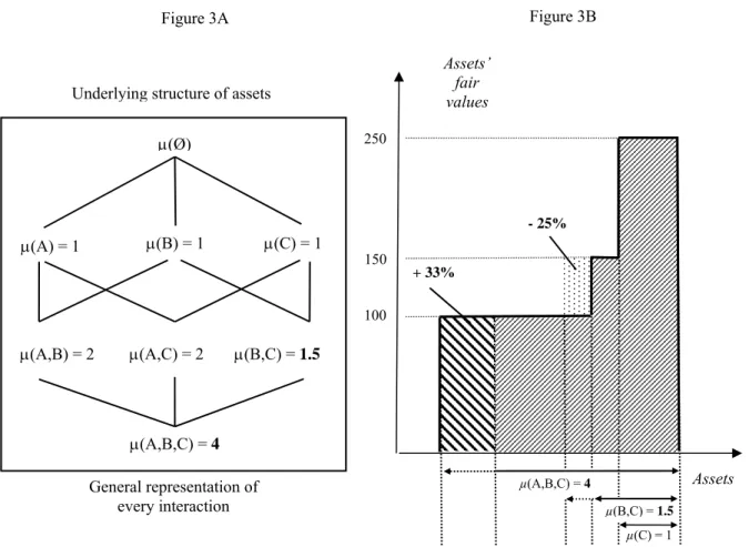
To reconcile individual fair values with the overall value of the firm, it is necessary to use other “measures” that model interactions between the assets of a firm and reflect the intensity of the relationship between sub-sets of assets. Consider a firm having a structured set X of three assets A, B, and C. We can graphically represent P(X), the power set of X (i.e., all possible combinations), in order to analyze the potential interactions (neutrality, synergy, inhibition) between the three assets (see Figure 3A). The change between Figure 2A and Figure 3A can be seen as mapping from the accounts-based representation to the non-additive representation of every possible interaction.
Insert Figure 3 About Here
As the actual structure of the economic reality is unknown, the most general form is assumed in the numerical representation, which exhibits every possible interaction between the three assets A, B, and C. At each node of the lattice, the interaction between two or three components can be reflected through the non-additive measure µ (defined below). The function µ captures the nature of the interaction between two or more assets. In other words, this function must offer special attributes for modelling (1) neutrality, (2) synergy, and (3) inhibition between assets.
Casta and Bry (1998; 2003) suggest using Choquet capacities (Choquet, 1953) instead of m as the non-additive measure µ. Choquet capacities are a generalization of the measure concept as they allow non-additive aggregation.
Choquet capacities respect a property called “monotonicity”, meaning that “adding a new item to a combination cannot decrease its importance” (Marichal, 2002, p. 3).6 This is a less constraining property than the additivity presented above. For two assets A and B, Choquet capacities can behave as follows, depending on the modelling requirement:
- Additive: (AB) (A)(B) (neutrality between assets) - Super-additive: (AB)(A)(B) (synergy between assets) - Sub-additive: (AB)(A)(B) (inhibition between assets).
The definition of Choquet capacities requires the measures of all subsets of X to be specified, that is to say 2n – 1 capacities to be estimated.7 This makes it possible to identify all the interactions between a set of assets.8
The Choquet aggregation stems directly from the capacities presented above. It is a generalization of the aggregation to non-additive measures.9 This approach allows non-additive aggregation of a set of assets where interactions between sub-sets of assets create (or destroy) value.
Firm Valuation under a Non-Additive Approach
The graphic illustration (see Figure 3) inspired by Murofushi and Sugeno (2000) provides a detailed presentation of the firm valuation method using the Choquet aggregation.
Graphic illustration of the additive approach (Figure 2B).
A firm has three assets A, B, and C ranked in order of increasing value. The fair values of these three assets are 100, 150, and 250 respectively. They can be represented by an increasing simple function f. The shaded area represents the overall fair value of the firm’s assets under the additive approach. The standard valuation approach requires computation of the area below the curve. The additive aggregation (equation (5)) of this simple function of assets is:
6 Let us assume two assets, individually worth 100 and 50. Monotonicity means that the value of the combination cannot fall below 100, i.e., the largest amount. This property can be relaxed empirically, allowing the value of the combination to take numbers below 100.
7 If X consists of n items, the number of items in P(X) is equal to 2n (includingthe empty set).
8 In a Statistical Transaction Theory approach, Hodgson et al. (1993, p. 143) similarly refer to the concept of “improper synergy elements”, which represent the various possible ways of combining the proper elements, i.e., the elements composing a set of assets. Hodgson et al. (1993, p. 143) consider the number of ways of partitioning a set of elements into nonempty sets following a Stirling number of the second kind.
9 According to Grabisch et al. (2009), the Choquet aggregation generalizes the Lebesgue integral (Lebesgue, 1918; Lebesgue, 1928) in the sense that the Choquet aggregation equals the Lebesgue integral when the capacities are additive (Marichal, 2002).
500 1 ) 150 250 ( 2 ) 100 150 ( 3 ) 0 100 ( ) ( ) 150 250 ( ) , ( ) 100 150 ( ) , , ( ) 0 100 ( ) ( ) ( 1 0 1 1
C m C B m C B A m S m s s V n i i i i Ad (5)where VAd represents the overall fair value of the assets based on the additive aggregation, Si is
the subset (combination) i of assets, si the (fair) value of the subset Si and m(Si) is an additive
measure of Si, representing the length of the intervals (see Figure 2B).
Graphic illustration of the Choquet capacity-based non-additive approach (Figure 3B). We now value the same firm, taking into account interactions between the assets using Choquet capacities. A learning process for estimating these capacities within a given industry is presented in the next section, but first let us assume that the capacities (i.e., each ) are known for this set of assets.
The Choquet capacities of the set of assets A, B, and C in this simplified example are: - µ(A) = µ(B) = µ(C) = 1; i.e., $1 of stand-alone asset value translates into $1 of enterprise
value in the structure;
- µ(A, B) = 2; i.e., neutrality between assets A and B (because µ(A, B) = µ(A) + µ(B)); - µ(A, C) = 2; i.e., neutrality between assets A and C (because µ(A, C) = µ(A) + µ(C)); - µ(B, C) = 1.5; i.e., 25% inhibition between assets B and C (because µ(B, C) < µ(B) + µ(C),
(i.e., (B, C)/[(B)+(C)] = 1.5/2 = 0.75, hence 25% of inhibition).
- µ(A, B, C) = 4; i.e., 33% synergy between assets A, B, and C (because µ(A, B, C) > µ(A)+ µ(B) + µ(C), i.e., (A, B, C)/[(A)+(B)+(C)] = 4/3 = 1.33, hence 33% of synergy).
For a firm having three assets with a given ranking of values, only three Choquet capacities are used to compute the overall firm value, because only three kinds of interaction are possible. Three other interaction coefficients would be used for another firm with another ranking of asset values. With many firms in a large sample and every possible ranking, seven capacities are possible with three assets. For example, if f(A) < f(B) < f(C), (A, B, C), (B, C), and (C) are required. If f(C) < f(A) < f(B), ( A, B, C), (A, B), and (B) are required, etc.
Compared with the additive approach, the non-additive method illustrated in Figure 3B can be seen as an extension (in the case of synergy) or contraction (in the case of inhibition) of the x-axis length of the area associated with every fair value difference below the curve (i.e., the measure m(.)). To represent the value of this structured set of assets graphically, the interaction value between assets A, B, and C (i.e., the synergy of 33%) is expressed by an extension of the x-axis length of the area associated with the 33% fair value difference for the three assets (i.e.,
from 3 to 4) resulting in the hatched area below the curve in Figure 3B. Furthermore, the inhibition between assets B and C is represented by a contraction of the x-axis length of the area associated with the 25% fair value difference between assets B and C (i.e., from 2 to 1.5) resulting in the dotted area below the curve. Hence, the new curve reflects the synergies and inhibitions between assets as expressed in Figure 3B.
The overall value of the firm calculated by a non-additive aggregation operator is equal to the shaded and hatched area below the new curve (in bold), i.e., the value of the Choquet aggregation. The capacities weigh the fair value differences for each combination of assets. The value of the Choquet aggregation (equation (6)) relative to the capacities for this set of assets is: 575 100 75 400 1 ) 150 250 ( 5 . 1 ) 100 150 ( 4 ) 0 100 ( ) ( ) 150 250 ( ) , ( ) 100 150 ( ) , , ( ) 0 100 ( ) ( ) ( 1 1 0 1 ) (
C C B C B A S s s C V n i i i i f C
(6)where VC represents the valuation based on the Choquet aggregation and µ(Si) is the Choquet
capacity of the subset Si.
In this illustration, both the synergies between the assets A, B, and C, and the inhibition between assets B and C are recognized. This leads to a new value of 575 for the firm (compared to only 500 with the additive approach).10
Estimation of Choquet Capacities11
It is necessary to define the value of 2n – 1 coefficients (S) where S represents one subset
among all the possible subsets (combinations) of assets. Similar to Grabisch et al. (2008), we suggest an indirect econometric method based on a regression model to estimate the coefficients. Determining the Choquet capacities (the 2n – 1 coefficients) involves a problem
for which many possible solutions have been put forward (Grabisch et al., 2008). We propose a specific estimation method using a sample made up of firms for which we have an estimate of the firm’s market value and the individual (book) value of each item in the set of assets.
10 Grabisch (1996, p. 451) offers a simple example of high school students’ grades where Choquet aggregation is explained as an average procedure that is capable of taking interaction between different high school subjects into account.
Since asset fair values are generally not disclosed, we use asset book values to address the issue of unrecognized intangible assets empirically.
For a sample of firms described by their overall enterprise value EV and a set of assets X, let f be the function assigning every subset S its monetary value s for each firm f :Ss. We define EV (the Enterprise Value) as:
EV := C(f) (7)
C(f) is the value of the Choquet aggregation and results from an analysis of asset interactions within the underlying activities.
The aim is to determine a set of Choquet capacities µ using a statistical procedure relying on market estimates of EV. We view market estimates as potential transaction costs for the set of activities, and do not assume perfect competition and a complete market (Gibbins and Willett, 1997).
Let S be a subset of P(X) and gS(f) be the function called generator, relative to the subset
S (when the assets have been ranked in value-increasing order) and defined as:12
1 0 1 ) ( ) ( n i i i S f s s g (8)The additive aggregation and Choquet non-additive aggregation can then be written as in equations (9) and (10), respectively:
) ( ) ( ) ( ) ( g f m S Ad X P S S f
(9) ) ( ) ( ) ( ) ( g f S C X P S S f
(10) Thus, according to equations (7) and (10) for a given sample, we can write the following econometric model, where for firm j:
) ( j j j ( ) ( ) EV X P S S f g S
(11)where (S) is now a parameter and is a residual which must be minimized in the estimation. The dependent variable is the enterprise value EV. The model given above is linear with 2n – 1
parameters: the (S) for all the subsets S of P(X). Using equation (11), the 2n – 1 coefficients
capture the non-additive effect of combining assets on firm value. The explanatory variables
12 This expression represents the difference in fair values of ranked assets and corresponds to the figures (100 – 0), (150 – 100) and (250 – 150) in the example of equations 5 and 6.
are the generators for each S corresponding to the value of the subsets of P(X). A standard OLS regression provides the estimation of these parameters, i.e., the required set of capacities.
Empirically, for each firm and subset S in P(X), we first compute the corresponding generator under equation (8). In the discrete case, the generator functions are merely the differences between the value of assets i+1 and i ranked by assets’ values. Next, to implement the model, for a sample of firms, we regress the enterprise value (dependent variable) on the generator functions (independent variables) for each subset of assets. The estimated coefficients are the Choquet capacities.
SAMPLE AND DATA
Our model is based on measuring interactions between assets. As interaction between assets can vary from one sector to another, we focus on a specific economic sector where synergies are likely to vary from one firm to another: the Capital Goods industry. It is important to balance sample size and homogeneity in a given sector, therefore we collect data for firms classified in the Capital Goods industry as defined by the Global Industry Classification Standard four-digit code GICS = 2010 (there are a total of 24 Industry Groups in the GICS classification). We collect data from COMPUSTAT North America over the period 1994 to 2014. Observations with missing variables are dropped from the sample. All continuous variables are winsorized at 1% and 99% to mitigate the effects of outliers. Our total sample is composed of 1,054 firms and 9,264 firm-year observations.
To implement the model, we group the identified assets into three broad classes: current assets (CA: accounts receivable, cash and cash equivalents, other current assets, tax assets), tangible assets (TA: PP&E, other tangible non-current assets) and intangible assets (IA: acquired brands, patents, etc.). Other classifications of assets could be used (e.g., business units, cash generating units). We make several important adjustments to these classes of assets.
Firstly, we remove cash and cash equivalents from current assets because cash is not an operating asset and there is little reason to expect that cash will interact with other asset classes. For the sake of consistency, we also subtract cash and cash equivalents in computing EV. Secondly, given the importance of unrecognized intangible assets, we also adjust intangible assets (IA). We include in IA an R&D capital asset computed as the past five years of R&D expenses assuming an annual amortization rate of 20% (Lev et al., 2005; Hirshleifer et al., 2013). Using a similar logic, we also include in IA an Advertising capital asset computed as the past five years of advertising expenses assuming an annual amortization rate
of 20%. Thirdly, we remove acquired (booked) goodwill from intangible assets for two reasons: (1) acquired goodwill was amortized until 2001 and subsequently tested for impairment (FASB, 2001b) which would lead to an inconsistent treatment of goodwill in our sample as it spans the period 1994-2014, (2) acquired goodwill potentially captures combination synergies between acquirer and target firms and IGG from purchased firms (see Figure 1), which we want to capture with the Choquet capacities.
Any synergies within a class of assets are captured by the coefficient on subsets of assets composed only of one individual class of assets (CA, TA and IA). For example, synergies between two intangible assets would lead to a greater capacity for that particular class of assets.13
Enterprise value is defined as market value of equity plus total liabilities minus cash and cash equivalents at the end of the fiscal year. Panel A of Table 1 presents the descriptive statistics for the full sample and subsamples based on size (large firms vs. small firms based on the median amount of total assets). Panel B presents descriptive statistics for the subsamples based on growth options (market-to-book ratio). We define the market-to-book ratio as enterprise value divided by adjusted total assets (= CA + TA + IA) instead of market value of equity divided by book value of equity, since our valuation model focuses on an asset-side approach that computes enterprise value as a non-additive aggregation of assets. Thus, our computation of the market-to-book ratio is similar to the notion of Tobin’s Q.
Insert Table 1 About Here
Panel A of Table 1 shows that the mean (median) market-to-book (EV/A) ratio is 1.84 (1.28) and is associated with a mean (median) IGG representing 16.8% (22.4%) of enterprise value. Mean (median) current assets account for 46.5% (45.7%) of total assets while tangible and intangible assets account for 29.5% (26.7%) and 13.0% (7.8%) respectively. The mean (median) Operating cash flows is -0.01% (6.8%) of total assets, and the mean (median) sales growth is 13.7% (6.8%).
Panel B of Table 1 indicates that firms have different characteristics depending on their market-to-book ratio. Firms with a market-to-book ratio below 0.90 have small but positive operating cash flows (mean operating cash flows of 1.2%) and lower sales growth relative to other firms (mean sales growth of 2.2% vs. 13.7% from Panel A in the full sample). Conversely, firms with a market-to-book ratio above 1.10 exhibit negative operating cash flows (mean
13 We acknowledge that working at a high level of aggregation (i.e., only the three classes CA, TA, and IA), means it is not possible to distinguish between a lower capacity between the classes and the possibility of individual assets within a class inhibiting the value of assets in another class.
operating cash flows of -2.2%) and strong sales growth (mean sales growth of 18.3%). Firms that have a market-to-book ratio between 0.90 and 1.10 theoretically provide a return on assets close to investors’ required rate of return, i.e., their ROA should be close to their (weighted average) cost of capital. The results will show that firms in the latter subsample have an underlying additive asset structure leading to limited or no interaction between assets.
EMPIRICAL RESULTS
Descriptive Statistics for Explanatory Variables: Generator Functions
We compute generator functions under equation (8) for each of the 9,264 firm-year observations. For each firm-year observation, the three asset classes are ranked in increasing order (Asset A < Asset B < Asset C). Next, each generator is computed in the following way: Asset A – 0 (generatorA,B,C), Asset B – Asset A (generatorB,C), Asset C – Asset B (generatorC).
This is simply a different way of describing a set of assets for a firm, and is convenient for estimating the Choquet capacities. As this equation is necessary (for estimation purposes), let us consider one firm in our sample: Boeing, having the following set of assets in 2013 (in millions of $): intangible assets (8,095), tangible assets (19,494) and current assets (65,074). Figure 4 provides a graphical representation of this set of assets ranked in increasing order.
Insert Figure 4 About Here
According to equation (8), we derive the value of the generators for Boeing Inc. as:
gIA,TA,CA = 8,095 – 0 = 8,095
gTA,CA = 19,494 – 8,095 = 11,399
gCA = 65,074 – 19,494 = 45,580
The other generators are equal to 0.14
Table 2 reports descriptive statistics for generator functions for the total sample, calculated in the same way as in the above example of Boeing, then scaled by total assets to standardize generators for the seven possible subsets (see above in Section 2 “Research Design”) and avoid estimated capacities being driven by large firms alone. For example, Table 2 shows that the mean (median) subset of assets composed of tangible assets and current assets is 16.4% (14.9%) of total assets. In the case of Boeing, the same subset of assets (generator gTA,CA) would
represent 11,399 / (8,095 + 19,494 + 65,074) = 12.3% of total assets.
14 Only three generators and three capacities are computed for each firm, since there are only three classes of assets. In the example of Boeing, IA < TA < CA, hence the computation of gTA,CA,IA, gTA,CA and gCA. For the sake of simplicity, the example uses Boeing’s assets unadjusted (as reported). We use adjusted assets for estimation purposes.
Insert Table 2 About Here Estimation of Choquet Capacities
Under the “learning” process presented in Section 2 and equation (11), the following equation is estimated for the whole sample in order to estimate the Choquet capacities:
j IAj CA TA IAj TA IAj CA CAj TA IAj CAj TAj j g g g g g g g EV
1
2
3
4 ,
5 ,
6 ,
7 , ,
(12)All variables are scaled by total assets. We do not include a constant in equation (12) because enterprise value is assumed to be equal to a (non-additive) combination of assets. Adding a constant would imply that enterprise value is associated with a constant factor across firms, independent of firms’ assets. We make the assumption that the value of a firm with no assets is zero. Estimation of the set of Choquet capacities for the sample is reported in Table 3.
Insert Table 3 About Here
Table 3 shows the estimated values, standard errors and p-values of Choquet capacities representing the value in the structure of every subset of assets for the full sample and the three subsamples based on the market-to-book ratio. The adjusted R² is reported although it has limited relevance in a regression without an intercept.15 We interpret the estimated capacities in the next paragraph.
Interpretation of Estimated Capacities
With three assets (TA, CA, and IA), we can explain the economic meaning of a capacity in the following way for the full sample (generators are scaled by total assets):
- (TA) = 3.198 means that an increase in tangible assets representing 1% of total assets would contribute to an increase in enterprise value representing 3.20% of total assets; - (CA) = 1.977 means that an increase in current assets representing 1% of total assets would
contribute to an increase in enterprise value representing 1.98% of total assets;
- (IA) = 6.535 means that an increase in intangible assets representing 1% of total assets would contribute to an increase in enterprise value representing 6.54% of total assets;
15 As explained above, we assume that a firm with no asset has a (non-additive) value of zero. This is also consistent with the nature of the Choquet’s integral according to which the value of the empty set is zero. However, the validity of this assumption depends on our adjustments to firms’ unrecognized assets.
- (TA, CA) = 2.690 means that an increase in tangible assets combined with current assets representing 2% of total assets would contribute to an increase in enterprise value representing 2.69% of total assets;
- (CA, IA) = 7.258 means an increase in current assets combined with intangible assets representing 2% of total assets would contribute to an increase in enterprise value representing 7.26% of total assets;
- (TA, IA) = 9.022 means that an increase in tangible assets combined with intangible assets representing 2% of total assets would contribute to an increase in enterprise value representing 9.02% of total assets;
- (TA, CA, IA) = 5.809 means that an increase in tangible assets combined with current assets and intangibles assets representing 3% of total assets would contribute to an increase in enterprise value representing 5.81% of total assets.
The estimated capacities can also be considered in terms of the marginal contributions of a particular subset to enterprise value. For two firms with the following asset structure (TA, CA, IA):
- Firm 1: (80, 200, 500) - Firm 2: (80, 200, 501)
The contribution of one extra dollar invested in intangible assets for firm 2 as compared to firm 1 is:
EV2(80, 200, 501) – EV1(80, 200, 500) = μ(IA) = 6.535 [See Table 3]
The enterprise value of firm 2 would be 6.54% of total assets higher than the enterprise value of firm 1. The same analysis can be performed for all the other combinations (e.g., (TA, CA, IA) = 5.809 means that the marginal contribution to enterprise value of investing 1% in each of a combination of TA, CA and IA is 5.81% of total assets.
The estimated capacities for our three subsamples exhibit very different patterns. For the subsample of firms with a market-to-book ratio close to one (between 0.90 and 1.10), the underlying asset structure is different from the industry’s average structure: estimated capacities exhibit an additive case, i.e., when the Choquet capacities are additive, as illustrated in Figure 3. Firms in this subsample do not generate positive interaction, nor do they generate negative interaction between their assets.
Conversely, capacities estimated for the subsamples that have a market-to-book ratio below 0.90 and above 1.10 exhibit specific non-additive underlying asset structures. The capacities of stand-alone assets estimated for firms with a market-to-book ratio below 0.90 are
lower than one, meaning that the marginal contributions of these subsets of assets to enterprise value are insufficient to recover their individual cost. In particular, the estimated capacities are lowest (0.36) for intangible assets, indicating that intangible assets fail to contribute significantly to enterprise value. For firms with a market-to-book ratio below 0.90, current assets have an estimated capacity of 0.72, which is the highest for single asset classes in this subsample and is consistent with the cash-type nature of these assets (e.g., accounts receivable). The value of the combination between TA and IA is also much lower for this subsample of firms relative to the other firms: only 1.10 vs. 9.02 in the full sample.
Firms with a market-to-book ratio above 1.10 exhibit a strikingly different pattern. First, the most valuable asset class appears to be IA with an estimated capacity of 9.10. These firms also exhibit very strong combinations between IA and CA and between IA and TA, with estimated capacities of 10.64 and 12.67, respectively.
Overall, the results show that the variation across the market-to-book ratio range is predominantly explained by the capacities of two subsets: intangible assets (estimated capacities for IA range from 0.36 to 9.10) and the combination of intangible assets and tangible assets (estimated capacities for (TA, IA) range from 1.10 to 12.67).
The Non-Additive Valuation Model and Firms’ Productive Efficiency
We assess the ability of our non-additive valuation approach to capture firm-specific productive efficiency in combining assets. The approach relies on a form of accounting production function. Industry and size are two important characteristics of production functions. Therefore, we consider two homogeneous size-based subsamples in the Capital Goods industry: Large Firms are defined as firm-year observations with total assets above the median, and Small Firms are defined as firm-year observations with total assets below the median. This leads to two subsamples of 4,632 (= 9,264/2) firm-year observations (see descriptive statistics in Panel A of Table 1). We estimate equation (12) for these two subsamples. The estimated coefficients, i.e., the Choquet capacities, provide the average productive efficiency for each type of observations, i.e., the market participants’ assessment of firm-year observations’ average capacity to generate economic benefits with a set of financial resources. Next, for every firm-year observation in the two subsamples, we compute the difference between:
(2) The value of the firm based on the average productive efficiency in the industry for each type of firm-year observation (estimated Choquet capacities for the appropriate type of firm-year observation) and its firm-specific set of assets:
_ , , _ , (13a)
_ , , _ , (13b)
where EVi,t is the current enterprise value for firm-year observation i at the end of fiscal year t
and _ , _ , is the predicted enterprise value given the estimated Choquet
capacities and firm-year observation i’s assets for a large (small) type of firm-year observation. Efficiency captures the market assessment of each firm-year observation’s specific productive efficiency relative to the average ability of firms in the industry to combine assets to generate economic benefits. This efficiency is likely to be persistent, because learning how to combine assets efficiently to generate economic benefits takes time. Lev et al. (2009) document that organization capital is associated with five years of future operating and financial performance. They refer to Evenson and Westphal (1995, p. 2237) to define organization capital as “the knowledge used to combine human skills and physical capital into systems for producing and delivering want-satisfying products”. We reason that our measure of productive efficiency based on the non-additive approach is likely to be correlated with organization capital, i.e., the ability to “convert resources into outputs” resulting in “super-normal performance” (Lev et al., 2009). Therefore, productive efficiency should also be positively associated with future realized operating performance.
We focus on two measures of operating performance: operating cash flows and sales growth. Operating cash flows is a core measure of operating performance but strong operating cash flows may only be realized after a given time period once the firm has reached sufficient maturity, depending on its business model and business cycle. Therefore, we also look at future sales growth capturing the potential ability to generate cash flows in later periods. This is particularly important for small firms which are more likely to be at earlier stages in their life cycles than larger firms.
We thus analyze future operating cash flows and sales growth for the three years following the valuation date. We analyze only three years of future performance in order to limit the loss of observations for our sample, which spans the period 1994-2014 (e.g., observations for t+3 are lost for observations from 2012). We estimate the following OLS model separately for large and small firm-year observations:
OCFi,t+k or ∆SALEi,t+k = b0 + b1Efficiencyi,t + b2OCFi,t or ∆SALEi,t + b3SIZEi,t
+ Year fixed effects + εi,t
(14)
where:
OCFi,t+k = net operating cash flows in t+1, t+2 and t+3 divided by total assets in
t;
∆SALEi,t+k = percentage change in sales computed for t+1, t+2 and t+3;
Efficiencyi,t = Efficiency_Larget or Efficiency_Smalli,t measured with equation (13)
depending on the appropriate firm type;
SIZEi,t = natural logarithm of total assets in t.
If our approach adequately captures observed productive efficiency, we expect Efficiency to be positively associated with future performance and b1 to be positive and significant. We include operating cash flows in fiscal year t (OCFt) and sales growth in fiscal year t (∆SALEi,t)
to control for autoregressive tendency. We also include firm size (SIZEi,t) which is likely to
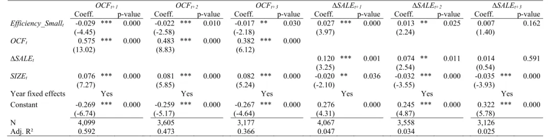
affect future performance. We include year fixed effects to control for business cycles. Estimation results are presented in Table 4.
Insert Table 4 About Here
Panel A of Table 4 shows that for large firms Efficiency is positively associated with future cash flows in t+1, t+2 and t+3 (significant at less than 5% or better, two-sided). Panel A also indicates that Efficiency is positively associated with future sales growth in t+1, t+2 and t+3 (significant at less than 5% or better, two-sided). These results indicate that the market assessment of these firms’ superior efficiency is realized in the form of higher future operating cash flows and stronger future sales growth.
Panel B of Table 4 presents the same analysis for less mature small firm-year observations. On average, for small firm-year observations, Efficiency is negatively associated with future operating cash flows in t+1, t+2, and t+3 (significant at less than 5% or better, two-sided) but positively associated with sales growth in t+1 and t+2 (significant at less than 5% or better, two-sided). These results indicate that the market assessment of these firms’ efficiency is not realized within three years, as operating cash flows are significantly lower for more efficient firms, but future performance is expected to be realized in later periods. The significant positive association between Efficiency_Small and sales growth in t+1 and t+2 indicates that the market assessment of small firms’ efficiency is associated with operating cash flows that will be realized in later periods, when these above-average growth firms reach maturity.
To assess how well the non-additive approach can estimate efficiency, we compare this approach with a simpler technique based on market-to-book ratio, which might be used to identify over- or under-efficient observations. Following the literature on the Tobin’s Q ratio (e.g., Servaes, 1991; Custodio, 2014), the market-to-book can also be used to investigate managerial ability to create value with a set of financial resources. We test the association between the market-to-book ratio and future performance with the OLS model (15):
OCFi,t+k or ∆SALEi,t+k = b0 + b1MTBi,t + b2OCFi,t or ∆SALEi,t + b3SIZEi,t
+ Year fixed effects + εi,t
(15)
where:
MTBi,t = market-to-book ratio of equity in t;
The other variables are as previously defined.
We include the same control variables as in model (14). We expect that MTB is positively associated with future cash flows and sales growth and a positive and significant b1 coefficient. Estimation results are presented in Table 5 for the subsamples of Large firms and Small firms.
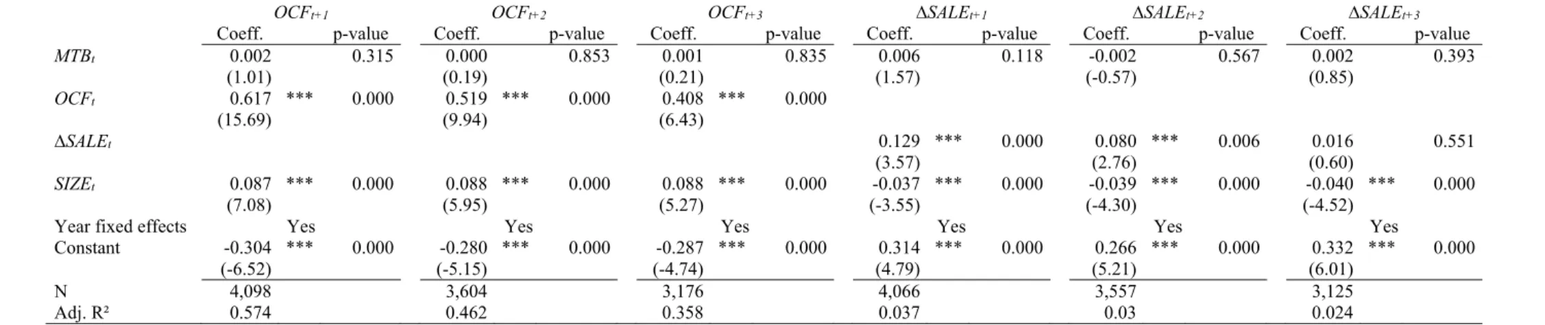
Insert Table 5 About Here
Panel A of Table 5 shows that for large firm-year observations market-to-book ratio (MTB) is positively associated with future cash flows in t+1, t+2, and t+3 (significant at less than 10% or better, two-sided). The market-to-book ratio is also positively associated with sales growth in t+1 and t+2 (significant at less 1%, two-sided). In addition, estimated coefficients b1 on the market-to-book ratio are economically small, ranging between 0.001 and 0.003.
Conversely, Panel B of Table 5 indicates that for small firm-year observations the market-to-book ratio exhibits no significant association with future performance (see insignificant b1 coefficient). In comparison, the non-additive approach (see Table 4, Panel B) appears better at identifying small firm-year observations with stronger future sales growth than an approach based on the market-to-book ratio. This is consistent with the argument that the non-additive valuation approach proves superior in identifying firms’ productive efficiency.
To make meaningful comparisons between the two approaches, we estimate the OLS model (16) that includes our measure of firm efficiency and the market-to-book ratio as independent variables likely to be associated with future operating performance:
OCFi,t+k or ∆SALEi,t+k = b0 + b1Efficiencyi,t + b2MTBi,t + b3OCFi,t or ∆SALEi,t
+ b4SIZEi,t + Year fixed effects + εt
(16)
where:
We reason that if the non-additive approach shows superior ability to measure firms’ production efficiency coefficient b1 would be positive and significant after controlling for the market-to-book ratio. Estimation results of model (16) are presented in Table 6.
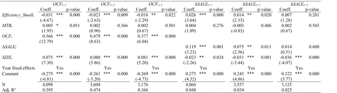
Insert Table 6 About Here
Panel A of Table 6 shows that for large firm-year observations Efficiency is positively associated with future operating cash flows in t+1, t+2 and t+3 (significant at less than 5% or better, two-sided) after controlling for the market-to-book ratio. We document a similar positive association between Efficiency and future sales growth in t+1, t+2 and t+3 (significant at less than 5% or better, two-sided) after controlling for the market-to-book ratio. We also find that after including our measure for efficiency the market-to-book is only marginally associated with future performance in t+1 (see b1 positive and significant at 10%, two-sided, when OCFt+1
is the dependent variable).
Panel B of Table 6 presents the estimation results of model (16) for small firms. We find that Efficiency is positively associated with future sales growth in t+1 and t+2 (significant at less than 5% or better, two-sided) after controlling for the market-to-book ratio of equity. Overall, the association between Efficiency and future performance is not affected by the inclusion of the market-to-book ratio. We find little evidence that the market-to-book ratio is able to measure productive efficiency among small firm-year observations. MTB is only positively associated with operating cash flows in t+1 (significant at less than 10%, two-sided).
Overall, our non-additive valuation approach measures firms’ ability to combine assets relatively to the average firm in the industry. Our measure of efficiency is associated with future operating cash flows (Large firms) or sales growth (Small firms) in a predictable pattern. Our approach appears to be better able to identify expected relationships between efficiency and future performance than a simpler approach based on the market-to-book ratio.
DISCUSSION AND CONCLUSION
Firms are efficient organizations that combine assets in order to generate synergies creating super-profits. It is thus inappropriate to value a firm made up of several interdependent assets simply by summing the individual values of those assets, because the aggregation function ignores interdependencies. Miller (1973) and Gibbins and Willett (1997) identified this approach as stemming from an inappropriate theory of aggregation in accounting. Existing valuation methods do not use individual asset values, but compute enterprise value under additive aggregation functions focusing on discounted future cash flows (DCF) or abnormal
earnings (RIM). We suggest that the aggregation issue can be addressed by introducing a non-additive aggregation function. Our approach is able to reconcile enterprise value with the value of assets in place.
To explain our approach, we study the relationship between market-to-book ratio and estimated Choquet capacities. We estimate our technique for a sample of 9,264 firm-year observations and show that a predictable pattern of association exists between estimated Choquet capacities and the market-to-book ratio. We also find that our valuation approach is better able to measure a firm’s productive efficiency than a simple approach based on the median market-to-book ratio for the industry concerned.
Our approach relies on a limited amount of information and could easily be applied to value private firms for which forecast data is not widely available. It is important to consider the trade-off between the degree of homogeneity of the peer group and its size. The non-additive model could also be used to analyze the synergies (or redundancies) between multiple-business-segment firms as business segment data becomes available (e.g., Compustat segments).
The technique we propose could be refined. It would be possible to analyze further the appropriate level of aggregation at which to examine interactions between assets, such as business units or cash-generating units instead of the three asset classes used in this study. The analysis could also be extended to consider more than three asset classes.
From a conceptual standpoint, estimating the non-additive model by reference to book value accounting is a simplification of fair value. As we consider that the balance sheet correctly represents the stand-alone market value of assets for our sample, the role of synergies may be overstated if there are unidentified intangible assets or, more generally, understated assets (although we make several adjustments for unrecognized intangible assets). This drawback could be overcome by using the fair value estimates disclosed in purchase price allocations (PPAs) under the acquisition method of accounting for business combinations, which has been mandatory since 2002 in the U.S. (FASB, 2001a). However, the limited availability of PPA data (dependent on an acquisition having taken place, and disclosure of the PPA by acquiring firms) would considerably limit sample size.
The additivity assumption is a stabilized implicit hypothesis that is often unquestioningly accepted in financial accounting. It provides an “invisible” management instrument (Hatchuel and Weil, 1995) that may restrict the way organizations are perceived and managed. By relaxing the additive postulate, this paper not only suggests a new way to value firms but also attempts to broaden the debate on the role of additivity in management.
REFERENCES
Arnold, J., D. Eggington, L. Kirkham, R. Macve and K. Peasnell, 'Goodwill and Other Intangibles: Theoretical Considerations and Policy Issues', Institute of Chartered Accountants in England and Wales, 1994.
Barth, M. E., W. H. Beaver, J. R. M. Hand and W. R. Landsman (2005), 'Accruals, Accounting-Based Valuation Models, and the Prediction of Equity Values', Journal of Accounting, Auditing & Finance, Vol. 20, No. 4, pp. 311-345.
Beyer, A., D. A. Cohen, T. Z. Lys and B. R. Walther (2010), 'The Financial Reporting Environment: Review of the Recent Literature', Journal of Accounting and Economics, Vol. 50, No. 2-3, pp. 296-343.
Bloom, M. (2009), 'Accounting for Goodwill', Abacus, Vol. 45, No. 3, pp. 379-389. Canning, J. B. (1929), The Economics of Accountancy, The Ronald Press Company.
Casta, J.-F. and X. Bry (1998), 'Synergy, Financial Assessment and Fuzzy Integrals', In Proceedings of IVth Congress of International Association for Fuzzy Sets Management and Economy (SIGEF) Santiago de Cuba, pp. 17-42.
Casta, J.-F. and X. Bry (2003), 'Synergy Modelling and Financial Valuation: The Contribution of Fuzzy Integrals', In Connexionist Approaches in Economic and Management Sciences (Eds, Cotrel, M. and Lesage, C.) Kluwer Academic Publishers, pp. 165-182. Choquet, G. (1953), 'Théorie Des Capacités', Annales de l’institut Fourier, Vol. 5, pp. 131-295. Custodio, C. (2014), 'Mergers and Acquisitions Accounting and the Diversification Discount',
Journal of Finance, Vol. 69, No. 1, pp. 219-240.
Evenson, R. E. and L. E. Westphal (1995), 'Technological Change and Technological Strategy', In Handbook of Development Economics, Vol. 3, Part 1 (Eds, Behrman, J. and Srinivasan, T. N.) North-Holland.
FASB (2001a), Statement of Financial Accounting Standards (SFAS) No. 141: Business Combinations, Financial Accounting Standards Board, Norwalk, CT.
FASB (2001b), Statement of Financial Accounting Standards (SFAS) No. 142: Goodwill and Other Intangible Assets, Financial Accounting Standards Board, Norwalk, CT.
Gibbins, M. and R. J. Willett (1997), 'New Light on Accrual, Aggregation and Allocation, Using an Axiomatic Analysis of Accounting', Abacus, Vol. 33, No. 2, pp. 137.
Gilboa, I. (1988), 'A Combination of Expected Utility and Maxmin Decision Criteria', Journal of Mathematical Psychology, Vol. 32, No. 4, pp. 405-420.
Grabisch, M. (1996), 'The Application of Fuzzy Integrals in Multicriteria Decision Making', European Journal of Operational Research, Vol. 89, pp. 445-456.
Grabisch, M., I. Kojadinovic and P. Meyer (2008), 'A Review of Methods for Capacity Identification in Choquet Integral Based Multi-Attribute Utility Theory: Applications of the Kappalab R Package', European Journal of Operational Research, Vol. 186, No. 2, pp. 766-785.
Grabisch, M., J.-L. Marichal, R. Mesiar and E. Pap. (2009), Aggregation Functions, Cambridge University Press, New York.
Gynther, R. S. (1969), 'Some 'Conceptualizing' on Goodwill', The Accounting Review, Vol. 44, No. 2, pp. 247-255.
Hatchuel, A. and B. Weil (1995), The Expert and the System, de Gruyter, Berlin.
Henning, S. L., B. L. Lewis and W. H. Shaw (2000), 'Valuation of the Components of Purchased Goodwill', Journal of Accounting Research, Vol. 38, No. 2, pp. 375-386. Hirshleifer, D., P.-H. Hsu and D. Li (2013), 'Innovative Efficiency and Stock Returns', Journal
of Financial Economics, Vol. 107, No. 3, pp. 632-654.
Hodgson, A., J. Okunev and R. Willett (1993), 'Accounting for Intangibles: A Theoretical Perspective', Accounting & Business Research, Vol. 23, No. 90, pp. 138-150.