A unified formalism for complex systems architecture

HAL Id: pastel-00827107

https://pastel.archives-ouvertes.fr/pastel-00827107v2

HAL is a multi-disciplinary open access

archive for the deposit and dissemination of sci-entific research documents, whether they are pub-lished or not. The documents may come from teaching and research institutions in France or

L’archive ouverte pluridisciplinaire HAL, est destinée au dépôt et à la diffusion de documents scientifiques de niveau recherche, publiés ou non, émanant des établissements d’enseignement et de recherche français ou étrangers, des laboratoires

Boris Golden

To cite this version:

Boris Golden. A unified formalism for complex systems architecture. Modeling and Simulation. Ecole Polytechnique X, 2013. English. �pastel-00827107v2�

A Unified Formalism for

Complex Systems Architecture

Ph.D. in Computer Science

by

Boris

Golden

Defended on May 13th 2013 in front of:

M. Daniel KROB Ecole Polytechnique´ Advisor

M. Marc AIGUIER Ecole Centrale Paris (ECP)´ Co-Advisor

M. Fr´ed´eric BOULANGER Sup´elec Reporter

M. Sylvain PEYRONNET Universit´e de Caen Reporter M. Marc POUZET Ecole Normale Sup´erieure (ENS)´ Reporter

M. ´Eric GOUBAULT CEA President

M. Patrice PERNY Universit´e Paris 6 Examiner

´

Acknowledgments

Thank you to Daniel Krob, who introduced me to the fascinating subject of systems architecture, from formal models to real industrial case studies!

Thank you to Marc Aiguier, who helped me make all this happen, and who has been supportive during the whole study!

Thank you to Dan Frey for inviting me to visit him at the Massachusetts Institute of Technology, opening new perspectives for my work!

Thank you to Antoine Rauzy who has always been providing stunning in-sights & feedbacks on my work!

Thank you to Patrice Perny for introducing me to the amazing world of multi-criteria optimization!

Thank you to Yann Hourdel with whom I have been working at LIX and sharing a lot at the end of my PhD!

Thank you to Fr´ed´eric Boulanger, Sylvain Peyronnet and Marc Pouzet for accepting to be the reporters of this PhD thesis!

Thank you to ´Eric Goubault for having accepted to be the President of the Jury for my defense!

Thank you to my friends and family who have provided so much support during my whole PhD!

Abstract

Complex industrial systems are typically artificial objects designed by men, involving a huge number of heterogeneous components (e.g. hardware, software, or human organizations) working together to perform a mission. In this thesis, we are interested in modeling the functional behavior of such systems, and their integration. We will model real systems as functional black boxes (with an internal state), whose structure and behaviors can be described by the recursive integration of heterogeneous smaller subsystems.

Our purpose is to give a unified and minimalist semantics for heterogeneous integrated systems and their integration. By “unified”, we mean that we propose a unified model of real systems that can describe the functional behavior of heterogeneous systems and that is closed under integration. By “minimalist” we mean that our formalization intends to provide a small number of concepts and operators to model the behaviors and the integration of complex industrial systems. Our work thus allows to give a relevant formal semantics to concepts and models typically used in Systems Engineering.

In this framework, the integration of real systems can be modeled as a re-cursive process consisting in alternating composition and abstraction, to build a target overall system from elementary systems recursively composed and ab-stracted at different levels. Based on these definitions of systems and their integration, a minimalist systems architecture framework allows to deal with requirements, systems structure and underspecification during the design.

In this thesis, we first define heterogeneous dataflows, and then systems as step-by-step machines transforming dataflows. Such systems can be integrated using operators, to build more complex systems, so that we can handle the two dimensions of the complexity (heterogeneity and integration). We then in-troduce a minimalist formalism for systems architecture to model requirements, underspecification & structure of systems through the design process. We finally open perspectives around systems optimization when fairness is required. Keywords: Complex industrial systems, Systems modeling, Systems archi-tecture, Systems semantics, Systems Engineering, Systems integration, Timed Mealy machine, Hybrid time, Non-standard analysis, Dataflows, Architecture framework, Transfer function, Requirements, Fair optimization.

l’Homme, et constitu´es d’un grand nombre de composants h´et´erog`enes (e.g. mat´eriels, logiciels ou organisationnels) collaborant pour accomplir une mission globale. Dans cette th`ese, nous nous int´eressons `a la mod´elisation du comporte-ment fonctionnel de tels syst`emes, ainsi qu’`a leur int´egration. Nous mod´eliserons donc les syst`emes r´eels par le biais d’une approche de boˆıte noire fonctionnelle avec un ´etat interne, dont la structure et le comportement fonctionnel peuvent ˆetre obtenus par l’int´egration r´ecursive de composants ´el´ementaires h´et´erog`enes. Notre but est de donner une s´emantique unifi´ee et minimaliste pour de tels syst`emes, ainsi que pour leur int´egration. Par “unifi´e”, nous voulons dire que nous proposons un mod`ele permettant de repr´esenter diff´erents types de syst`emes et qui reste clos sous les op´erateurs d’int´egration. Par “minimaliste”, nous voulons dire que notre formalisme entend d´efinir un petit nombre de con-cepts et d’op´erateurs pour mod´eliser l’int´egration des syst`emes industriels com-plexes. Notre travail permet donc de donner une s´emantique aux concepts et mod`eles typiquement utilis´es en Ing´enierie syst`eme.

Dans ce cadre, l’int´egration de syst`emes r´eels peut ˆetre mod´elis´ee comme un processus r´ecursif consistant en une alternance de composition et d’abstraction, pour construire un syst`eme cible `a partir de syst`emes plus ´el´ementaires r´ecursive-ment connect´es entre eux puis red´efinis `a des niveaux sup´erieurs d’abstraction. En s’appuyant sur ces d´efinitions, nous proposons un cadre d’architecture mini-maliste qui permet d’exprimer des exigences, de d´ecrire la structure d’un syst`eme et de rendre compte de la sous-sp´ecification durant la phase de conception.

Dans cette th`ese, nous d´efinissions tout d’abord la notion de flots de donn´ees h´et´erog`enes, puis de syst`emes comme machines de transformation de flots de donn´ees de fa¸con algorithmique. Ces syst`emes peuvent ensuite ˆetre int´egr´es par le biais d’op´erateurs, permettant de construire des syst`emes plus complexes, et donc de rendre compte des deux dimensions principales de la complexit´e (l’h´et´erog´en´eit´e et l’int´egration). Nous introduisons ensuite un formalisme pour l’architecture syst`eme, en mod´elisant les exigences, la sous-sp´ecification et la structure des syst`emes. Enfin, nous ouvrons des perspectives autour de l’optimi-sation entre syst`emes lorsque l’´equit´e est recherch´ee.

Mots-cl´es : Syst`emes industriels complexes, Mod´elisation de syst`eme, Archi-tecture syst`eme, S´emantique des syst`emes, Ing´enierie syst`eme, Int´egration de syst`emes, Machine de Mealy temporis´ee, Temps hybride, Analyse non-standard, Flot de donn´ees, Cadre d’architecture, Fonction de transfert, Exigences, Opti-misation ´equitable.

Contents

1 Introduction 9

1.1 Complex industrial systems . . . 9

1.2 Systems Engineering . . . 11

1.3 What is systems architecture? . . . 13

1.3.1 A definition . . . 13

1.3.2 Fundamental principles . . . 15

1.4 Towards a unified formalism . . . 19

1.5 Structure of this manuscript . . . 21

I

Systems modeling

23

2.2.2 Implementation of standard data behaviors . . . 32

2.3 Dataflows . . . 33 2.3.1 Definition . . . 33 2.3.2 Operators . . . 33 2.3.3 Consistency of dataflows . . . 35 3 Systems 39 3.1 Systems . . . 39 3.1.1 Definition . . . 39 3.1.2 Execution . . . 41

3.1.3 Examples & expressivity . . . 42

3.2 Transfer functions . . . 45

3.2.1 Definition . . . 46

4 Integration operators 49 4.1 Composition . . . 49 4.1.1 Timed extension . . . 50 4.1.2 Product . . . 52 4.1.3 Feedback . . . 55 4.2 Abstraction . . . 57 4.2.1 Nondeterminism . . . 58 4.2.2 Abstraction . . . 59 4.3 Integration of systems . . . 61

4.3.1 Composition & abstraction . . . 61

4.3.2 Example . . . 62

II

Systems architecture

65

5.1.1 Preliminaries . . . 67

5.1.2 Transfer functions via coalgebras . . . 69

5.1.3 Systems as coalgebras . . . 70

5.2 A logic for system requirements . . . 72

5.2.1 Definition . . . 72

5.2.2 Examples of requirements . . . 74

5.2.3 Adequacy of the logic . . . 76

6 Towards a framework for systems architecture 79 6.1 Handling underspecification . . . 80

6.2 Modeling recursive structure . . . 83

7 Fair assignments between systems 89 7.1 Introduction . . . 90

7.2 Inequality measurement with Lorenz dominance relations . . . . 92

7.2.1 Notations and definitions . . . 92

7.2.2 Infinite order Lorenz dominance . . . 95

7.3 Properties of infinite order Lorenz dominance . . . 97

7.3.1 A representation theorem . . . 97

7.3.2 Main properties of L∞-dominance . . . 100

7.4 Solving multiagent assignment problems . . . 102

7.4.1 Fair multiagent optimization . . . 103

7.4.2 Linearization of the problem . . . 104

7.4.3 Numerical tests . . . 105

Chapter 1

Introduction

1.1

Complex industrial systems

Industrial systems are typically artificial objects designed by men, involving heterogeneous components (mostly: hardware, software, and human organiza-tions) working together to perform a mission. In this thesis, we are interested in modeling the functional behavior of such systems, and their integration. From a practical point of view, our aim is to give a unified formal semantics to the concepts manipulated on a daily basis by engineers from various fields working together on the design of complex industrial systems. Indeed, they need formal tools to reason on & model those systems in a unified & consistent way, with a clear understanding of the underlying concepts.

We will model complex industrial systems as heterogeneous integrated sys-tems, since our work highlights two aspects of the complexity of such systems:

• the heterogeneity of systems, that can be naturally modeled following continuous or discrete time, and that are exchanging data of different types1. Several specialized fields are involved in the design of a complex industrial system, making it difficult to keep a unified vision of this system and to manage its design.

• the integration of systems, i.e. the recursive mechanism to build a system through the synthesis of smaller systems working together, and whose be-haviors will be described at a more concrete level (i.e. a finer grain). There are many interrelations between a possibly huge number of components, and there are recursive levels of integration.

The concept of complex systems has led to various definitions in numerous disciplines (biology, physics, engineering, mathematics, computer science, etc).

1

Data encompasses here all kinds of elements that can be exchanged between real objects. We distinguish three kinds of homogeneous systems: hardware/physical systems (transforming continuous physical parameters), software systems (transforming and managing discrete data), and human/organizational systems (organized through processes).

One speaks for instance of dynamical, mechanical, Hamiltonian, hybrid, em-bedded, concurrent or distributed systems (cf. [6, 8, 45, 53, 60]). A minimalist informal definition consistent with (almost) all those of the literature is that a system is “a set of interconnected parts forming an integrated whole”, and the adjective complex implies that a system has “properties that are not easily understandable from the properties of its parts”. In the mathematical formal-ization of complex systems, there are today two major approaches: the first one is centered on understanding how very simple but numerous elementary com-ponents can lead to complex overall behaviors (e.g. cellular automatas), the second one (that will also be ours) is centered on giving a precise semantics to the notion of system and to the integration of systems to build greater overall systems.

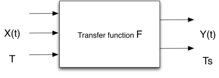
When mathematically apprehended, the concept of system (in the sense of this second approach) is classically defined with models coming from:

• control theory and physics, that deal with systems as partial functions (dynamical systems may also be rewritten in this way), called transfer functions, of the form:

∀t ∈ T, y(t) = F (x, q, t)

where x, q and y are inputs, states and outputs dataflows, and where T stands for time (usually considered in these approaches as continuous (see [60, 5, 21]).

• theoretical computer sciences and software engineering, with systems that can be depicted by automaton-oriented formalisms equivalent to timed transition systems with input and output, evolving on discrete times gen-erally considered as a universal predefined sequence of steps (see for in-stance [37, 10, 35, 26, 19, 18]). There is also a purely logical approach for representing discrete abstract systems. The core modelling language in this direction is probably Lustre [35, 20]. A reasoned overview of all these approaches can be found in [39].

However all these models do not easily allow to handle systems with het-erogeneous time scales. The introduction of a more evolved notion of time within models involves many difficulties, mainly the proper definition of sequen-tial transitions or the synchronization of different systems exchanging dataflows without synchronization of their time scales. Dealing with an advanced defi-nition of time will typically imply to introduce infinity and infinitesimal (for instance with non-standard real numbers).

To address this challenge, the theory of hybrid systems was developed jointly in control theory (see [60, 66]) and in computer science (see [36, 6, 41]). A serious issue with this theory is however that the underlying formalism has some troubling properties such as the Zeno’s paradox which corresponds to the fact that an hybrid system can change of state an infinite number of times within a finite time with the convergence of a series of decreasing durations

1.2. SYSTEMS ENGINEERING which should be avoided in a robust modeling approach. Other interesting and slightly different attempts in the same direction can also be found in Rabinovitch and Trakhtenbrot (see [52, 61]) who tried to reconstruct a finite automata theory on the basis of a real time framework, or in [67]. Hybrid automatas (see [36]) are another classical model for representing abstract hybrid systems.

Moreover, none of these models address the integrative & architectural di-mensions of complex industrial systems (an approach similar to ours on the structure of complex systems, but without the introduction of heterogeneous time, has been carried out in [3], using a coalgebraic formalism). There is therefore a great challenge on being able to unify in a same formal framework mathematical methods dealing with the definition & design of both continuous and discrete systems, and at the same time being able to define the integration & architecture of such systems in the same formalism. This will be at the center of our approach.

1.2

Systems Engineering

When dealing with complex industrial systems containing heterogeneous com-ponents, engineers face problems with the semantics of the models they work with to describe real systems when they involve a large number of heterogeneous elementary systems.

To build modern industrial systems, it has thus been necessary to create complex engineering models & processes being able to deal with a huge number of engineers coming from many different domains. Indeed, because of the size of such modern industrial systems (trains, planes, space shuttles, etc), their real-ization leads to major conceptual and technical difficulties. The reason is that it is difficult, or even impossible, for one single person to completely comprehend such systems globally. Although this designation is not precise nor universal, it is naturally associated with industrial systems whose design, industrialization and change lead to important and difficult problems of integration, directly related to both the huge number of basic components integrated at multiple levels, and the important scientific and technological heterogeneity of such systems (gener-ally involving software, hardware/physical and human/organizational parts). To manage the complexity of such systems, some methods have emerged during the last century. We can trace the origin of these methods to the Cold War where USA had to build defence systems for which the issues of data manage-ment, decisions and military riposte had been taken into account as a whole, in an integrated and consistent way, in order to ensure a short reaction time between a Soviet attack and an American counter-attack. From there, a body of knowledge called Systems Engineering, focused on the integration mastery of large industrial systems has progressively emerged since the 50’s. Hence, Sys-tems Engineering consists of a set of concepts, methods and good organizational and technical practices that the industry had to develop to be able to deal with the complexity of industrial systems (see [11, 42, 57, 62] for more details on this subject).

But in fact, Systems Engineering is “just” the application to engineering of a more general thought paradigm, called systems approach (also often referred to as systems thinking). Systems approach focuses on interactions between sys-tems, and views such systems as black boxes described only through their func-tional behavior and their internal state. In systems approach, a system is thus a black box receiving and emitting flows, and characterized by an internal state. A system can itself be decomposed into a set of interconnected subsystems. It is therefore an observational modeling of systems. Systems approach also implies to step back with a high-level point of view seeing any system as being part of an overall greater system (i.e. a system is in interaction with other systems in its environment).

A key assumption of systems approach is thus to consider that any system is only in interaction with other systems, and that the behavior of any real system2 _{can be explained within this framework. The main advantage of this}

approach is that it helps to understand how things influence one another within a whole (with often unexpected long-term or long-distance influences). All inter-actions between systems are captured by logical flows, figuring a unidirectional transmission of elements (which can be material, energetic or informational). “Logical” here means that it only models the exchange of data between ele-ments, and not the way this exchange really occurs. For instance, the physical reality behind a flow between two real systems (like the delay or the rate of transmission of the network cable between two computers) will itself be mod-eled by a specific type of system called interface (it would here take into account the physical properties of the cable, when the flow would only account for the logical exchange of data).

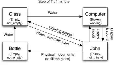
The systems approach is a very powerful tool to model a lot of real-life objects and situations. We give a simple example to illustrate the main concepts of systems approach. Imagine an individual, John, sitting in front of its computer and using it. John has on its table a bottle of water and a glass he uses when he is thirsty. We want to model the overall real system3 _{(which is here closed,}

i.e. not exchanging data with its environment). We should characterize the following objects at the right abstraction level:

• systems: those are all the objects involved. Here: glass, bottle, computer, John (the table will not be useful in our modeling).

• states: each system has a set of possible states. E.g. the glass can be ‘not empty’ or ‘empty’.

2

In the literature, the real object and its model are often confused and both called system. When clarification is needed, we will call real system any object of the real world which behavior we want to explain as a transformation of flows of data. We will call system the mathematical object introduced to model real systems.

3_{As every model, it is not exhaustive since focused on given aspects of the real system}

1.3. WHAT IS SYSTEMS ARCHITECTURE? • data: each system can receive or send data. E.g. the glass can send water,

or a visual stimulus (indicating the level of water in the glass).

• flows: each system has inputs and outputs that allow it to exchange data with other systems. E.g. the bottle can send water to the glass (when the bottle is not empty). But the glass may send water to the computer, even if it is not its intended use.

• behaviors (functions and states): each system will have specific behaviors that will make it generate outputs and change its states, according to time and inputs. E.g. when the glass is empty and receives water, it becomes not empty. But if it receives a drinking move, it sends water to John and becomes empty.

• time of the overall system: a time scale of description has to be chosen to be consistent with the model. E.g. a step of 1 minute for the time scale can be a consistent choice here.

Bottle

Glass

John

Computer

Water

Water Water_{, visual stimulus}

Drinking moves

Physical movements (to fill the glass)

Display & sound User's inputs {Broken, working} {Empty, not_empty} {Thirsty, not_thirsty} Step of T : 1 minute {Empty, not_empty}

Figure 1.1: Example of an elementary systemic modeling

All the concepts introduced here are informal. We will give a semantics to all the objects of this intuitive “graphical” language used in systems approach.

1.3

What is systems architecture?

1.3.1

A definition

Systems Architecture is a generic discipline to handle systems (existing or to be created), in a way that supports reasoning about the structural properties of these objects.

• the architecture of a system, i.e. a model to describe/analyze a system • architecting a system, i.e. a method to define the architecture of a system • a body of knowledge for ”architecting” systems while meeting business

needs, i.e. a discipline to master systems design.

At this point, we can only say that the ”architecture of a system” is (similarly to the one of a building) a global model of a real system consisting of:

• a structure

• properties (of various elements involved) • relationships (between various elements) • behaviors & dynamics

• multiple views of elements (complementary and consistent).

We will not describe here the numerous issues raised (at every level of a com-pany: corporate strategy, marketing, product definition, engineering, manufac-turing, operations, support, maintenance, etc) by the design and management of complex industrial systems. But these issues can be summarized as:

• going from local to global, i.e. mastering integration and emergence • building an invariable architecture in a moving environment.

In this context, Systems Architecture is a response to the conceptual and practical difficulties of the description and the design of complex industrial sys-tems. Systems Architecture helps to describe consistently and design efficiently complex systems such as:

• an industrial system (the original meaning of Systems Architecture) • an IT infrastructure (Enterprise Architecture)

• an organization (Organizational Architecture) • a business (Business Architecture).

Systems Architecture will often rely on a tool called an architecture frame-work, i.e. a reference model to organize the various elements of the architecture of a system into complementary and consistent predefined views allowing to cover all the scope of Systems Architecture. Famous architecture frameworks are for instance: DoDAF, MoDAF or AGATE4_.

Finally, Systems Architecture will consider any system with a socio-technical approach (even when dealing with a ”purely” technical system). In particular, during the design (or transformation) of a system, the systems in the scope of this design (or transformation) can be divided in two separated systems in interaction:

4_{A good overview of these frameworks can be found on Wikipedia:}

1.3. WHAT IS SYSTEMS ARCHITECTURE? • the product, i.e. the system being designed or transformed

• the project, i.e. the socio-technical system (teams, tools, other resources and their organization following strategies & methods) in charge of the design or transformation of the product.

1.3.2

Fundamental principles

Whatever the type of system and the acception considered (model, method or discipline), Systems Architecture is based on 9 fundamental principles:

Thinking with a systemic approach

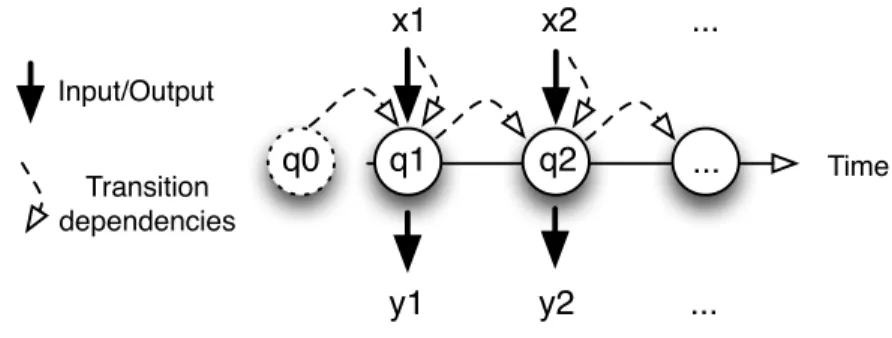
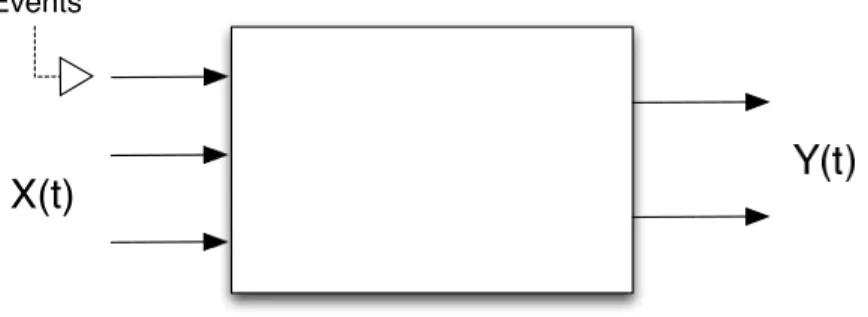
1. the objects of the reality are modeled as systems (i.e. a box performing a function and defined by its perimeter, inputs, outputs and an internal state). Ex: a mobile phone is a system which takes in input a voice & keystrokes and outputs voices & displays. Moreover, it can be on, off or in standby. Overall, the phone allows to make phone calls (among other functions).

Q

...

_...

Y

X

2. a system can be broken down into a set of smaller subsystems, which is less than the whole system (because of emergence). Ex: a mobile phone is in fact a screen, a keyboard, a body, a microphone, a speaker, and electronics. But the phone is the integration of all those elements and cannot be understood completely from this set of separate elements.

3. a system must be considered in interaction with other systems, i.e. its environment. Ex: a mobile phone is in interaction with users, relays (to transmit the signal), repairers (when broken), the ground (when falling), etc. All these systems constitute its environment and shall be considered during its design.

S

4. a system must be considered through its whole lifecycle. Ex: a mobile phone will be designed, prototyped, tested, approved, manufactured, dis-tributed, sold, used, repaired, and finally eventually recycled. All these steps are important (and not only the moment when it is used).

1

2

3

4

S(1)

S(2)

S(3)

S(4)

Reasoning according to an architecture paradigm

5. a system can be linked to another through an interface, which will model (when needed) the properties of the way they are linked in the reality. Ex: when phoning, our ear is in direct contact with the phone, and there is therefore a link between the two systems (the ear and the phone). However, there is a hidden interface: the air! The properties of the air may influence the link between the ear and the phone (imagine for example if there is a lot of outside noise).

1.3. WHAT IS SYSTEMS ARCHITECTURE?

interface

6. a system can be considered at various abstraction levels, allowing to con-sider only relevant properties and behaviors. Ex: do you concon-sider your phone as a device to make phone calls (and other functions of modern phones), a set of material and electronics components manufactured to-gether, or a huge set of atoms ? All these visions are realistic, but they are just at different abstraction levels, whose relevancy will depend on the purpose of the modeling.

abstraction

7. a system can be viewed according to several layers (typically three at least: its purpose, its functions, and its construction). Ex: a phone is an object whose purpose is to accomplish several missions for its environment: making phone calls, being a fashionable object, offering various features of personal digital assistants, etc. But it is also a set of functions organized to accomplish these missions (displaying on the screen, transmitting signal, delivering power supply, looking for user inputs, making noise if necessary, etc). And finally, all these functions are implemented through physical components organized to perform these functions.

Why ? = purpose

What ? = functions

How ? = composition

8. a system can be described through interrelated models with given seman-tics (properties, structure, states, behaviors, datas, etc). Ex: from the point of view of properties, the phone is a device expected to meet require-ments like ”a phone must resist to falls from a height of one meter”. But a phone will also change state: when a phone is off and that the power but-ton is pressed, the phone shall turn on. Function dynamics of the phone are also relevant: when receiving a call, the screen will display the name and the speaker will buzz, but if the user presses no button the phone will stop after 30 seconds... This will typically be described with diagrams in modeling languages like UML or SysML.

9. a system can be described through different viewpoints corresponding to various actors concerned by the system. Ex: marketers, designers, engi-neers (in charge of software, electronics, acoustics, materials, etc), users, sales, repairers... All these people will have different visions of the phone. When the designer will see the phone as an easy-to-use object centered on the user, the engineer will see it as a technological device which has to be efficient and robust. A marketer may rather see it as a product which must meet clients’ needs and market trends to be sold. All these visions are important and define the system in multiple and complementary ways.

1.4. TOWARDS A UNIFIED FORMALISM

1.4

Towards a unified formalism

Various models & methods have been developed during the last decades to help modeling and designing specific types of systems. The idea introduced by Daniel Krob in [12] is that all those approaches share strong similarities at a certain level of abstraction, and could thus be formalized in a unified framework helping to deal with both the “big picture” and the more vertical models of systems. It also means synthesizing the “fundamental” characteristics of what is called systems architecting, i.e. the application of the systems approach to the design of complex industrial systems.

From a practical point of view, our aim is to give a unified formal semantics to the concepts manipulated on a daily basis by engineers from various fields working together on the design of complex industrial systems. Indeed, they need formal tools to reason on & model those systems in a unified & consistent way, with a clear understanding of the underlying concepts5_.

Of course, we do not intend to replace existing frameworks dedicated to specific systems, as such frameworks are much more accurate when dealing with the design of homogeneous systems. Our approach has strong benefits when dealing with heterogeneous systems at the right level of integration. Our aim is to give a unified formal semantics to the concepts manipulated on a daily basis by engineers from various fields working together on the design of complex industrial systems. Indeed, they need formal tools to reason on & model those systems in a unified & consistent way, with a clear understanding of the underlying concepts.

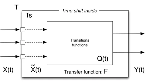
The purpose of the present work is thus to contribute to a unified formal framework for complex systems modeling & architecture. We will model the observational behavior of any real system through a functional machine pro-cessing dataflows (for related work on dataflow networks, see [37, 19, 18, 17]) in a way that can be encoded by timed transitions for changing states and outputs in instantaneous reaction to the inputs (comparable with timed Mealy machines [46]). We show that our formalization makes it possible to model all kinds of real systems (physical, software and human/organizational), which is necessary in Systems Engineering.

An underlying assumption of our approach is that each system has its own rhythm, and that this rhythm cannot be changed by an interaction with another system, nor cause sampling problems when two systems of different time scales are integrated together. This means that each system somehow has a set of characteristic predefined moments of transitions that are generally based on its internal mechanisms seen at a certain level of abstraction.

Overall, our approach towards systems modeling & architecture is simple: • we use a unified framework where continuous & discrete times are handled

5

Note thus that our purpose is not to define executable models, or an actionable formalism with a dedicated language that can be used on the field by engineers. It clearly differentiates our approach from many existing languages like Lustre[35], Simulink[68] or Altarica[7].

in a unified way

• we separate the behavior of systems that can be observed (outputs and states) and their structure (how a system is built from elementary com-ponents)

• we view all behaviors as “algorithmic”. We define and model all objects so that a system behavior can be explained as a step-by-step transformation of dataflows

• we model systems structure following a “Lego paradigm”. We explain the architecture of systems through the integration of smaller building blocks, themselves, modeled as systems

• we consider that only three actions are possible during the design process: abstracting a system, composing together a set of systems, and verifying if a system behavior respects a set of requirements6.

We generalize and extend the approach of the previous work in [12] (where a unified model for continuous and discrete systems was defined by using non-standard infinitesimal and finite time steps) by dealing with time, data, and synchronization axiomatically, and by introducing integration operators that were introduced in [30] for discrete systems only. Our purpose is to give a uni-fied and minimalist semantics for heterogeneous integrated systems and their integration. By “unified”, we mean that we propose a unified model of real systems that can describe the functional behavior of heterogeneous systems and that is closed under integration. By “minimalist” we mean that our formal-ization intends to provide a small number of concepts and operators to model the behaviors and the integration of complex industrial systems. Our work thus allows to give a relevant formal semantics to concepts and models typically used in Systems Engineering, where semi-formal modeling is well-spread.

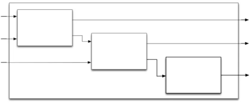
To build new systems from existing systems, we will formalize two operators that play a crucial role when modeling or designing real systems:

1. Composition operators, and 2. Abstraction operator.

Composition operators consist in building a larger system by aggregating together smaller systems and connecting together some of the inputs and outputs of those systems. As to the abstraction, it allows to define from a composition of systems a more abstract system that will itself be integrated in more global ones. In fact, abstraction aims at structuring systems at many levels of description,

6_{Requirements are used in Systems Engineering to define expected properties of systems,}

1.5. STRUCTURE OF THIS MANUSCRIPT from the most concrete to the most abstract one. The purpose of the abstraction operator is also to make easier the description of systems at more abstract levels. In this framework, integration of real systems can be modeled as a building a target multiscale system from elementary systems recursively composed and abstracted at different levels.

Based on these definitions of systems and their integration, we are able to define a minimalist systems architecture framework to deal with requirements, systems structure, and underspecification during the design process.

1.5

Structure of this manuscript

For a better understanding, this manuscript should be better read chapter af-ter chapaf-ter. Hence, we progressively build our framework. First, we define heterogeneous dataflows, and then systems as step-by-step machines transform-ing dataflows. Such systems can be integrated ustransform-ing operators, to build more complex systems, so that we can handle the two dimensions of the complexity (heterogeneity and integration). We then introduce a minimalist formalism for systems architecture to model requirements, underspecification & structure of systems through the design process. We finally open perspectives around sys-tems optimization when fairness is required.

Chapter 2, Heterogeneous dataflows, introduces formal definitions of time, data and dataflows. Our unified definition of time allows to deal uniformly with both continuous and discrete times, while our definition of data allows to handle heterogeneous data having specific behaviors. This makes it possible to define heterogeneous dataflows with generic synchronization mechanisms allowing to mix dataflows together. The deliverable is a unified and well-formalized defi-nition of heterogeneous dataflows with properties that will be later needed to define & integrate systems.

Chapter 3, Systems, defines a system as a mathematical object characterized by coupled functional and states behaviors upon a time scale. This is a definition modeling a real system as a black box with observable functional behavior and an internal state (similarly to a timed Mealy machine). This definition is ex-pressive enough to capture, at some level of abstraction, the functional behavior of any real industrial system with sequential transitions. We also express the functional behavior of systems via transfer functions transforming dataflows and show the equivalence. The deliverable is a unified definition of a system (viewed as a functional black box) and a proof of its equivalence with transfer functions. Chapter 4, Integration operators, provides formal operators to integrate such systems. Those operators make it possible to compose systems together (i.e. interconnecting inputs and outputs of various systems) and to abstract a sys-tem (i.e. change the level of description of a syssys-tem in term of granularity of all dataflows). We show that these operators are consistent with the natural

definitions of such operators on transfer functions. The deliverable is a set of integration operators that are proven to be consistent and whose expressivity allows to model systems integration. Chapters 2, 3 & 4 have been published as a journal article Complex Systems Modeling II: A minimalist and unified se-mantics for heterogeneous integrated systems [30] in Applied Mathematics and Computation (Elsevier), 2012.

Chapter 5, A logic for requirements, provides a minimalist logic to express re-quirements on systems. We first introduce an equivalent definition of systems using coalgebraic models. Based on these models, we define logical requirements to express properties on the observable behavior of systems. This chapter has been published as an article: An adequate logic for heterogeneous systems [4] at the 18th IEEE International Conference on Engineering of Complex Computer Systems (ICECCS 2013).

Chapter 6, Towards a framework for systems architecture, defines a formal framework to deal with heterogeneous integrated systems during the systems design process. Two main problems are addressed: how to deal with the un-derspecification of systems during their design process, and how to formalize the structure of a system. We consider a minimalist design process, consisting of requirements analysis and systemic recursion. We introduce the notion of views that allow to formalize the set of interrelated models used in practice to describe a more or less specified system at any step of the design process. We then introduce formal definitions of the internal structure of a system. The deliverable is a minimalist formal framework for systems architecture along the design process, with a generic framework to model underspecification and the structure of systems. This chapter has been accepted and presented at the 3rd International Workshop on Model Based Safety Assessment (IWMBSA’2013) under the title A minimalist formal framework for systems architecting [31]. Chapter 7, Fair assignments between systems, finally explores the combinato-rial optimization between subsystems, when fairness is required (for example to spread risk or cost between various units that should be assigned functions). Optimization in systems architecture is key to take design decisions during the process. Our core idea is to iterate a classical partial fairness decision criteria. The deliverable is a new, original model for fair multi-agent optimization that can be relevant to optimize design decisions during a systems design process. This chapter intends to open new perspectives and is fairly independent from the rest of the manuscript. It has been published as a paper Infinite order Lorenz dominance for fair multiagent optimization [32] at the International Conference Autonomous Agents and Multi-Agent Systems 2010.

Part I

Chapter 2

Heterogeneous dataflows

We introduce formal definitions of time, data and dataflows. Our unified defini-tion of time allows to deal uniformly with both continuous and discrete times, while our definition of data allows to handle heterogeneous data having spe-cific behaviors. This makes it possible to define heterogeneous dataflows with generic synchronization mechanisms allowing to mix dataflows together. The deliverable is a unified and well-formalized definition of heterogeneous dataflows with properties that will be later needed to define & integrate systems.

2.1

Time

Most of the challenges raised by a unified definition of complex (industrial) sys-tems are coming from time. Indeed, real syssys-tems are naturally defined according to various times, that can typically be discrete or continuous. We must therefore be able to define:

• a unified model of time encompassing continuous and discrete times to later introduce a unified definition of heterogeneous systems,

• the mixture of various time scales to integrate such systems.

Unifying both discrete and continuous times is a complicated issue (see [14] for an exhaustive survey on the subject). To reach this purpose, we propose to extend & axiomatize the approach developed in [12] where discrete and continu-ous times have been unified homogenecontinu-ously by using techniques of non-standard analysis [48, 54, 27]. We introduce a more generic approach and deal with time axiomatically, that is by expressing the minimal properties that both time refer-ences and time scales have to satisfy. That allows to consider in a same uniform framework many different times: usual ones such as N and R, or more specific ones such as the non-standard real numbers∗_{R, or the VHDL time (see below).}

2.1.1

Time reference

A time reference is a universal time in which all systems will be defined. It captures the intuition we have of time: a linear quantity composed of ordered moments, pairs of which define durations. Such a modeling of “time” will be common to all the systems we want to integrate together.

Definition 2.1.1 (Time reference) A time reference is an infinite set T together with an internal law +T _{: T × T → T and a pointed subset (T}+_{, 0}T₎

satisfying the following conditions: • upon T+:

– ∀a, b ∈ T+, a +T b ∈ T+ closure (∆1)

– ∀a, b ∈ T+_{, a +}T _{b = 0}T _{=⇒ a = 0}T _{∧ b = 0}T _{initiality (∆} 2)

– ∀a ∈ T+, 0T +T a = a left neutrality (∆3)

• upon T :

– ∀a, b, c ∈ T, a +T _{(b +}T _{c) = (a +}T _{b) +}T _{c associativity (∆} 4)

– ∀a ∈ T, a +T ₀T _{= a right neutrality (∆} 5)

– ∀a, b, c ∈ T, a +T _{b = a +}T _{c =⇒ b = c left cancellation (∆} 6)

– ∀a, b ∈ T, ∃c ∈ T+_{, (a +}T _{c = b) ∨ (b +}T _{c = a) linearity (∆} 7)

Elements of T are moments whilst elements of T+ _{are durations (i.e.}

dis-tances between moments). Any duration can be considered as a moment, by setting a conventional origin.

The properties given upon T and T+ _{are constraints that catch the intuitive}

view that the time elapses linearly by adding successively durations between them.

Proposition 1 (Total order on a time reference) We can define a total order )T _{(later written ) for convenience) on T as follows:}

a )T b ⇔ ∃c ∈ T+, b = a +T c

Proof This is a classical result using ∆2, ∆4, ∆5, ∆6 and ∆7 (time references

are similar to specific semigroups, cf [24]). )T _{is reflexive by ∆}

5, transitive by ∆4, total by ∆7. To be a total order,

it should moreover be antisymmetric. Suppose that a )T b and b )T a. Thus, ∃c, d ∈ T+ _{such that b = a +}T_{c and a = b +}T _{d. But then: a = b +}T _{d = (a +}T

c)+T_{d = a+}T_(c+T_{d) by associativity ∆}

4. But by ∆5, a+T0 = a = a+T(c+Td),

and so by ∆6, c +T d = 0T. As c, d ∈ T+, we have by ∆2 that c = d = 0T and

finally by ∆5 again a = b. )T is antisymmetric and is therefore a total order.

2.1. TIME Moreover, we can remark that ∆1 ensures that any element of T greater

than an element of T+ _{will be in T}+_{, and ∆}

3 ensures that 0T is the minimum

of T+_{, so that the set of durations has natural properties according to )}T _and

can be understood as “positive” elements of T .

Example 1 In [12], the time reference is the set of non-standard real numbers

∗_{R defined as the quotient of real numbers R under the equivalence relation}

≡⊆ RN

× RN

defined by:

(an)n≥0≡ (bn)n≥0 ⇐⇒ m({n ∈ N|an= bn}) = 1

where m is an additive measure that separates between each subset of N and its complement, one and only one of these two sets being always of measure 1, and such that finite subsets are always of measure 0. The obvious zero element of

∗_{R is (0)}

n≥0, ∗R+ is its positive part taken here as durations, and the internal

law + is defined as the usual addition on RN

, i.e.: (an)n≥0+ (bn)n≥0= (an+ bn)n≥0

∗_{R satisfies all the conditions of Definition 2.1.1 and is a well-defined time}

reference. Observe also that∗_{Rhas as subset, the set of non-standard integers}∗_Z

(and subsequently ∗N_{) where infinite numbers are all numbers having absolute}

value greater that any n ∈ N. ♦

Some authors, e.g. [38], add commutativity and Archimedean properties in the definition of a time reference. Commutativity is intuitive and the Archimede-an property excludes Zeno’s paradox. However, they are not always satisfied by standard models of time, as in the VHDL time used in some programming languages.

Example 2 The VHDL time [13] V is given by a pair of natural numbers (both sets of moments and durations are similar): the first number denotes the “real” time, the second number denotes the step number in the sequence of compu-tations that must be performed at the same time – but still in a causal order. Such steps are called “δ-steps” in VHDL (and “micro-steps” in StateCharts). The idea is that when simulating a circuit, all independent processes must be simulated sequentially by the simulator. However, the real time (the time of the hardware) must not take these steps into account. Thus, two events e1, e2

at moments (a, 1), (a, 2) respectively will be performed sequentially (e1 before

e2) but at a same real time a. The VHDL addition is defined by the following

rules:

(r′ .= 0) =⇒ (r, d) + (r′, d′) = (r + r′, d′) (r′= 0) =⇒ (r, d) + (r′, d′) = (r, d + d′)

where r, r′, d and d′ are natural numbers and + denotes the usual addition on natural numbers. Clearly, the internal law + above is not commutative,

nor Archimedean: we may infinitely follow a δ-branch by successively adding

δ-times.1 _♦

2.1.2

Time scale

Time references give the basic expected properties of the set of all moments. Now, we want to define time scales, i.e. sets of moments of a time reference that will be used to define a system (systems can indeed have various paces & origin dates).

A time scale will later be used to define step-by-step behavior of system, which makes it necessary to define it as a sequence of moments.

Definition 2.1.2 (Time scale) A time scale is any subset T of a time ref-erence T such that:

• T has a minimum mT

∈ T

• ∀t ∈ T, T_t+= {t′_{∈ T | t ≺ t}′_{} has a minimum called succ}T

(t) • ∀t ∈ T , when mT

≺ t, the set Tt− = {t′ ∈ T | t′ ≺ t} has a maximum

called predT

(t)

• the principle of induction2 _{is true on T.}

The set of all time scales on T is noted T s(T ).

A time scale is defined so that it will be possible to make recursive con-structions on it, and to locate any moment of the time reference between two moments of a time scale. A time scale necessarily has an infinite number of moments. In fact, a time scale is expected to comply with the Peano axioms3_,

excepted that the succT

and predT

are defined for moments of T and not only T_.4

This is not equivalent: a simple counter-example on time reference R+can show it is possible to have pred and succ properly defined for moments of the subset T = {1 −₂1nfor n ∈ N} ∪ {1 + 1

2nfor n ∈ N} whereas moment 1 has no pred or

succ in T . This fundamental property prevents Zeno’s effect on any time scale. Most of time scales (discrete and continuous) used when modeling real sys-tems can be defined as unified regular time scales of step τ and of minimum m:

m m + τ m + 2τ m + 3τ ...

1_{This is not the intended use of VHDL time, however: VHDL computations should perform}

a finite number of δ-steps.

2

For A ⊂ T,!mT

∈A& ∀t ∈ A, succT_{(t) ∈ A" ⇒ A = T.}

3_{It can be easily checked that the above conditions imply Peano axioms.}

4_{These specific properties will be necessary to prove that time scales are closed under finite}

2.1. TIME Example 3 By using results of non-standard analysis, continuous time scales can then be considered in a discrete way. Following the approach developed in [12] to model continuous time by non-standard real numbers, a regular time scale can be ∗Nτ where τ ∈ ∗R+ _{is the step, 0 ∈} ∗Nτ and ∀t ∈ ∗Nτ, succ∗N_τ

(t) = t + τ . This provides a discrete time scale for modeling classical discrete time (when the step is not infinitesimal) and continuous time (when

the step is infinitesimal). ♦

Example 4 In the VHDL time V, the internal law induces a lexicographic ordering on N × N. Thus, let W ⊂ V such that: ∀a ∈ N, ∃Na ∈ N, ∀(a, b) ∈

W, b ≤ N_a (i.e. there are only a finite number of steps at each moment of time in W). Then W is a time scale in the VHDL time. ♦ Example 5 A time scale on the time reference R+ _{can be any subset A such}

that: ∀t, t′∈ R+, |A ∩ [t; t + t′]| is finite. ♦ We have shown that we can accommodate heterogeneous times with our definitions. We introduce a fundamental proposition allowing to unify different time scales, which will be necessary for systems integration (when the systems involved do not share the same time scales). Overall, our definition of time will be suitable for heterogeneous integrated systems.

Proposition 2 (Union of time scales) A finite union of time scales (on the same time reference T ) is still a time scale.

Proof The proof for two time scales is enough.

Let T1, T2 be two time scales on T . Let T = T1 ∪ T2. We want to prove

that T is a time scale.

Tis a subset of T . Note that T has a minimum min!mT₁

, mT_{2", and that ∀t ∈ T ,}

the succ and pred functions can be obviously defined by: • succT (t) = min!succT₁ (t), succT₂ (t)" • when t 5 mT , predT = max!predT₁ (t), predT₂ (t)"₅

We need to prove that the induction principle holds on T. This can be proved by using a lemma: if mT

∈ A & ∀t ∈ A, succT

(t) ∈ A then ∀t ∈ Ti, t ∈ A ⇒

succTi_{(t) ∈ A for i = 1, 2. This lemma is proved using the principle of induction}

in Ti on intervals of successive elements of Ti in T:

Let P (t) be a proposition such that: ∀t ∈ T, P (t) ⇒ P!succT

(t)" (L0). We want to show that: ∀t ∈ T1, P (t) ⇒ P!succT1(t)

"

(L1). Let t ∈ T1 and

t′ = succT₁

(t). If t′ = succT

(t), then (L1) is true for this t by (L0). Else: let ta = succT(t) and tb = predT(t′). Then ta, tb ∈ T2 and succT (by construction

5_{for convenience of writing, we assume that if pred}Ti _{is not well defined for its argument,}

its value is mT

equals to succT₂

since there is no moment of T1 between ta and tb) defines, by

induction in T₂, a set of successive elements of T₂ between t_a and t_b. If P (t) is true, then P (ta) is true by (L0).

The principle of induction which is true in T2can be applied to the set [ta, tb]

of moments of T1, so that P (tb) is true, and finally P (t′) = P!succT(tb)" is true

by (L0).

What means that P (t′) = P!succT₁

(t)"

is true. Finally, we have shown that: (L0) ⇒ (L1). We can show the same property (L’1) on T2. Applying

independently the principle of induction for proposition P on T1and on T2, we

have that: if P (mT

) is true, P is true on T1and P is true on T2. The

proposi-tion P is true on their union T. Therefore, the principle of inducproposi-tion is true on T. Finally, T = T1∪ T2 satisfies the principle of induction, and thus T is a time

scale on T . !

Remark 1 It is easy to show that the union of an infinite number of time scales can define a set of moments that is not a time scale. We recall the example T = {1 − 1

2nfor n ∈ N} ∪ {1 + 1

2nfor n ∈ N} where moment 1 has no pred or succ in T . Let define an infinite sequence of time scales: ∀n ∈ N, Tn =

{1 − ₂1n} ∪ {1 + 1

2n} ∪ N. The union T =

#

n∈N

T_{n is not a time scale since the} moment 1 has no pred or succ in T.

In our approach of time, even if the time reference is for instance R, we do not set a discrete time reference, so that although all time scales on R are discrete and isomorphic to N, they are not constrained by a predefined universal discrete time. Thus, our approach allows to define finer time scales for modeling real systems (which can work at different rhythms or with shifts of phase) than considering a given discrete time reference (as done for instance with reactive systems [43], where a universal sequential clock sets a given granularity that cannot be further refined6).

2.2

Data

Another challenge to address to model complex systems is the heterogeneity of data (modeling any element that can be exchanged between real systems) and of their synchronization between different time scales. We introduce datasets that will be used for defining data carried by dataflows.

2.2.1

Datasets

Definition 2.2.1 (#-alphabet) A set D is an #-alphabet if # ∈ D. For any set B, we can define an #-alphabet by B = B ∪ {#}.

6

2.2. DATA The elements of an #-alphabet are called data and # is a universal blank symbol # accounting for the absence of data (as the blank symbol in a Turing machine)7_.

An #-alphabet can have an infinite number of data. A system dataset (also called dataset) is an #-alphabet with the description of the behavior of the data: Definition 2.2.2 (System dataset) A system dataset is a pair D = (D, B) such that:

• D is an #-alphabet

• B, called data behavior, is a pair (r, w) with r : D → D and w : D ×D → D such that8_: − r(#) = # (R1) − r!r(d)" = r(d) (R2) − r!w(d, d′_{)" = r(d}′_{) (R3)} − w!r(d′_{), d" = d (W 1)} − w!w(d, d′_{), r(d}′_{)" = w(d, d}′_{) (W 2)}

Remark 2 We will sometimes use interchangeably the #-alphabet and the dataset in our definitions & examples if it is more convenient and when there is no am-biguity.

B will be useful to synchronize dataflows defined on different time scales (see Projection below). Data behaviors can be understood as the functions allowing to read and write data in a “virtual” 1-slot9 _{buffer defining how this}

synchro-nization occurs at each moment of time:

• when a buffer is read, what is left (depending on the nature of data, it can partially vanish)

• when a new data is written (second parameter of w), knowing the current content of the buffer (first parameter of w), what is the new content of the buffer (depending on the nature of data and the new incoming data, it can be partially or totally modified).

In this context, the conditions on r and w can be understood as follows: • (R1): reading an empty buffer (i.e. containing #) results in an empty

buffer

• (R2): reading the buffer once or many times results in the same content of the buffer

7_{basically, introducing this blank means that a flow “transmitting nothing” at a given}

moment will be coded as a flow transmitting " at this moment.

8_{These axioms give a relevant semantics and are necessary to define consistent projections}

of dataflows on time scales.

9

1-slot means that the buffer can contain only one data. This data will be used to compute the value of a dataflow at any moment of a time scale, to be able to synchronize a dataflow with any possible time scale.

• (R3): reading a buffer in which a data has just been written results in the same content whatever the initial content of the buffer was before writing the data

• (W1): when the buffer has just been read, the new data erases the previous one

• (W2): when the buffer has just been written with a data, it will not be modified if it is again written with the result of the reading function on this same data10

• we also have by (R1) + (W1): w(#, d) = d (W3). When an empty buffer is written with a new data, the buffer contains this new data.

2.2.2

Implementation of standard data behaviors

There are two classical examples of data behaviors when modeling real systems: Example 6 [Persistent data behavior] In this case, data cannot be con-sumed by a reading, and every writing erases the previous data (this data be-havior was the only one used in [12]):

r(d) = d and w( , d) = d

♦ Example 7 [Consumable data behavior] In this case, data is consumed by a reading, and every writing (excepted when it is #) erases the previous data:

r(d) = # and w(d, d′) = $

d if d′= # d′ else

♦ We give a less classical example of data behavior that can be used to rep-resent the ability to accumulate data received (what can be meaningful when data are written more frequently than read). It is important to notice that the buffer is still a 1-slot buffer and that all accumulated data will be consumed entirely by a single reading11_.

Example 8 [Accumulative data behavior] Let A be a non-empty set and D = P(A) be the set of subsets of A. We consider that # = ∅, so that D is an

10_{This rule will ensure that a dataflow projected on a finer time scale is equivalent to the}

initial dataflow.

11

Modeling another kind of reading shall be modeled by buffers in the system itself, this is not the purpose of these “virtual” buffers dedicated to synchronization of data between different time scales.

2.3. DATAFLOWS #-alphabet12. In this case, data is consumed by a reading, and every writing is added (using internal law of D, here ∪) to the previous data:

r(d) = # and w(d, d′) = d ∪ d′

♦ It is straightforward to check that these examples are compliant with the axioms of data behaviors.

Remark 3 The same real data can be modeled using different behaviors: for instance, an electric current might be measured by a number of electrons at each step of a time scale (consumable behavior, data expressed as a natural number), or by a continuous flow of electrons (persistent behavior, data expressed as a real number in Amperes). Thus, a data behavior is not an intrinsic property of the real data it models, but a modeling choice.

2.3

Dataflows

The dataflows will be used to describe variables of systems (inputs, outputs and states). We also define the synchronization of dataflows between time scales (to be able to properly define the integration of systems with different time scales).

2.3.1

Definition

In what follows, D will stand for a dataset of #-alphabet D with behaviors (rD, wD). A dataflow is a flow defined at the moments of a time scale carrying

data of a dataset. It will be used to define the evolution of states, inputs and outputs of a system.

Definition 2.3.1 (Dataflow) Let T be a time scale. A dataflow over (D,T) is a mapping X : T → D.

Definition 2.3.2 (Sets of dataflows) The set of all dataflows over (D,T) is noted DT

. The set of all dataflows over D with any possible time scale on time reference T is noted DT ₌ #

T_{∈T s(T )}

DT

.

2.3.2

Operators

We introduce an operator making it possible to project a dataflow on any time scale. The mechanism to compute the resulting dataflow correspond to the idea that there is an intermediary buffer which stores or outputs the values of the initial dataflow so that they can be read according to the new time scale. The projection of a dataflow on a time scale makes it possible to synchronize a

12

dataflow between two different time scales, with the rule that a data arriving at t will be read at the first next moment on the time scale of projection (the computation of this synchronization only requires a 1-slot virtual buffer and data behaviors). It will be essential when composing together systems using different time scales to define the properties of the exchange of data.

Definition 2.3.3 (Projection of a dataflow on a time scale) Let X be a dataflow over (D, TX) and TP be a time scale. Let T = TX ∪ TP. Let T′P =

succT

(TP)13. We define recursively the buffer function b : T → D by 14:

• (P1) if t ∈ TX \ T′P, b(t) = w!b(pred T (t)), X(t)" • (P2) if t ∈ T′_P \ TX, b(t) = r!b(predT(t)) " • (P3) if t ∈ TX ∩ T′P, b(t) = X(t) • (P4) if t ∈ TP \ (TX∪ T′P), b(t) = b(pred T (t))

The projection XTP of X on TP is then the dataflow over (D, TP) defined by setting XTP(t) = b(t) for every t ∈ TP.

T

T

The semantics of each part of the definition is the following: (P1) occurs when a new data is received, and when the data on the buffer has not been read at the previous step so does not need to be processed with the reading function. (P2) occurs when no new data is received, and when the data on the buffer has been read at the previous step and so needs to be processed in the buffer with the reading function. (P3) occurs when a new data is received, and when the data on the buffer has been read at the previous step, so that the content of the buffer is the new data, by condition (W1). Finally, (P4) occurs when no new data is received, and when the data on the buffer has not yet been read, so that nothing changes.

Remark 4 It is straightforward to show that the projection of a dataflow on its own time scale does not alter the dataflow (as only P3 occurs): XTX = X

We define equivalent dataflows as dataflows that cannot be distinguished by any projection. It is useful to be able to compare data flows defined on different time scales (but that will have exactly the same behavior for any given system).

13_{Corresponding to moments such that a data has been read at the previous moment and}

shall be marked as “read”.

14_{By convention, b!pred}T_(mT_{)" = ", which makes it simpler to define the rules of projection}

without making a special case when t = mT

2.3. DATAFLOWS Definition 2.3.4 (Equivalent dataflows) Two dataflows X and Y are equiv-alent (noted X ∼ Y ) if, and only if:

for any time scale T on T, XT= YT

Example 9 Let X be a dataflow over (D, T) where D as a persistent data behavior and T is a regular time scale of step τ and minimum m. Let T′ be the regular time scale of step τ /2 and minimum m. Let X′ _{be the dataflow over}

(D, T′_{) defined by: ∀t ∈ T, X}′_{(t) = X}′_{(t + τ ) = X(t). Then, X ∼ X}′_{. The}

intuition behind this result is that X′has 2 moments for each moment of X but carry the same persistent data, so that they cannot be distinguished.

Definition 2.3.5 (Equivalent dataflows as far as) Two dataflows X and Y are equivalent as far as t0∈ T (noted X ∼t0 Y ) if, and only if:

for any time scale T on T, for all t ) t0 in T, XT(t) = YT(t)

2.3.3

Consistency of dataflows

We introduce two propositions insuring the consistency of our definition of dataflows. These propositions will be useful to prove the consistency of op-erators we define in Chapter 4. The first proposition ensures that the way we define the projection of a data flow on a finer time scale is consistent with the equivalence relationship we have naturally defined on dataflows:

Proposition 3 (Equivalence of projection on a finer time scale) Let X be a dataflow on (D, TX) and let TP be a time scale such that TX ⊆ TP. Then,

we have:

X ∼ XTP

Proof The proof uses the properties of the data behaviors and the principle of induction on time scales to show that: ∀T ∈ T s(T ), XT = (XTP)T, and thus

X ∼ XTP (by definition of ∼). Let T be a time scale. We note P = XTP and

want to prove that XT= PT.

Let bX be the buffer (defined for moments of TX∪ T) used for defining the

projection of X on T and bP be the buffer (defined for moments of TP∪ T) used

for defining the projection of P on T. We will prove by induction on T that: ∀t ∈ T, bX(t) = bP(t).

(a) First, we want to prove that the equality is true for moments before mTX_.

Let t0 ∈ T with t0 ≺ mTX (we will suppose without loss of generality15 that

mT

≺ mTX_).

• XT(m T

) = # by (P0) + (P4) to initialize the buffer. • for P :

15

– if mT

≺ mTP_{, then P}

T(mT) = # by (P0) and (P4)

– else: we have ∀t ∈ TP | t ≺ mTX, P (t) = XTP(t) = # by (P0) and

(P4) since mT

≺ mTX_{. As w(#, #) = # by (W3) and r(#) = # by (R1),}

the buffer till mT

in the projection of P on T is alway equal to # and we have PT(mT) = #. • finally, XT(m T ) = PT(m T ).

• we can extend the proof by induction to any t0 ∈ T with t0≺ mTX since

∀t ∈ TP such that t ≺ mTX, P (t) = #.

(b) For the case where t = mTX_{, we have b}

X(t) = bP(t) = X(mTX), which will

allow to initiate the induction.

(c) Then, we want to prove that the induction hypothesis can be used on T. Let t0∈ T with t0 8 mTX such that bX(t0) = bP(t0) and t1 = succT(t0). We want

to prove that bX(t1) = bP(t1). Let A =]t0; t1] ∩ TP 16 and B =]t0; t1] ∩ TX (we

have B ⊆ A since TX ⊆ TP). Let tx = predTX!succTX(t0)

"₁₇

. Three cases are to be considered: • (1.1) if B = ∅ and A = ∅ – for bX(t1): by (P2) we have bX(t1) = r!bX(t0) " – for bP(t1): by (P2) we have bP(t1) = r!bP(t0)" = r!bX(t0)" – and so bX(t1) = bP(t1).

• (1.2) if B = ∅ and A .= ∅, two subscases shall be considered – (1.2.1) if tx = t0, then

∗ for bX(t1): by (P2) we have bX(t1) = r!bX(t0)". According to

the situation: by (P3) bX(t0) = X(t0) = w!#, X(t0)" or by (P1)

bX(t0) = w! . . . , X(t0)". Anyway, bX(t0) = w! . . . , X(t0)", and

by (R3) we have bX(t1) = r!X(t0)".

∗ for bP(t1): ∀t ∈ A, P (t) = r!X(t0)", using (P2) and (R2) in

the definition of P as the projection of X on TP. So, by (P1)

we have bP(mA) = P (mA) = r!X(t0)". As w!r(d′), d" = d by

(W1), we have applying (P1) for all t ∈ A, bP(t) = r!X(t0)".

If t1 ∈ A, we apply (P4) and get: b/ P(t1) = r!X(t0)", and the

result is the same if t ∈ A. ∗ and so bX(t1) = bP(t1).

– (1.2.2) if tx ≺ t0, then

16_{This notation is intended to capture the elements of T}

P greater than t0 and less than or

equal to t1. 17