Information to share in supply chains dedicated to the mass production of customized products for decentralized management

Laboratoire d'Analyse et Modélisation de Systèmes pour l'Aide à la Décision CNRS FRE 3234

CAHIER DU LAMSADE

302

janvier 2011

Information to share in supply chains dedicated to

the mass production of customized products for

decentralized management

Information to share in supply chains dedicated to the mass production of

customized products for decentralized management

C. Camisullis1, V. Giard2, and G. Mendy-Bilek3

1 _{IRG, Université Paris-Est– France (carole.camisullis@univ-paris12.fr)} 2 _{Université Paris-Dauphine – France (vincent.giard@dauphine.fr)} 3

IAE, Université de Pau et des Pays de l’Adour – France (gisele.mendy-bilek@univ-pau.fr)

Abstract

In an upstream supply chain dedicated to the mass production of customized products, decentralized management can be an efficient and effective method in a steady state in which stochastic characteristics of customers’ demands remain stable. However, this is possible only if all echelons that precede the final assembly line use periodic replenishment policies that restrain the stockout risk to a low predetermined probability. The safety stocks’ levels are more difficult to define for alternative or optional parts, as well as the components they use, whose demands are weighted sums of random variables, affected by several random factors and organizational constraints. The factors and constraints to consider are not the same for supplied and produced components. The random demand of a component depends on the demand of alternative or optional parts mounted in the final product, through a double transformation involving the bill of materials explosion, which is at the origin of the weighted sum of random variables, and time lags. In the steady state, the knowledge of the probability distribution of that random variable allows for the determination of safety stocks that decouple the management of upstream supply chains. Progressive changes in the steady state require periodic and progressive adaptations of the safety stocks that do not directly depend on the final demand knowledge.

Keywords: supply chain coordination, information sharing, upstream supply chain, bullwhip effect,

periodic review policy, order penetration point

1. Introduction

In mass production systems of customized products that use a build-to-order supply chain (BTO-SC; Anderson and Pine, 1997; Gunasekarana and Ngaib, 2005, 2009), differentiation results from the combination of n optional or alternative components. These components come from n different sets and are assembled on n different workstations in an assembly line. The upstream supply chain (USC) thus consists of units that contribute to the production of the final assembly line. The various links of the chain connect through flows of products and information. In addition, production decisions made by the last production link (i.e., the assembly line) determine the production of the USC.

Two obstacles prevent centralized control of the USC by assembly lines: Many units belong to independent companies, and a link might belong to several supply chains (e.g., supply chains

monitored by Ford and General Motors have many common links). The behavior of the chain, and thus its global performance, depends on the information and product exchanges that take place among the links, as well as the control rules used to make provisioning and production decisions.

The BTO-SC is characterized by slow changes in the level and structure of final demand. In this context, USC echelons may use periodic policies, with rules that assume steady state and are periodically revised, ensuring decision autonomy and avoiding the propagation of disturbances. This independence implies safety stocks with properly defined levels to guarantee against a given stockout risk (effectiveness) at the lowest cost (efficiency). This article examines provisioning and production decisions in a BTO-SC that deals with optional or alternative components and the various parts those components require. We combine results from supply chain literature to suggest efficient rules for monitoring the provisioning or production of optional or alternative parts and their components. Not only is this global scope relatively new, but in comparison with existing literature, our approach offers three key specificities as well.

Prior research suggests several reasons to maintain safety stock in a supply chain, namely, to mitigate stockout risks due to random variations of demand, delivery lead times, quality problems, or forecast errors, which also determine the necessary risk to account for in supply or production orders. Hundreds of analytical models combine different hypotheses regarding demand characteristics and behavior, pricing, provisioning, and physical or financial constraints; in general, they produce expected cost functions and offer analytical solutions based on optimal stockout probabilities that depend on the cost structure. Simulation models can often find good solutions when models are too complex to yield analytical solutions. However, for the type of USC we study, the costs a stockout induces, which triggers the stoppage of assembly lines, are so high that the use of an analytical model based on some expected cost function is ineffective. Instead, we suggest basing the provisioning policy of optional or alternative parts (and their components) on periodic replenishment rules that depend on an arbitrary, very low stockout probability; the order-up-to level defines the safety stock. The demand of an optional or alternative part (or one of its components) is a weighted sum of random variables due to the bill of materials (BOM) explosion and is affected by a combination of several random factors (e.g., probability of use, variable lead time, quality problems) and logistics constraints (batch size, transport capacity limitation) or organizational constraints. Determination of an optional or alternative part is tractable through the use of the Monte Carlo approach.

In addition, the pernicious effects of decisions based on local information are well known for the downstream supply chain, especially for low-cost, standardized, mass products. They propagate oscillations of increasing amplitude along the supply chain (Forrester, 1958), creating the bullwhip effect (BWE; Lee et al., 2004). Several causes of the BWE are listed in Lee et al.’s (1997) classic article and extended in other articles, and Gearya et al. (2006) point out the main issues of the BWE. Several articles have tried to quantify the BWE, though rarely in the real world (Hanssens, 1998) and usually in a hypothetical context (Ouyang and Li, 2010; Springer and Kim, 2010). In general, the

supply chain is limited to a set of two linked nodes or sometimes to a serial network; several articles also discuss a general network (Ouyang and Li, 2010; Sucky, 2009) but then rarely extend it to the first-tier suppliers of assembly lines (plant level) or further, even in macro-economic studies (Cachon, 2007). In most cases, research solely considers supply chain distribution, focusing on the mass production of customized products. Furthermore, prior research relies on two main modeling approaches—analytical (e.g., Lee et al., 1997) and simulation (e.g., Sucky, 2009)—to suggest solutions to mitigate the BWE, generally through information sharing. In contrast, we consider the USC from a general network perspective, using an analytical approach; we are not interested in measuring the BWE or suggesting solutions to avoid it. In the context of the automotive industry, which we study, BWE is observable, but its mechanisms are relatively unknown. Because of their high selling prices, cars are subject to individual tracking; thus, the amplification effects observed in the distribution networks of low-cost, mass products are unlikely to occur. Upstream, production aims to meet the demands of a single customer, the final assembly line. Without reliable information, autonomous USC plants are likely to overreact to stock shortages and the presence of excessive inventories, which should yield increasing fluctuations along the USC even as the daily production of the final assembly line remains stable. Therefore, the daily consumption of optional or alternative components varies, but their randomness may be poorly estimated in provisioning decisions. Even commercial actions (e.g., rebates, incentives, limited series) by the company that owns the final assembly line can generate disturbances along the USC. We show why the transmission of appropriate information to each echelon enables the avoidance of BWE, if properly used, and allows decentralized management.

Finally, information sharing is the last point we use to position our article. Firms can share raw information, such as sales histories, orders, inventory positions, and deliveries, or they can share processed information related to planned or forecast demand (Ryu et al., 2009). Different forms of information sharing are useful for decreasing costs and risks in short-term decision making (Chandra

et al., 2007). The propagation of demand also means that many companies can improve the

performance of their supply chain by treating the value of information as an important issue. Most research classifies the shared information problems according to the structure of the supply chain, the decision level, the production information model, and the improvement of a supply chain’s performance.

Accordingly, most articles focus on sharing information in a two-level supply chain structure— that is, between producers and distributers—to improve order preparation through an automatic reduction of costs and a decrease of stock-out. This configuration ignores the problem of capacity allocation and the phenomenon of shared resources. Regarding the production information model, various approaches note that a system can use a build-to-stock strategy in a traditional supply chain, but this literature still leaves gaps regarding the repercussions for a BTO-SC if the value of information pertains strongly to the positioning of the order penetration point (OPP) or if the products

in the USC are not the same. Sharing information and coordinating flows make it possible to improve the performance of a supply chain, as well as the source, nature, potential, and localization of information—topics that remain vague in existing literature. For example, Cachon and Fisher (2000) claim that the operational benefit of sharing information and coordination can span from 0% to 35% of the total costs. This disparity relates to the various structures of the chain, assuming that operations vary from one chain to another, and the problems considered. Most research focuses on a build-to-stock strategy and assumes stationary and stochastic demand, as well as an infinite planning horizon. Cachon and Fisher (2000) also study the value of information in a supply chain with one supplier, N identical retailers, and independent and identically distributed demands. With a moving average demand forecast method, Chen et al. (2000) reduce the BWE by centralizing the demand information. In modeling the value of information sharing, most studies assume that the supplier has full knowledge of the underlying demand model and the order policy used by the retailer, an unrealistic assumption for a BTO-SC. As we show subsequently, for the USC, the shared information is not raw data but rather the result of a double transformation.

We begin by investigating a steady state of periodic provisioning policies in the supply chain and then considering the conditions in which it is possible to use information to adapt steady-state policies, preserve their performance, and detect the transformations of the demand structure. Because ignoring such rules may disturb the functioning of the USC, decentralized management in the supply chain requires information sharing and the use of consistent management rules across various links.

In Section 2, we define those rules in the steady state, for alternative or optional components and their parts, taking into account the randomness of exogenous factors and the incidence of organizational parameters. In Section 3, we discuss adaptation of those rules when the steady-state assumptions do not hold. Some disturbances in the BTO-SC are generated as a result of decisions made by the company that owns the final assembly line; thus, we explain why information to define the correct provisioning or production rules for a given echelon of the USC is not raw data about final demand but rather a result of a double transformation. We also provide solutions to some implementation problems. In the conclusion section, we emphasize that specific information sharing in a BTO-SC, which guarantees decision autonomy and performance, requires effective cooperation across USC echelons.

2. Conditions of decision independence of USC units in a steady state

In the steady state, daily production by the BTO-SC is constant, and the structure of demand is stable. In this context, periodic policies can monitor production and supply at each stage of the USC. Appropriate safety stocks guarantee the independence of decisions in these stages. A general analysis of USC safety stocks shows some shared characteristics and the need to distinguish safety stocks of supplied components from those of produced components.

2.1. General analysis of safety stock needs in the steady state

First, we introduce reasons to create safety stocks. Second, we consider the characteristics of the distribution to calibrate the safety stock and specify the factors that influence it. Third, we reveal the relationship between safety stocks and stockout probability. Fourth, we study the analytical relationship between safety stocks and expected stock before delivery. The appendix presents a summary of notations used.

2.1.1. Location and justification for safety stocks

A replenishment policy includes safety stocks to address unknown demand. The stock might include products ordered to meet the needs of a production (or distribution) unit, as well as those manufactured by a production unit when that unit cannot build to order completely. A basic periodic replenishment policy places a periodic order equal to the difference between its order-up-to level R and the inventory position observed at the time of the order. The order interval is θ, and R depends on the target stockout probability α before the delivery, which might be given by economic calculations. Safety stock equals the difference between R and the average demand over the same period. Safety stock also appears in replenishment policies of the type “order quantity q – reorder point r,” in which

r behaves like R. High value of α can lead to negative safety stock, which is meaningless from an

operational point of view.

In periodic replenishment policies, the safety stock definition depends on the order-up-to level R. Inventory models use cost functions to propose analytical optimal relations to determine R, which always corresponds to the percentile of the demand distribution associated with an optimal value of the stockout probability α, which in turn depends on the cost structure in the cost function. In general, for members of the USC, unsatisfied demand is delayed, and α is very low. In that case, two observations emerge: For the supplier, the ordered quantity, which corresponds to a sum of random demand, is a random variable that reflects the demands its customer must satisfy. This property is not valid if some supplied parts are rejected for quality reasons; it is then necessary to add the number of rejected components to demandsince the last order.

With a relevant calibrationof safety stock in the various stages, a supply chain can operate without significant fluctuations. The quality of the calibration mainly depends on the propagation of appropriate information from downstream to upstream. We analyze the safety stocks of stage B in the sub-network A → B → C in a supply chain. Stage B might hold two kinds of safety stocks because of its upstream and downstream relationships.

First, production safety stocks include the components i produced by B to be sold to its customer (stage C) when the OPP of C in its production system does not allow B to build to order completely. These safety stocks are held by the supplier. We assume that customer C transmits an order of qit

components i to its supplier B at the beginning of day t. The delivery occurs at the beginning of day

iL

R _α, and the lead time is λi (λ ≤_i D_i). The next order is placed at the beginning of day t+θ_i, after

which supplier B has D_i−λ_i days to fulfill the order. If this duration is lower than the manufacturing lead time Fi of component i, the supplier fills the order by taking the needed quantities from its stocks.

The process depends on both the random characteristics of customer demand and the accepted stockout risk. In the opposite case (D_i−λ_i>F_i), B can build to order. If the interval D_i−λ_i is greater than the order interval θ_i, C uses the information from its production schedule beyond its immediate needs. The anticipation of a requirement enables B to move from a build-to-stock to a build-to-order production system. Furthermore, it allows supplier A, producing for B, to build to order. This propagation increases effectiveness (fewer stockouts) and efficiency (less safety stock) at the same time. However, this assertion cannot hold if product quality is not guaranteed.

Second, provisioning safety stocks relate to component j acquired from a supplier (A) to be used in production by B. These stocks are held by the customer (here, B), in contrast with the preceding case. The order qjt of the component j sent by B to its supplier A at the beginning of day t is delivered at the

beginning of day t+Dj with a delivery lead time λj (λj≤Dj). When B sends A an order, B has

already defined the production program for using component j up until the beginning of day t+Pj. If

the planning horizon Pj is higher than or equal to the due date time Dj, the order corresponds exactly

to the forecast consumption, and no safety stock should be held. Otherwise, if (D_j >P_j), safety stock is necessary if the order is based entirely on statistical knowledge of needs (D_j−P_j ≥θ_j) or if it relies partly on firm demand and partly on statistical knowledge of needs during the period (

j

j j

D −P <θ ). Several factors combine to influence the determination of the probability distribution of demand for one period. It requires the use of a Monte Carlo simulation to calculate the distribution empirically. An alternative component i always has the same probability pi of being included in a

product. Therefore, demand for that component is a random variable that comprises three sources of variation: (1) the size of the production set to consider, or the product of daily production n by the number L of production days, where L can be certain or random (a priori, L can be random only for the supplier’s components); (2) in the steady state, where the demand to satisfy XiL is defined for L days,

which follows a binomial distribution B(nL, pi); and (3) if a delivered product has a positive probability πi of being defective, XiL demand has little chance of being satisfied entirely, so the distribution must

include the quality impact. Therefore, we consider four elementary cases.

Case 1 (constant number L of days of demand to cover, guaranteed quality). The binomial

distribution is not continuous, nor is its cumulative distribution. The definition of a percentile RiLα

implies a convention: We retain the lowest value of RiLα, such that demand XiL has a probability lower

Case 2. If L is random and quality is guaranteed, demand XiL follows a binomial distribution

B (nL, pi). The number of trials is a random variable, so the determination of this probability

distribution is analytically complex. It can be achieved empirically with the Monte Carlo method. If L is discrete, these distributions present a multimodal pattern that becomes more accentuated as the probability pi increases.

Cases 3 and 4. L is deterministic or random, but quality is not guaranteed, so a delivered

component is defective with probability πi. To meet XiL demand, it is necessary to obtain an extra

quantity ziL and make XiL + ziL components available. The number of defective parts in this case

follows the binomial distribution B (XiL + ziL, πi). The ziL quantity is an occurrence of the random

variable ZiL, which follows the negative binomial distribution NB (XiL, πi), whose cumulative

probability P(ZiL ≤ ziL) corresponds with the probability of a maximum of ziL defective parts in a batch

of XiL + ziL parts. Thus, it is necessary to use the probability distribution of the number of parts

available, YiL = XiL + ZiL, to determine the value of the percentile Y_iLα that, with a probability α,

cannot cover the demand, taking into account the three sources of random factors.

In addition, demand can be the sum of demands from several “customers,” each of which represents one of these four cases. The probability distribution of that compounded demand is more complex, because demand for a component c is the weighted sum of independent demands: the part

i′, which belongs to a subset Ec of alternative parts mounted in a car assembly line, can include aci′

units of component c because of the mechanism of the BOM explosion, which is well known in material requirements planning (MRP). For example, gears provided to replenish stock are used in the production line of gearboxes mounted on the car assembly line. Demand X_ci′=a_ci′⋅V_ci′ for component c of an alternative part i′ derives from V_ci′, which follows a binomial distribution B (n L⋅ _ci′;p_i′), where L_ci′ is the number of production days to consider when defining the demand of component c by alternative part i′ in the determination of the replenishment policy of component c. The probability distribution of the total demand

c

c i ci

X = ∑_′∈E X _′ can be obtained through simulation. If a_ci′ = ∀a, i′ and L_ci′= ∀L, i′, then X_c follows the binomial distribution B (n L⋅ _;

c i

i′∈ p′

∑ _E ).

Demand for component c may come from several assembly lines l that have a daily production nl; in

line l, alternative part i′_l, which belongs to a subset E_lcof alternative parts that include component c, uses

l

ci

a ′ units of component c, and

l

ci

L ′ is the number of production days to consider when defining the demand of component c by alternative part i′_l. Demand

l l l

ci ci ci

X _′ =a _′⋅V _′ for component c of an alternative part i′_l derives from the

l

ci

V _′ demands, which follow the binomial distribution B ( l l ci n ⋅L _′; l i

p_′). Then, the probability distribution of total demand

l l cl c l i ci X =∑ ∑_′∈E X _′ = l l l cl ci ci l i′∈ a ′⋅V ′

component c, we use the distribution of Y_c =X_c+Z_c, where Zc follows a negative binomial

distribution BN (X_c, πc). Again, a simulation is mandatory. We analyze this pegging mechanism in

detail in Section 3.

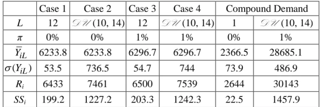
Table 1 numerically illustrates the four base cases and the case of compound demand, using data from the automotive industry. Here, n = 962, pi = 54%, L is fixed to 12 or 1 or is left random (discrete

uniform DU [10, 14]), and α = 0.01%; for compound demand, X = ⋅ + ⋅4 V₁ 6V₂, where V1 ~B (962L,

0.54) and V2 ~ B (962.L, 0.05), L = 1 or L ~ DU (10, 14), and π = 0% or 1% (in which case, Y

replaces X). Thus, we can obtain the order-up-to level Ri and safety stock SSi using the Monte Carlo

method, which is the only way to obtain a solution, except for case 1. These results, which we use hereinafter, show the impact of the increase of randomness due to the adjunction of random factors on the required safety stock.

Table 1. Numerical determinations of Ri and SSi., with α = 0.01%

Case 1 Case 2 Case 3 Case 4 Compound Demand

L 12 DU (10, 14) 12 DU (10, 14) 1 DU (10, 14) π 0% 0% 1% 1% 0% 1% iL Y 6233.8 6233.8 6296.7 6296.7 2366.5 28685.1 (Y_iL) σ 53.5 736.5 54.7 744 73.9 486.9 Ri 6433 7461 6500 7539 2644 30143 SSi 199.2 1227.2 203.3 1242.3 22.5 1457.9

In general, safety stock varies in the same direction as the coefficient of variation (ratio of the standard deviation of the demand distribution to its average) but opposite to the direction of accepted risk. Safety stock relations can be established when the order-up-to level is defined to meet the needs of an alternative or optional component in a BTS-SC in the steady state. We consider case 1 in which demand follows a binomial distribution B (nL, pi). In some conditions, especially when nLpi has a

sufficiently high value, an approximation of this distribution can be given by the normal distribution N (nLpi, pi(1−pi)nL). The definition of the standard normal variable tα is associated with a stockout

probability α, so the percentile R_iLα relates to tα according to the expected value of the demand

distribution, and its standard deviation is R_iLα =nLp_i+t_α nLp_i(1−p_i). The safety stock,

i iL

iL R nLp

SS α = α − , is then defined by SSiLα =tα nLpi(1−pi). Many industrial companies use the

concept of a safety coefficient to calculate safety stock. This safety coefficient refers to a constant to multiply with the demand average to calculate safety stock. We can express it as a function of the coefficient of variation, or p_i(1−p_i)nL/nLp_i= (1−p_i)/(nLp_i). The value of this safety coefficient is t_α (1−p_i)/(nLp_i), which leads to Equation 1

) 1 1 ( ) 1 ( i i i i i i iL nLp p t nLp p nLp t nLp R = + α − = + α − ; SSiLα =tα nLpi(1−pi)_. [1]

However, many companies cannot use the safety coefficient of an alternative component as a constant. That is, its use depends on the required risk protection, the size of the set affected by risk, and the probability of use of the considered alternative component.

If the probability of stockout before delivery is low, the expected value of the component shortage Is(RiLα) also is low. Therefore, the safety stock approaches the expected value of residual stock

before delivery. In general, the expectation Ir(RiLα) of residual stock at the end of a period with

demand XiL is given by Equation 2: ) ( I ) ( E ) ( Ir RiLα =RiLα − XiL + s RiLα . [2]

The order-up-to level RiLα must meet demand XiL, and Equation 2 is valid, regardless of the

probability distribution of XL. When the stockout probability is negligible, Is(RiLα) is close to 0,

which can be proved easily when an analytical relation of the expected value of the component shortage exists (e.g., normal or Poisson distribution). The average residual stock before delivery Ir(RiLα) is close to the safety stock RiLα−E(XL). The average residual stock and average stockout

vary in opposite directions and generate, respectively, carrying costs and stockout costs for the company. For example, with the data from case 1, when α = 0.01%, R1Lα = 6433, Is(R1Lα) = 0.001, and

Ir(R1Lα) = 199.24.

2.2. Safety stock of supplied components

Determination of the safety stocks of supplied components may depend on logistic constraints (e.g., batch size, limited transport capacity), which makes the definition of the rules of periodic replenishment policies more complicated. Before analyzing those cases, we examine the rules to use in a simple case in which the supply covers, without logistic constraint, a stochastic demand or a mix of stochastic and deterministic demand.

The order qjt for component j sent by B to A at the beginning of day t gets delivered at the

beginning of day t+Dj, where the due date is Dj and the lead time is λj (λj≤Dj). The inventory

position IPjt at the beginning of day t is the sum of the on-hand inventory observed Sjt, the kj expected

deliveries, and backorders. If the stockout probability is low, we can ignore the impact of unsatisfied demand (backorders or lost sales). No expected delivery exists (k_j =0) if the periodic replenishment review period is longer than the due date time (

j

j D

θ > ); otherwise, this number is positive and can

be noted as k_j =argmax(KK≤D_j/θ_j). The inventory position when ordering is

∑

₌ − + = kj h j t h j j S q

negotiated with supplier A (Pj ≤Dj), the order is based on statistical knowledge of anticipated

demand. Customer B has no interest in negotiating a due date superior to the lead time, because doing so, with the same stockout risk, increases safety stock. When Pj>Dj, if θj>Pj−Dj, the sent order

can be based partially on known demand. If θj≤Pj−Dj, the order is determined by known

requirements, and no safety stock is needed.

If no batch constraint needs to be taken into account when determining the order to send, supply is unit based. Batch-based supply is more complicated to define. In both cases, transport capacity limitations should be taken into account. In all cases, we assume that the accepted stockout risk α is predetermined and very low.

2.2.1. Unit-based supplies: Stochastic demand

The probability distribution is defined for demand j over the period (θ_j+λ_j), so it follows the law B

(

n(θ_j+λ_j),p_j

)

. If the normal approximation is possible, we use the distribution N

(

n(θ_j+λ_j)p_j, n(θ_j+λ_j)p_j(1−p_j)

)

. In this context, we can adapt Equation 1 to define the order-up-to level and safety stock:

, _{j j}, ( ) ( ) (1 ) j j j j j j j j R _{θ λ α+} =nθ +λ p +t_α nθ +λ p −p ; _{, ,} ( ) (1 ) j j j j j j j SS _{θ λ α+} =t_α nθ +λ p −p . [3]

If the lead time is random or quality is not guaranteed, we need a distribution generated by the Monte Carlo method to determine the order-up-to level associated with risk α. For example, assume that

θ = 2, λ ∼ DU (8, 12)→ θ λ+ ∼ DU (10, 14), n = 962, pi = 54%, and π = 1%; then, for α = 0.01%, Ri

= 7539 (see Table 1).

From a supply chain control perspective, two important observations emerge.

• If all alternative components assembled on the same workstation of end customer C are supplied by B, the total daily demand of alternative components is constant (n) because of its multinomial distribution. Therefore, the quantities ordered periodically equal θn. Plant B may need alternative

components j for its production, but if the components are all provided by the same supplier, the property of the constant total requirement remains valid. A supply of alternative components shared across several suppliers instead induces a periodic random total demand for each. This periodic load fluctuation may make the capacity commitment difficult for the supplier and induce additional costs.

• Supplier B might supply C with only a subset of what it needs, which creates a random amount of parts ordered from that supplier. In the same way, B can supply other clients with the same parts, which increases the variability of the demand to be satisfied by B. We cannot determine the demand distribution of component j used by different customers of B analytically, but we can

solve it using Monte Carlo methods. Simulation is essential for cases 2, 3, and 4 and for the case of compound demand. Moreover, with a quality problem, the generation of the random variable Z must be based on the sum of the demands generated for these customers.

2.2.2. Unit-based supplies: Stochastic and deterministic demands

We now consider the situation defined by a planning horizon P for customer B, which exceeds _j

the due date time D negotiated with supplier A of less than _j θ_j days (θ_j >P_j −D_j > ). The due 0 date time D is constant and can be equal to lead time _j λ_j. We assume that there is no quality problem. When an order is placed at the beginning of day t, to be delivered at the beginning of day

j

t+D to fill the needs of days t+D_j to t+D_j+

θ

_j −1, B knows with certainty its requirements for periods t+D_j to t+P_j −1, which are the needs of P_j−D_j days. The order sent on day t is the sum

of (1) a known quantity j 1 j h t P jh h t D x = + − = +

∑

, equal to the demand of P_j−D_j days, after delivery at the end of day t+D_j, and (2) a quantity q′ equal to the difference between an order-up-to level _jt

determined to meet a random demand with risk α and the inventory position. This demand is defined for a period of h days whose demands are unknown. Let K₁=arg max(K K≤(D_j+θ_j) /θ_j)be the number of replenishment cycles included in the decision horizon D_j+θ_j. Then, h cannot exceed

1

(D_j+θ_j−K P( _j −D_j))and does not obtain this value if the requirement for day t was known when the order was sent to cover that demand as the requirement of the previous day; rather, it obtains this value if

3 2

K >K , with K₂=arg min(K K≥(D_j+1) /θ_j) and K₃=arg min(K K≥P_j /θ_j). Then,

2

(P_j−K ⋅θ_j)is subtracted from (D_j+θ_j−K P₁( _j−D_j)). The order to send at the beginning of day t is the sum of the following:

• j 1 j h t P jh h t D x = + − = +

∑ , which corresponds to the demands of the (P_j−D_j)days following the delivery; • q′ , or the difference between the order-up-to level _jt R_jhα and the inventory position IP′ at the _t

beginning of day t; R_jhα, or the percentile defined for risk α of the random variable X_j  B

(nh p, _j), with h=_D_j +θ_j −K P₁( _j −D_j)_{ } − (K₃−K₂)(P_j −K₂⋅θ_j)_{ ; and} IP′ , which is an _t

inventory position that does not take into account all the firm orders known when ordering.

j

X  B ( , )nh p_j with h=_D_j +θ_j−K P₁( _j −D_j)_{ } − (K₃−K₂)(P_j −K₂⋅θ_j)_{ , where}

1 arg max( ( j j) / j)

K = K K≤ D +θ θ ,K₂=arg min(K K≥(D_j+1) /θ_j),

For example, for component j= , with 1 θ₁= , 6 D₁= , and 11 P₁= , we obtain 13 K₁= , 2 K₂= , 2

3 3

K = , and h=

[

11 6+ −2(13 11)−

] [

− (3−2)(13− ⋅2 6)

]

=12. With X₁ B (12 962,0.54)⋅ , we obtain

1,12,0.01% 6433

R = (see Table 1). For example, an order placed at the beginning of day t=51 will be delivered at the beginning of day t=51 11 62+ = and must fill the needs of 6 days (days 62 to 51 11 6 1 67+ + − = ). At the beginning of day t=51, the demands of days 51 to 63 ( 51 13 1)= + − are known; however, although the needs of days 62 and 63 are also known exactly, the needs of days 64 to 67 are only known in probability. The expected delivery at the beginning of day 56, triggered by the order sent at the beginning of day 45, involves the knowledge of demand of days 56 to 57; the past delivery sent at the beginning of day 50 involves the knowledge of demand of days 50 to 51. Thus, the demand of 11 6 17+ = days (from days 51 to 67) is covered with deliveries made at the beginning of days 50, 56, and 62 and is triggered by orders made at the beginning of days 39, 45, and 51 that applied the exact knowledge of the demand of 5 days (51, 56, 57, 62, and 63). The stochastic demand to consider now is the 17 5 12− = days’ demand. We assume that when the order is defined at the beginning of day 51, the following information is known: (1) the inventory position is 3,555 units; (2) the order delivered on the previous day included the knowledge of the demand of day 50 (487); (3) the delivery of 3,109 units, expected at the beginning of day 56, includes the known demands of days 56 and 57 (492 and 540 units); and (4) the known demands of days 62 and 63 are 506 and 515 units. Then, the order is (506+515)+(6433−

{

2593 3109+ −487−492 540 )−

}

=3271units.

If we exclude the possibility of lost sales, q′ equals the sum of observed demand on the last _jt

(

θ_j −(P_j−D_j)

)

days before day t, 1

j j j h t jh h t θ P D x = − = − + −

∑ . In Equation 5, we summarize the determination of the order to send in the steady state, with a mix of stochastic and deterministic demand: 1 ₁ j j j j j h t P _{h t} jt _{h t D} jh _{h t P D} jh q =

∑

= + −_{= +} x +

∑

_{= − + −}= −_θ x with

θ

_j>P_j−D_j >0 . [5]

To take quality into account (case 3), we must use the simulation to obtain the probability distribution and thereby determine the percentile. To define variable Z , we assume that the quality _j

problem exists for all orders and sum random demand together with firm orders. By doing that, the distribution to use changes at every decision. A less efficient but good solution can be used instead: in a steady state, these firm orders are random variables that follow a binomial law with the same probability used to address the random needs accounted for in the order. In the Monte Caro simulation, Z_j uses outcomes from the distribution B

(

n D( _j+θ_j),p_j

)

, and Equation6 becomes the following:

j j j

Y =X +Z , where X given by [4], _j Z_j  BN (U_j,π_j) and U_j  B

(

n D( _j+θ_j),p_j

)

In the previous example, if π₁=1% instead of 0%, the order-up-to level become 6603.

Next, we assume that the lead time λ_j is random and that the quality of the delivered items is guaranteed (case 2). If the maximum value of λ_jdoes not exceedD , considering the randomness of _j

j

λ is useless. Otherwise, it is preferable to discard the due date and replace D_j with λ_j. However,

the randomness of λ_j involves the randomness of _K P₁( _j−D_j)+(K₃−K₂)(P_j −K₂⋅θ_j)_{ , which is} the number of firm orders known when ordering. This prevents any analytical solution from defining the order as the sum of q′_jt and firm orders beyond λ_j, whose number is random. An operational solution is to ignore the information given by the firm orders and use the solution previously discussed in Section 2.2.1.

2.2.3. Batch-based supplies

External supply often depends on batch constraints. Each order sent may be a multiple of the number κ of units used in transport, as models of stock determination note. In stochastic inventory models, the analytic solution is characterized by a double inequality for the cumulative probability of two successive discrete values, multiples of κ. They enclose an optimal target probability, depending on the structure of the costs used in the objective function of the model. Because inventory models are too simplistic to cope with the encountered complexity in an USC, it is preferable to use provisioning rules that guarantee a low stockout probability α. If the order sent corresponds to the greatest multiple of κ, respecting the condition of a stockout probability inferior to α (i.e.,

.arg min(K K (R_j PS_j) / )

κ ≥ − κ ), the protection against stockout risk is excessive. If the order sent corresponds to the smallest multiple κ, leading to a stockout probability superior to α (i.e.,

.arg max(K K (R_j PS_j) / )

κ ≤ − κ ), the protection against stockout risk is insufficient. The multiple to choose depends on an accepted reasonable risk β, greater than α and sometimes incurred because of batch limitations. From case 1, we assume that the transport container contains κ = 18 units. With α = 0.01%, we find R_j= 6433. If we accept risk β = 0.015%, then P(Xi > R_jβ) ≤ 0.015% gives R_jβ

= 6427. For example, with PSj = 6242, the quantity to order without batch constraint is

6433 6242 191

q′= − = ; the batch constraint leads us to order either 180 or 198 units. In the first case, the implicit order-up-to level is decreased by 191 180− =11, which yields a stockout risk higher than β (0.021%), and thus 198 units are to be ordered. If (R_j −PS_j)−κ.arg max(K K≤(R_j−PS_j) / )κ is

less than R_j−R_jβ (e.g., 6), the choice of .arg max(κ K K≤(R_j −PS_j) / )κ leads to a risk that is not greater than β. That is,

.arg max( ( ) / ), ( ) .arg max( ( ) / )

j j j j j

q =κ K K≤ R_j−PS_j κ if R −PS −κ K K≤ R_j−PS_j κ ≤R −R _β

else q_j =κ.arg min(K K≥(R_j−PS_j) / )κ [7]

2.2.4. Incurred risk and transport capacity limitations

The means of transport usually have limited capacity, G. The ordered quantity cannot exceed this limit (→Max R( _j−PS G_j, ) without batch constraints). Therefore, the incurred stockout risk is higher than desired, unless there is virtually no chance that demand exceeds this capacity. In this case, transport may be less efficient. To preserve the target risk level α, it is necessary to increase the order-up-to level, which we can do easily with a dichotomous method. If n = 962, p_j = 54%, θ = 2, λ = 10,

and α = 0.01%, we find R = 6433 (see Table 1). If G = 1045, a simulation of this periodic _j

replenishment policy (with backorders) for 50 million iterations leads to a risk of 0.576% and a stockout average of 0.228. To keep α = 0.01%, it is necessary to fix R to 6598. The safety stock _j

then increases from 199.2 to 364.2. This simulation widens the scope of the analysis from a local optimization to a more global one that includes transport, carrying, set-up, and stockout costs. A batch limitation is more complicated to take into account but very tractable. The transport capacity limitation is necessarily a multiple of packaging size, especially in the case of homogeneous products.

2.3. Safety stock of produced components

We next focus on the production of a product i by unit B, in response to demand from customer C. In this context, we assume that the lead time λ_i between the start of production and the component’s appearance in stock of plant B is constant. The lead time corresponds either to cycle time, if a set of different components is launched in production, or to production time, if only one component is launched. Customer C sends B its orders for i at the beginning of the day, every

θ

_i days. The order received at the beginning of day t must be sent at the end of day t+D_i. With a lead time

λ

_i, B has

i i

D −

λ

days to produce and send the order (D_i ≥

λ

_i). Component i gets integrated into the production cycle of H days. The production of component i finishes F_i days after the beginning of the cycle. If this cycle includes only component i, it is obvious that H =F_i, and there is no reason to synchronize deliveries (all

θ

_i days) or launches in production (all H days). We first consider a build-to-stock production, then a build-to-order production, and finally a combined production process.

2.3.1. Build-to-stock production

The rules used for build-to-stock production depend on the values taken by the production cycle and the replenishment cycle, as well as the idea that the production decision depends on one or several

components. First, we assume either that the production cycle H is shorter than the replenishment cycle

θ

_i (→H≤

θ

_i) and that the order from customer C is immediately executable (Di−λi= 0) or

that the time remaining before delivery is less than the replenishment cycle

θ

_i (→D_i− ≤

λ θ

_{i i}). The distribution to determine the order-up-to level is the binomial distribution B (n

θ

_i,p_i). In a steady state, the quantity that B launches into production is equal to the last quantity sent to C; it is a random variable. However, if the supplier produces all alternative references assembled on the workstation of the customer assembly line, ordered at the same time (→ = ∀

θ θ

_i , i), the sum of ordered quantities is constant (nθ ) because demand for alternative components follows a multinomial distribution.

Second, if H > and the time remaining before delivery is less than the production cycle θ_i

(D_i− <λ_i H), we can distinguish two cases depending on the number of products manufactured in the production cycle. If product i is the only one to be manufactured in this production cycle, H = . F_i

When the order is sent at the beginning of day t to be delivered on day t+H− , the inventory 1 position IP of component i, increased by the quantity launched _it q_it =R_it−IP_it, should meet demand until the end of the next production cycle, on day t+2H. The number of deliveries during a period of 2H days must be between η_1i =argmax(K K<2H/θ_i) and η_2i=argmin(K K>2H /θ_i). For example, with H = 5 and

θ

_i= 4, the number of deliveries is either 2 or 3. If 2H is a multiple of

θ

_i, the number of deliveries during a 2H-days period is constant. The distribution to determine the order-up-to level is binomial B(nηθi, pi), with η η= or ₁ η η= ₂. It can often be approximated by

N(n

ηθ

, 2n

ηθ

_{i i}p (1−p_i)). For example, if B receives orders every four days from C (θ_i =4)and Fi

= five days, the distributions are B( 962 2 4, 0.54⋅ ⋅ ) and B( 962 3 4, 0.54⋅ ⋅ ). When α = 0.01%, the order-up-to level is 4,318 (two deliveries) or 6,433 (three deliveries). A lack of synchronization between cycles H and θ leads to periodic variation in the production. The quantity to be launched in production by B equals the sum of quantities previously shipped to C only if the order-up-to level used for the production launch is the same as that used previously. The sum of the quantities launched varies strongly when the number of deliveries since the previous launch changes (as a result of change in η). This sum equals n⋅ ⋅ only if the order-up-to levels have not changed since the previous η θ launch and B produces all alternative components.

If several components are launched and are to be produced successively during the same production cycle (→ = ∀

θ θ

_i , i), an order sent at the beginning of day t increases the inventory position IPit of component i by the quantity launched in production q_it=R_it−IP_it, to be delivered at

the beginning of day t+ . It should meet demand until the next delivery, at the beginning of day H

i

1i arg max(K K (H Fi) / )

ν = < + θ and ν_2i=arg min(K K>(H+F_i) / )θ . If θ= , 4 F_i= , and 2 5

H = , the number of deliveries is either one or two. If (H+F_i) is a multiple of θ, the number of deliveries over H + days is constant. The distribution for determining the order-up-to level is F_i

binomial, B(n

νθ

,p_i), with

ν ν

= ₁ or

ν ν

= ₂. The distribution can be approximated by N

(

nνθ, 2nνθp_i(1−p_i)

)

in many cases. Our previous remarks about the variability of production remain valid. In our example, the distributions are laws, B( 962 2 4, 0.54⋅ ⋅ ) and B( 962 1 4, 0.54⋅ ⋅ ), which lead to order-up-to levels for α = 0.01% of 4,318 (two deliveries) or 2,193 (one delivery), causing oscillations in the USC.

2.3.2. Build-to-order production

Now assume that the replenishment cycle θ_iis not lower than the production cycle (→H ≤θ_i) and is greater than the supplier anticipation (→D_i−λ θ_i> _i). Production can be made to order, and a production launch involves no more than one delivery. The maximum number of canceled consecutive launches is arg min(K K>(D_i−λ_i) /H). For example, if H = 5,

θ

_i =12, and

(D_i−

λ

_i) 14= , the maximum number of null consecutive launches is 2. If H >

θ

_i and if supplier anticipation is at least twice the production cycle (→(D_i−

λ

_i)≥2H), production also can be made to order. In this context, it is possible to launch a production quantity that can be delivered during the following production cycle, as well as one or more subsequent deliveries if anticipation is sufficient. However, it is preferable to smooth the load and launch only deliveries for the following production cycle. Again, the number of deliveries to consider can vary between two production cycles: at least 1 and no more than arg min(K K≥(D_i− −λ_i H) /θ_i). If H = 5,

θ

_i =3, and D_i− =

λ

_i 11, no more than the quantity of two successive deliveries should be launched.

The irregularity of the number of launches and the quantities launched leads to disorganization. However, this can be eliminated if the production cycle equals the periodic replenishment review period but remains less than supplier anticipation (→(D_i−

λ

_i)>

θ

_i). Quantities vary from order to order because they correspond to quantities consumed, whose distribution is binomial. However, if the supplier produces all alternative components for the customer’s assembly line, the sum of ordered quantities is constant (nθ). If this supplier has multiple customers for all or some produced components, the condition extends to each customer.

2.3.3. Mixed production

Previously, we showed that (1) if (H≤ ), production must be built to stock if (θ_i D_i−λ_i)≤ and θ_i made to order otherwise (D_i−λ θ_i > _i), and (2) if H > , production can be built to order if θ_i

(D_i−λ_i)≥2H. If H> and θ_i H<(D_i−λ_i)<2H, production may be a combination of built to order and built to stock. The analysis of these possible configurations is similar to that for build-to-stock production, except that only µ deliveries to the customer on (D_i−λ_i) days after the production launch of component i on day t are known. They can be covered by a build-to-order production. The number µ is either

µ

₁=arg max(K K<(D_i−

λ θ

_i) / _i) or

µ

₂=arg min(K K>(D_i−

λ θ

_i) / _i). Therefore, the difference, which could be null, between η and µ corresponds to deliveries that can be covered by a build-to-stock production. We assume that (D_i−λ_i)= , 7 θ_i= , and 4

5

H = (→µ₁=1,µ₂= . The inventory position updates with a decision to integrate known firm 2) orders from the customer and deliveries for later orders. In this example, if both a production cycle and a replenishment cycle start at the beginning of day 1 and if a production order is delivered on day 1, quantities launched in production at the beginning of day 1 must cover an unknown order (day 8 → build-to-stock); quantities launched in production cycle 2 (day 6) must cover an unknown order (day 12 → build-to-order); and quantities launched in production cycle 3 (day 11) are partly made-to-order (firm order of day 16) and partly made-to-stock (unknown order of day 20).

3. Restoring steady-state performance in a changing environment

If managers of upstream USC links can adapt their decision rules quickly using appropriate information transmitted from the final assembly line, steady-state performance, in terms of efficiency and effectiveness in a decentralized management of USC plants, can be maintained even if the environment changes. We explain why this information is the result of a double transformation that relies on mechanisms associated with the BOM explosion and time lags. The latter pertains to the growing delay of moving upstream in the supply chain, that is, between the date of production of a component by one link and its integration into the end product in the final assembly line. Without this double transformation, the information transmitted is meaningless. In the steady state, the time lag mechanism (which we describe subsequently) does not play an important role, because when the decision rules have been defined using appropriate information, there is no reason to change them. If every link receives appropriate information and uses it to control stockouts, disturbances in the supply chain should be rare, and the managerial independence of each link of the USC can be guaranteed. Therefore, we move on to check various implementation problems.

3.1. Double transformation of information

We begin by determining the information required by each link of the USC, according to the steady-state assumption, to establish production and replenishment rules that will allow for both management independence and smooth USC functioning. Such rules also indicate the initial calibration of the steady state of the USC. We then show that knowledge of current or previous

changes enables the adaptation of monitoring rules to maintain steady-state performance. This point leads to a conceptualization of an extended OPP that completes the OPP.

3.1.1. Mandatory use of planning BOM to define information to send upstream

Different forms of information sharing are useful for decreasing costs and risks in short-term decision making (Chandra et al., 2007). Firms can share raw information, such as sales histories, orders, inventory positions, and deliveries, or they can share processed information related to planned or forecast demand (Ryu et al., 2009). The latter might be the output of a collaborative process that represents a first step toward the centralized management of the supply chain.

The value of shared information depends on not only its possible but also its effective uses, which aim to share cost savings across the supply chain. Even in the steady state, transmitting detailed information about daily production or end-user demand to upstream echelons is useless: Products exchanged between links in the USC are not the same, unlike in downstream echelons, because of the classic mechanism of BOM explosion.

Consider the mechanism of requirement along the USC. We assume, in a first stage, that all the components are produced to stock and the steady-state assumption holds (we remove these restrictions later). Demand for a component is pulled by one of the alternative parts mounted in a workstation used in the final assembly line; for example, the same piston might be found in various motors on the car assembly line.

The planning BOM describes related options or modules that constitute an average end item. Applied to a set of R alternative components r that might be mounted in a given station of the assembly line (e.g., motors), the planning BOM coefficients pr ( 0< p_r <1,

∑

_rp_r =1) represent the

steady-state probabilities of a multinomial distribution, in which the number of trials n equals the daily production of cars. These alternative components belong to the first level of the BOM. The daily demand X_1r of the alternative component r follows the binomial distribution B(n p, _r), because in n trials, the event “alternative component r is mounted” gets tested against the event “component r is not mounted.” Component r may include a_rs >0 units of component s (e.g., piston set) in the second level. The daily demand X_2rs of component s, as induced by the daily requirement X_1r, is a_rs⋅X_1r. If component s is used by several alternative components r′∈Rs, the total demand X2s is as follows:

2s r R_s 2r s r R_s r s 1r

X =

∑

_′∈ X _′ =

∑

_′∈ a _′ ⋅X _′

. [8]

Knowledge of the distribution of X_2s is necessary to define the appropriate order-up-to level of component s based on the required stockout risk and its safety stock. The distribution of the sum of weighted binomial variables can be defined easily using a Monte Carlo simulation. Gross requirements are random variables, not fixed values, as in the MRP computation of planned orders.

In turn, the component s of the second level (e.g., a given piston set) uses b_su( 0)> components u from the third level, though it may not be the only one

(

→s′∈S_u

)

. The previous reasoning applies again, after we link component u to component r: Demand X_3u is a weighted sum of the subset of demands of components from the first level:

3u s S_u 3s u s S_u s u 2s s S_u s u r R_s r s 1r

X =

∑

′∈ X ′ =

∑

′∈ b′ ⋅X ′ =

∑

′∈ b′

∑

′∈ _′a ′ ′⋅X ′_. [9]

Again, its distribution can be defined only with a Monte Carlo simulation.

To illustrate, we consider the following example: For a given set of six alternative motors (r = 1, …, 6) that can be mounted in a workstation of a car assembly line, the motors’ planning BOM is {M1

54%; M2 13%; M3 4%; M4 22%; M5 5%; M6 2%}. The line production is 962 cars per day

(→ n=962). The daily requirement X1r of the alternative component r follows the binomial

distribution B(962; pr), such that X1,1 ∼ B (962; 54%) for motor 1 and X1,5 ∼ B (962; 5%) for motor

5. In the steady state, with a risk of 0.01%, the safety stocks of motors 1 and 5 are 57.5 and 26.9, respectively. If, according to the BOM, only motors M1 and M5 include the piston set P1 (s = 1) and

M1 needs 4 piston sets while M5 needs 6 piston sets (a1,1 = 4; a1,5 = 6), the daily requirement for piston

set P1 is

X

2,1

=

4

X

1,1

+

6

X

1,5, which is an even discrete variable that starts from 4 for positive values

2,1

( X = 0, 4, 6, 8, …, because X1,1 and X1,1 are discrete nonnegative values). Using the Monte Carlo

simulation, we find a reorder point of 2,644 (risk = 0.01%) and a demand average of 2,366.5; the safety stock of piston sets is 277.5. If only piston sets P1 and P3 include the piston head H1, which is

component (u = 1) of the third level, and P3 is mounted only in motors M2 and M6, the daily

requirement of piston set P3 is X2,3=4X1,2+4X1,6. With b1,1 = b1,3 = 1, the daily requirement of H1 is

a sum of four weighted binomial variables

3,1 1 (4 1,1 6 1,5) 1 (4 1,2 4 1,6) 4 1,1 6 1,5 4 1,2 4 1,6

X = ⋅ X + X + ⋅ X + X = X + X + X + X , where X1,1 ∼ B (962; 54%), X1,5 ∼ B (962; 5%), X1,2 ∼B (962; 13%), and X1,6 ∼ B (962; 2%). Again using Monte Carlo

simulation, we can show that in the steady state, the average demand for piston heads H1 is 2,944 and

the safety stock is 326.

3.1.2. Mandatory use of time-lag mechanisms for a nonpersistent steady state

The steady state never lasts more than a few weeks, but environmental changes are often slow enough to suggest that a real-world scenario will be defined by a succession of slightly different steady states. From one state to the next, changes pertain to the level of production and the structure of demand for each set of alternative components. Consider a component launched in production at time t in a USC echelon and integrated in a vehicle at time t + δ.

To make effective decisions at time t, the echelon needs appropriate information for time t + δ, such that δ represents the information lag. This lag plays a similar role to the lead time lag in the MRP

but spans across the wider perimeter of the USC. In addition, in contrast with the MRP system, we assume we are beyond the OPP (δ > OPP) and, thus, beyond the MRP frozen horizon. Therefore, the mechanism we described in the previous section must be adapted. To simplify the mechanism description, we assume that component productions are launched every day for all components produced in the USC; the replacement of that assumption is easy but yields a more complex formulation. The demand X_1rt of the alternative component r of the first level in day t, to launch in production that day, follows the binomial distribution B ( _{1 ,} ; _{1 ,}

r r

r t r t

n _+δ p _+δ ), because those components will be integrated into a vehicle at time t + δr. Demand X_2st of the alternative

component s of the second level for day t, as used by several alternative components r′∈R_s, is a weighted sum of a subset of the daily production of components in the first level, using the information lags

δ

_{r s′} , which may differ. Then, Equation 10 replaces Equation 8:

2st r R_s 2r st r R_s r s 1 ,r t _{r s}

X =

∑

_′∈ X _′ =

∑

_′∈ a _′ ⋅X _{′ +δ′}

. [10]

Component s of the second level uses component u of the third level

(

→s′∈S_u

)

. After linking component u to component r, demandX_3ut is again a weighted sum of a subset of daily production of components in the first level, with information lags

δ

_{r u′} that may differ. Then, Equation 11 replaces Equation 9:

3ut s S_u 3s ut s S_u s u 2 ,s t _{r u r s} s S_u s u r R_s r s 1 ,r t _{r u}

X =

∑

′∈ X ′ =

∑

′∈ b′ ⋅X ′ +_δ′ −_{δ′ ′} =

∑

′∈ b′

∑

′∈ _′a ′ ′⋅X ′ +_{δ′ .} [11] Again, the distributions can be defined easily using a Monte Carlo simulation.

We adapt our previous example to introduce the current day t. Motors 1 and 5 are characterized by information lags of 2 and 3 days, respectively (→ motors 1 and 5 produced on day t are mounted in the assembly line on days t+ and 2 t+ , respectively). We assume that the multinomial distribution 3 and production level do not change during the first two days and that, thereafter, daily production decreases from 962 to 605, and the motors’ planning BOM become {M1 49%; M2 10%; M3 3%; M4

25%; M5 11%; M6 2%}. With this information, we can determine that the production of M1 and M5 on

day t reflects the requirement of the assembly line for days t+ and 2 t+ : 3 X1,1,t+2 ∼ B (962; 54%)

and X_1,5,t+3∼ B (605; 11%). With a risk of 0.1%, the safety stock is still 47 for M1 and 34.5 for M5.

If, for the production of piston sets H1, the delay between the planned order and delivery is two days,

the part of the production of day t sent to produce M1 will be set by a car using M1 four days later

(information lag); the other part is sent to produce M5 five days later. Demand for piston set P1 on day t is X_2,1,t =4X_1,1,t+4+6X_1,5,t+5, where X_1,1,t+4 ∼ B (605; 49%) and X_1,5,t+5∼ B (605; 11%). Using

the Monte Carlo simulation, we calculate that the safety stock of piston sets is 190.8 for that production day (average demand of 2477.2).