ÉCOLE DE TECHNOLOGIE SUPÉRIEURE UNIVERSITÉ DU QUÉBEC
THESIS PRESENTED TO
ÉCOLE DE TECHNOLOGIE SUPÉRIEURE
IN PARTIAL FULFILLMENT OF THE REQUIREMENTS FOR A MASTER’S DEGREE IN MECHANICAL ENGINEERING
M. Eng.
BY Joël BÉDARD
IMPROVEMENT OF SHORT-TERM NUMERICAL WIND PREDICTIONS
MONTRÉAL, SEPTEMBER 16 2010 © Copyright 2010 reserved by Joël Bédard, 2010
BOARD OF EXAMINERS
THIS THESIS HAS BEEN EVALUATED BY THE FOLLOWING BOARD OF EXAMINERS
Dr. Christian Masson, Thesis Supervisor
Département de génie mécanique à l’École de Technologie Supérieure
Dr. Yves Gagnon, Thesis Co-supervisor
Faculté des études supérieures et de la recherche à l’Université de Moncton
Dr. Wei Yu, Thesis Co-supervisor
Meteorological Research Division at Environment Canada
Dr. Robert Benoit, President of the Board of Examiners
Département de génie mécanique à l’École de Technologie Supérieure
Dr. Stéphane Bélair, External Examiner
Meteorological Research Division at Environment Canada
THIS THESIS HAS BEEN PRESENTED AND DEFENDED BEFORE A BOARD OF EXAMINERS AND PUBLIC
SEPTEMBER 2ND 2010
ACKNOWLEDGEMENTS
This project, part of the Wind Energy Strategic Network (WESNet), is funded by the Natural Sciences and Engineering Research Council (NSERC) of Canada, and by the Canada Research Chair in the Aerodynamics of Wind Turbines in Nordic Environment (École de Technologie Supérieure), the K.-C.-Irving Chair in Sustainable Development (Université de Moncton) and the Environmental Numerical Prediction Research Section of the Meteorological Research Division (Environment Canada). The author also acknowledges the contributions of the Wind Energy Institute of Canada (WEICan) in this research program.
On a personal note, I wish to thank my directors Christian Masson, Yves Gagnon and Wei Yu for their advices and support in carrying out this work. More specifically, I am grateful to have had Christian Masson give me the opportunity to work in his lab and to Yves Gagnon for introducing me to different parties involved in the wind energy sector. Also, a very special thanks to Wei Yu for his scientific supervision and his devotion to the project: he integrated me into the Meteorological Research Division team at Environment Canada. Thanks to André Plante, Laurent Chardon, Djamel Bouhemhem and others colleagues from the Meteorological Research Division team for their technical support and advices. Also, thanks to Nicolas Gasset and Robert Benoit from the Canada Research Chair in the Aerodynamics of Wind Turbines in Nordic Environment (École de Technologie Supérieure) for many fruitful discussions.
Moreover, I wish to thank the WEICan staff and Mathieu Landry from the K.-C.-Irving Chair in Sustainable Development (Université de Moncton) for their technical support with atmospheric measurements and their warm welcoming during my stay in the Maritimes. I am also grateful to Linda Mallette (École de Technologie Supérieure) for her precious help with the official recognition of the competencies acquired at Université de Moncton. Also, thanks to the members of the present jury for their precious comments and their judicious evaluation. On a final note, very special thanks are reserved to my family and my friends for being with me, for your constant support and your infinite patience. Thank you very much!
IMPROVEMENT OF SHORT-TERM NUMERICAL WIND PREDICTIONS Joël BÉDARD
RÉSUMÉ
Avec la croissance soutenue de l’énergie éolienne sur les marchés énergétiques, les opérateurs des réseaux électriques ont de plus en plus de défis à relever en matière d’équilibrage de réseau, le tout afin de minimiser les coûts associés à la gestion des autres sources énergétiques. Le vent étant une source énergétique variable, la prévision de la puissance éolienne est donc l’une des solutions qui permettra à ce type d’énergie de devenir viable du point de vue économique, tant sur les marchés régulés que dans les marchés ouverts. Dorénavant, il semble qu’il y ait un besoin urgent pour des modèles permettant de prédire de manière fiable la puissance éolienne à court-terme (0 – 48 h); ceci, afin de maintenir l’intégration de l’énergie éolienne dans le portefeuille énergétique des différentes juridictions.
En fonction des besoins de l’industrie éolienne, « Environnement Canada » effectue, depuis trois ans, des prévisions météorologiques expérimentales dans l’est canadien à l’aide d’un modèle de prévisions numériques à aire limitée (GEM-LAM 2.5 km). La région couverte englobe la péninsule gaspésienne ainsi qu’une partie des provinces maritimes. Cette région couvre plusieurs sites éoliens tels que North Cape. Ce site est situé à l’Ile du Prince Édouard où le Wind Energy Institute of Canada opère un centre d’essais éolien. Une analyse préliminaire des prévisions et une inspection minutieuse de ce site ont permis de démontrer que, bien que la résolution du modèle soit déjà relativement haute, elle manque tout de même de raffinement afin de bien représenter les phénomènes météorologiques pour ce site côtier à topographie complexe. Pour cette raison, un module géophysique de traitement statistique des sorties (Geophysic Model Output Statistic (GMOS)) a été développé et appliqué afin de permettre une optimisation de l’utilisation du modèle de prévision météorologique à des fins de prévision de la puissance éolienne à court-terme. GMOS diffère des MOS couramment utilisés dans les centres météorologiques par les aspects suivants : 1) il prend en compte les paramètres géophysiques régionaux (hauteur topographique, rugosité de surface, etc.) ainsi
que la direction du vent; 2) il peut être directement appliqué pour corriger les sorties de différents modèles numériques sans entraînement, bien qu’un entraînement soit bénéfique.
Ce module statistique a été entrainé et testé pour le site de North Cape, où il a réduit l’erreur quadratique des prévisions de 25 à 30 %. Cette amélioration significative est observable pour tous les horizons temporels ainsi que pour la majorité des conditions météorologiques. De plus, la signature topographique de l’erreur de prévision a été éliminée suite à l’application du GMOS. D’ailleurs, le modèle de prévision numérique combiné au GMOS offre une prévision supérieure à celle de la persistance dès un horizon de 2 h. Ce gain n’était observable qu’à partir d’un horizon de 4 h sans l’utilisation du GMOS. Enfin, une validation effectuée pour un site établi à Bouctouche (Nouveau Brunswick), présentant des améliorations similaires des prévisions de vent de surface, a permis de démontrer l’applicabilité générale de la méthode.
Cette étude, présentant un module statistique permettant l’optimisation de l’utilisation des prévisions météorologiques à haute résolution, a aussi contribué au développement d’une méthodologie afin de mieux comprendre les erreurs de prévisions reliées aux différentes conditions météorologiques. Cet outil d’analyse a permis d’évaluer la contribution d’erreur de phase et d’amplitude pour des conditions atmosphériques normales ainsi que pour divers évènements météorologiques à caractère dynamique tels que les variations subites de vitesse du vent, le passage de dépressions etc. Une compréhension accrue des erreurs de prévisions ainsi que l’acquisition de prévisions éoliennes plus précises permettront d’augmenter la valeur économique de l’énergie éolienne sur le marché.
Mots- Clés : énergie éolienne, prévision de puissance, prévisions numériques, couche limite atmosphérique, vent de surface, sites complexes, statistiques de sortie, analyse d’erreur
IMPROVEMENT OF SHORT-TERM NUMERICAL WIND PREDICTIONS Joël BÉDARD
ABSTRACT
With the sustained growth of wind energy installed capacity for electricity generation, electricity system operators have increasing challenges balancing the electricity grid, notably in regards to minimizing the cost of other energy sources dispatch. Due to the variability of wind, wind power generation forecasting is an important issue for the economic viability of wind energy, whether in regulated or open markets. Therefore, there is a pressing need for robust short-term (up to 48 hours) surface wind forecast models, and eventually wind power forecast models, in order to sustain the integration of wind energy in electricity portfolios of jurisdictions.
Computed for the needs of the wind energy industry, three years of experimental meteorological forecasts in Eastern Canada are available from Environment Canada Numerical Weather Prediction (NWP) model configured on a limited-area (GEM-LAM 2.5 km) for wind power predictions. These data include forecasts for the region of North Cape (Prince Edward Island) where the Wind Energy Institute of Canada runs a test site for wind turbines. Although the model spatial resolution is already relatively high (2.5 km), preliminary statistical analysis and site inspection revealed that the model does not have sufficient grid spacing refinement to properly represent the meteorological phenomena on this complex coastal site. For this reason, a Geophysic Model Output Statistic (GMOS) module has been developed and applied to optimize the use of the short-term NWP. GMOS differs from other MOS that are widely used by meteorological centers in the following aspects: 1) it takes into accounts the surrounding geophysical parameters such as surface roughness, terrain height, etc. along with the wind direction; 2) GMOS can be directly applied for model output correction without any training although a training of the GMOS will further improve the results.
This statistical module was trained and tested over the North Cape site and it basically improves the predictions RMSE by 25 – 30 % for all time horizons and almost all meteorological conditions. Also, the topographic signature of the forecast error due to insufficient grid refinement is eliminated and the NWP combined with the GMOS now outperforms the persistence model after a 2 h horizon, instead of 4 h without the GMOS. Ultimately, in order to generalize the results, this methodology has been validated by an independent test case performed on a site located in Bouctouche (New Brunswick). Similar improvements on the GEM-LAM 2.5km forecasts were observed thus, showing the general applicability of the GMOS.
Although the current study presents an optimization of the use of short-term NWP for wind power forecasts using a statistical module, it also contributes to the development of a methodology and an analysis tool to assess and understand the NWP uncertainties on the amplitude and the phase of the surface wind forecast errors for different meteorological situations. A better knowledge of the wind speed and wind power forecast uncertainties, along with more accurate short-term wind forecast models, will increase the economic value of wind energy on the market.
Keywords: wind energy, wind power forecast, numerical weather prediction, atmospheric boundary layer, surface wind, complex sites, model output statistics, uncertainty analysis
TABLE OF CONTENT
Page
INTRODUCTION ...1
CHAPTER 1 LITERATURE REVIEW ...4
1.1 Numerical wind power prediction models ...4
1.2 Model output statistics ...5
1.3 Reference models ...5
1.4 Performance evaluation of models ...6
1.5 Benefit of ensemble forecasts ...8
1.6 Challenges to overcome ...9
CHAPTER 2 MEASUREMENT DATA ...11
2.1 Data quality analysis ...14
2.2 Anemometer selection ...25
2.3 Atmospheric measurement uncertainty ...28
2.4 Wind characteristics ...33
CHAPTER 3 VERTICAL INTERPOLATION OF THE FORECASTS ...39
3.1 Power Law profiles ...39
3.2 Linear profiles ...40
3.3 Logarithmic profiles...40
3.4 Comparison of the different vertical interpolations ...42
CHAPTER 4 NUMERICAL WEATHER PREDICTION MODEL ...50
4.1 Model outputs ...50
4.2 Stability parameter computation ...51
4.3 Preliminary analysis ...53
CHAPTER 5 GEOPHYSIC MODEL OUTPUT STATISTICS ...57
5.1 Reference interpolation method ...57
5.2 Geo-referenced weighting module ...59
5.3 Linear regressions ...64
5.4 Artificial Neural Networks ...67
5.5 Model verification ...70
5.6 Comparison of the different GMOS ...73
CHAPTER 6 STATISTICAL ANALYSIS AND NWP MODEL VALIDATION ...81
6.1 Assessment of the phase and amplitude error contributions ...81
6.2 Validation of the error assessment methodology ...83
6.3 Assessment of the forecast errors for complex sites (NWP with GMOS) ...87
ANNEX I DATA RECOVERY RATE AT THE BOUCTOUCHE SITE ...98
ANNEX II ANEMOMETER RELIABILITY AT THE BOUCTOUCHE SITE ...99
ANNEX III CHARACTERISTICS OF THE WIND AT THE BOUCTOUCHE SITE ....100
ANNEX IV VERTICAL INTERPOLATION AT THE BOUCTOUCHE SITE ...105
ANNEX V COMPARISON OF THE GMOS AT THE BOUCTOUCHE SITE ...107
ANNEX VI NWP MODEL VALIDATION AT THE BOUCTOUCHE SITE ...112
LIST OF TABLES
Page
Table 2.1 Sensor descriptions and positioning on the North Cape anemometer tower ...12
Table 2.2 Sensor descriptions and positioning on the Bouctouche anemometer tower ...13
Table 2.3 Sensor range test criteria for the eastern Canadian climate ...16
Table 2.4 Sensor relational test criteria for the eastern Canadian climate ...16
Table 2.5 Sensor trend test criteria for the eastern Canadian climate...17
Table 2.6 Data recovery rates for every month of the sample year (North Cape) ...24
Table 2.7 Surface roughness computed from the mean wind speed at different heights (North Cape) ...26
Table 2.8 Surface roughness computed from the mean wind speed at different heights (Bouctouche) ...27
Table 3.1 Mean annual wind speed and power forecast difference between linear and non-neutral logarithmic vertical wind profiles ...49
Table 4.1 Description of the GEM-LAM output parameters ...51
Table 4.2 Description of the GEM-LAM output vertical levels ...51
Table 5.1 Improvement of different mathematical interpolation methods (bilinear and bicubic) compared to the closest point method (North Cape) ...58
Table 5.2 Improvement of different mathematical interpolation methods (bilinear and bicubic) compared to the closest point method (Bouctouche) ...58
Table 5.3 Improvement of different simple geo-referenced weighting schemes compared to the closest forecast point ...63
Table 5.4 Improvement of the different regression methods ...74
LIST OF FIGURES
Page Figure 2.1 North Cape site location (PEI, Canada). ...11 Figure 2.2 Bouctouche site location (NB, Canada)...12 Figure 2.3 Quality control flow diagram. ...14 Figure 2.4 Time series of a suspect icing event: a) air temperature, b) barometric
pressure, c) average wind speed, d) maximum wind speed, e) average wind direction and f) STD of the wind direction. ...19 Figure 2.5 Time series of suspect wind gusts: a) air temperature, b) barometric
pressure, c) average wind speed, d) maximum wind speed, e) average wind direction and f) STD of the wind direction. ...20 Figure 2.6 Time series of a suspect vertical wind profile: average wind speed...21 Figure 2.7 Time series of a suspect event: a) barometric pressure and b) temperature. ...21 Figure 2.8 Logarithmic vertical wind speed profiles plotted from the mean wind speed
at two different heights. ...26 Figure 2.9 Vertical wind speed profiles over forest canopy. ...28 Figure 2.10 Instantaneous wind speed (1 Hz) autocorrelationfunction in relation with the
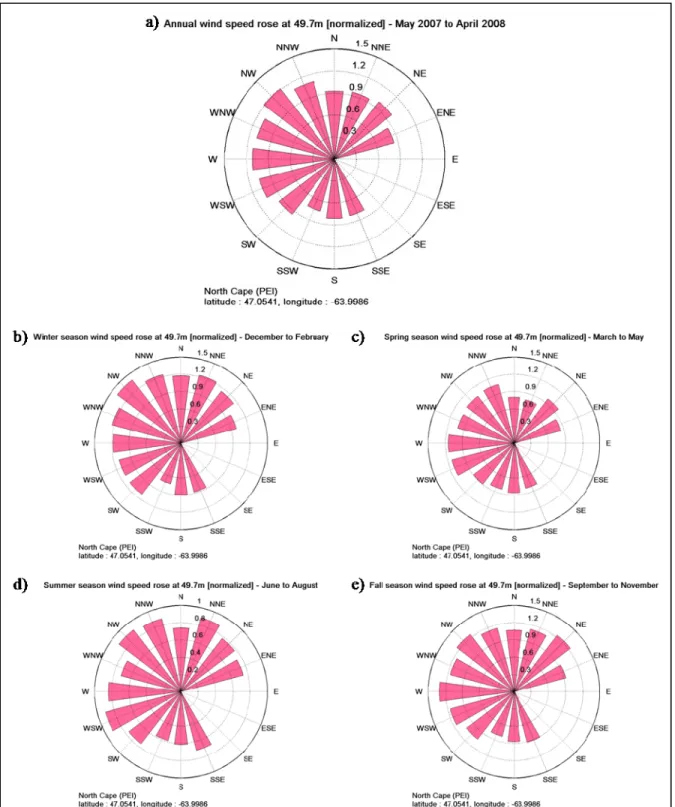
time lag. ...32 Figure 2.11 Annual and seasonal wind frequency roses at the North Cape site: a) annual,
b) winter, c) spring, d) summer and e) fall. ...34 Figure 2.12 Annual and seasonal average wind speed roses at the North Cape site:
a) annual, b) winter, c) spring, d) summer and e) fall. ...35 Figure 2.13 Annual and seasonal wind energy roses at the North Cape site: a) annual,
b) winter, c) spring, d) summer and e) fall. ...36 Figure 2.14 Annual and seasonal Weibull distributions of the wind speed at the North
Cape site: a) annual, b) winter, c) spring, d) summer and e) fall. ...37 Figure 2.15 Annual and seasonal average wind speed diurnal cycles at the North Cape
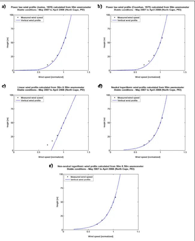
Figure 3.1 Vertical wind profiles under stable atmospheric conditions at the closest NWP point to the measurement mast (North Cape): a) Power Law profiles from Justus (1978), b) from Counihan (1975), c) linear profile, d) neutral and e) non-neutral logarithmic profiles. ...44 Figure 3.2 Vertical wind profiles under unstable/neutral atmospheric conditions at the
closest NWP point to the measurement mast (North Cape): a) Power Law profiles from Justus (1978), b) from Counihan (1975), c) linear profile,
d) neutral and e) non-neutral logarithmic profiles. ...45 Figure 3.3 Vertical wind profiles under stable atmospheric conditions at the closest
computation point with geographical characteristics similar to the site (North Cape): a) Power Law profiles from Justus (1978), b) from Counihan (1975), c) linear profile, d) neutral and e) non-neutral logarithmic profiles. ...46 Figure 3.4 Vertical wind profiles under unstable/neutral atmospheric conditions at the
closest computation NWP point with geographical characteristics similar to the site (North Cape): a) Power Law profiles from Justus (1978), b) from Counihan (1975), c) linear profile, d) neutral and e) non-neutral logarithmic profiles. ...47 Figure 3.5 Comparison of non-neutral logarithmic and linear profiles at the North Cape
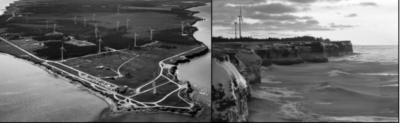
site. ...48 Figure 4.1 Photos of North Cape and the cliffs surrounding the wind test site. ...54 Figure 4.2 Plan of North Cape wind test site with part of the GEM-LAM horizontal
grid. ...55 Figure 4.3 Annual wind speed forecast RMSE rose for the North Cape site
(closest forecast point). ...56 Figure 5.1 Representation of the geographical parameters. ...59 Figure 5.2 Representation of the multilayer ANN architecture. ...68 Figure 5.3 ANN forecast RMS error for different parameters: a) number of nods,
b) learning rate and c) cross validation and momentum rate. ...71 Figure 5.4 Evolution of the performance of the a) D-MP linear and b) D-MP ANN. ...72 Figure 5.5 Measured annual wind frequency rose. ...72 Figure 5.6 Scatter plot of the measured and the forecasted wind speed
Figure 5.7 Wind speed forecast RMS error for different time series at the North Cape site: a) local time and b) forecast horizon (up to 48 h). ...77 Figure 5.8 Wind speed forecast RMS error for different meteorological parameters at
the North Cape site: a) wind speed, b) atmospheric stability (bulk
Richardson number), c) atmospheric pressure and d) air temperature. ...78 Figure 5.9 Wind speed forecast RMS error rose of each regression method at the North
Cape site: a) closest point, b) geo-referenced weighting, c) simple linear
regression, d) D-MP linear regression and e) D-MP ANN. ...79 Figure 5.10 Improvement rose of each regression module compared to the closest point
at the North Cape site: a) geo-referenced weighting, b) simple linear
regression, c) D-MP linear regression and d) D-MP ANN. ...80 Figure 6.1 Simple test cases on a) systematic, b) amplitude and c) phase errors. ...84 Figure 6.2 Legend for the NWP uncertainty assessment on amplitude and phase errors. ...86 Figure 6.3 a) Variation of the wind speed forecast error as a function of the time
window duration and b) autocorrelation function of the forecasted wind
speed. ...87 Figure 6.4 Wind speed forecast errors for different time series at the North Cape site:
a) local time and b) forecast horizon (up to 48 h)...90 Figure 6.5 Wind speed forecast errors for different meteorological conditions at the
North Cape site: a) wind speed, b) atmospheric stability (bulk Richardson number), c) atmospheric pressure and d) air temperature. ...91 Figure 6.6 Wind speed forecast error roses at the North Cape site: a) RMSE, b) phase
error, c) amplitude error and d) systematic errors. ...92 Figure 6.7 Wind speed forecast errors for dynamic meteorological events at the North
Cape site: a) pressure variations, b) temperature variations, c) wind speed variations and d) wind direction variations. ...93
ABBREVIATIONS AND ACRONYMS AGL Above ground level
ANN Artificial neural networks AST Atlantic standard time AVG Average
AWS Associated Weather Services CFD Computational fluid dynamics DISP Dispersion
E East MP Multi-point
D-MP Directional multi-point ENE East North East
ESE East South East
GEM Global environment multiscale model GMOS Geophysic model output statistic GMT Greenwich mean time
IEC International Electrotechnical Commission IREQ Hydro-Quebec’s Research Institute
LAM Limited area model LMS Least mean square MAE Mean absolute error MAX Maximum MIN Minimum
MLP Multilayer perceptron MOS Model output statistics
NB New Brunswick
NE North East
NN Nearest neighbour
NNE North North East NNW North North West
NSERC Natural Sciences and Engineering Research Council of Canada
NW North West
NWP Numerical weather prediction PEI Prince Edward Island
RMSE Root mean squared error S South
SDBias Difference between standard deviations
SE South East
SSE South South East SSW South South West STD Standard deviation
SW South West
USA United States of America W West
WEICan Wind Energy Institute of Canada WESNet Wind Energy Strategic Network WNW West North West
INTRODUCTION
Due to the global warming and to the many consequences of energy generation, industries and governments are promoting and developing power generation from renewable sources such as wind power. This type of energy has reduced impacts on the environment compared to more conventional power plants like nuclear, oil, natural gas and coal. As a matter of fact, in some European countries, up to 21 % of the energy generation comes from wind power (e.g. Portugal 9 %, Spain 12 % and Denmark 21 % (Global Wind Energy Council, 2008)) and this type of clean energy is also increasingly being adapted and used in North America.
One of the major concerns of integrating wind energy into electricity grids is the variability of the wind, and therefore, the power. With the sustained growth of wind energy installed capacity for electricity generation, electrical system operators need large amounts of spinning reserves from other energy sources to compensate for the fluctuations from the wind power, thus greatly affecting the cost of energy production. They also have increasing challenges optimizing the energy sources dispatch and minimizing the electrical network balancing costs. Therefore, wind power generation forecasting is an important issue for the economic efficiency of wind energy. More robust short-term (up to 48 hours) wind power forecasts will contribute to optimize the scheduling of conventional power plants and optimize the value of wind energy within the market in order to sustain the integration of wind energy in electricity portfolios of jurisdictions.
Three years of experimental meteorological forecasts in eastern Canada are available from Environment Canada Global Environment Multiscale Numerical Weather Prediction (NWP) model configured on a limited-area uniform 2.5 km horizontal grid spacing (GEM-LAM 2.5 km) for wind power predictions. These data also include forecasts for the region of North Cape on Prince Edward Island (PEI, Canada) where the Wind Energy Institute of Canada (WEICan) runs a test site for wind turbines and the PEI Energy Corporation operates a 10 MW wind farm. WEICan records wind speed at six different heights as well as wind direction, temperature and barometric pressure at single heights from a 60m mast, while the
PEI Energy Corporation records the total power production, the wind speed and the wind direction of each turbine at the same site. The forecasts, the power production and the atmospheric measurements use the same data format and the same time intervals (hourly averages), which facilitates model evaluation. With these two partners, it is thus possible to correlate model uncertainties to site characteristics or meteorological events and finally, to improve the forecast method itself.
The first chapter of this thesis gives a brief introduction of the state of the art on short-term wind forecasting and uncertainties, while an analysis of the database quality is performed in Chapter 2. Since data from different sources are available, a simple methodology is used to identify outliers. Data from both forecast and measured series associated to outlying data are removed in order to prevent errors due to outliers. Also, since vertical heat fluxes and temperature stratification have an impact on the vertical wind profile (see Chapter 1), low level thermal stability values derived from forecast outputs are integrated in the vertical interpolation of the wind speed to the anemometer height in order to improve the accuracy of this interpolation (Chapter 3).
In order to improve the Numerical Weather Predictions (NWP), a preliminary analysis over the North Cape site is conducted to define the parameters that shall be used to implement a Geophysic Model Output Statistics (GMOS) module (Chapter 4). The main objective of this research work is to improve short-term wind forecasting model by developing and applying different types of statistical modules (linear regressions, Artificial Neural Networks (ANN), etc.) to predict more precisely the wind speed as a function of the site characteristics and meteorological parameters (Chapter 5). Statistical techniques have been preferred over physical micro-scale models as they are computationally inexpensive (see Chapter 1). Calibration of the GMOS is done using one year of data and then, the evaluation phase takes place over the remaining period. Note that, in order to generalize the results, a validation of the complete methodology is also performed using a similar meteorological tower owned by Université de Moncton which is located in Bouctouche (New Brunswick (NB), Canada).
Throughout this work, in order to express the forecast error characteristics, many statistical criteria and error indicators are computed while figures and graphs are produced to illustrate the different results. Mainly, the mean absolute error (MAE) evaluates the error directly in terms of wind speed prediction; the root mean squared error (RMSE) evaluates the error in terms of wind speed prediction and verifies the error distribution; the bias evaluates the systematic error. Note that the standard deviation (STD), being a component of the RMSE, can also be used to verify the error distribution, but as the RMSE will be decomposed in Chapter 6 to represent different characteristics of the forecast errors, this criteria is preferred over the STD. In all cases, these criteria are normalized with the site annual mean wind speed to maintain the results independent from the site itself. Furthermore, to compare different models, an improvement indicator is also used. The final section of this thesis (Chapter 6) presents the analysis of the short-term wind forecasts uncertainties. This expanded work is done using amplitude and phase error description as well as exploratory analyses to detail the uncertainty characteristics and different error tendencies or evolution in time. This analysis is used as a dynamic approach to evaluate the contribution of meteorological events to forecast errors; meteorological situations related to high uncertainty of short-term wind predictions can then be identified.
The objective of the current study is to optimize the use of short-term NWP for complex sites by applying statistical methods. The conclusions of this assessment contribute to the development of the forecast model with Environment Canada by applying the GMOS developed and notably by identifying meteorological events with high uncertainties by means of the evaluation protocol being developed. Ultimately, a better knowledge of these uncertainties and better wind forecasts will increase the economic value of wind energy in the market.
CHAPTER 1 LITERATURE REVIEW
1.1 Numerical wind power prediction models
Landberg et al. (2003) and Giebel et al. (2003) provide complete reviews of wind power prediction models. They show that most short-term wind power forecast models use the available regional NWP as input parameters, usually geostrophic wind speed and direction. Generally, those NWP models have a coarse spatial resolution ranging from 5 to 25 km. Therefore, the first step in wind power predictions is to estimate the wind resources at the exact wind farm location (wind speed and direction). This downscaling operation is generally done using a physical Limited Area Model (LAM) with higher resolution (meso-scale or micro-(meso-scale) and employing the global NWP as initial lateral boundary conditions. Also, high resolution topography and surface roughness measurements are used to characterize the site.
Then the wind speed at the site is generally scaled down to the turbine rotor height by applying a logarithmic vertical profile for neutral atmospheric stability. Landberg (1998) shows that it is also possible to correlate the geostrophic wind with the surface wind by using a simple relation, assuming the geostrophic drag law as a linear function. Considering different surface roughness, along with the geostrophic wind speed and direction, he points out that it is possible to predict surface wind speed directly from the geostrophic wind under neutral atmosphere. He also demonstrates that the variation in the wind direction with height (Ekman spiral) is one of the most difficult parameter to predict and cannot be simplified into a simple relation. Nonetheless, wind speed can be predicted using simple methods with a relatively good accuracy (in comparison with micro-scale models). Finally, correlations are generally developed using the turbine power curves to convert the surface wind to electrical power. The wind power forecast models can also take into account the wind farm layout to integrate the wake effect of a turbine on the aerodynamics of the whole wind farm into the final wind power forecast.
1.2 Model output statistics
Most wind power prediction models use Model Output Statistics (MOS) to correct biases and the general amplitude errors (auto-regressive statistical models, ANN, etc.). When used off-line, MOS are calibrated using historical wind farm data in order to search for the optimal statistical parameters. If the power production data are available online, MOS can be calibrated in real time. Therefore, online data offer many advantages. Tuning off-line MOS needs considerable efforts compared to self calibrating MOS; online MOS adapts themselves to annual and seasonal variations, farm layout and data quality. Also, Kariniotakis et al (2004) show that Kalman filtering techniques clearly improve NWP systematic errors for linear (e.g. temperature) and non-linear parameters (e.g. wind speed). Since statistical techniques are computationally inexpensive, they conclude that it is worthwhile using them. With a proper MOS, systematic errors remain low. Thus, there remain two types of random errors still occurring in wind power forecast: amplitude and phase errors. The amplitude error misjudges the intensity of a meteorological event and the phase error misplaces the event in time. Therefore, since the wind power forecast is affected by both the intensity and occurrence of the wind, work is needed to assess the uncertainties of models on the amplitude and the phase errors of wind speed forecasts.
1.3 Reference models
When comparing different NWP models to obtain their performance evaluation, it is interesting to first define a reference model using only simple physical considerations (Madsen et al., 2004). Ten years ago, persistence models, where the future wind is assumed to be the same as the last measured wind speed, along with climatology predictions, using the annual mean wind speed, were used as reference models. These basic models were used for their simplicity and because persistence is excellent for short-term forecasts up to 3 - 6 hours (Landberg and Watson, 1994; Liu, 2009). This is explained by the fact that the atmospheric motion is driven by pressures systems which changes much more slowly than wind turbulence, since the time scale of pressures systems is in the order of days.
More recently, Nielsen et al. (1998, p. 29) defined a new reference model because they found that “it is not reasonable to use the persistence model when the forecast length is more than a few hours.” Thus, they merged both the persistence and the climatology prediction models. To get the new reference model, they linearly combine the old reference models for each forecast horizon. This new model performs better than both individual models for all time horizons. Since then, this new reference model is used to compare the different NWP models being analyzed for different time horizons. Note that the new reference model has to be calibrated with measured time series to determine the statistical parameters using the autocorrelation of the wind speed from measured time series (Madsen et al., 2004). Therefore, it is important to split the database and clearly define the calibration data (as for any learning model) and the test data for the error analysis. Then the performance evaluation of the model has to be done with the test data.
1.4 Performance evaluation of models
Before carrying out the performance evaluation with different criteria, it is important to verify the quality of the data. One can perform a visual check of the data to ensure that there are no outliers within the data (e.g., zero wind speed due to icing of an anemometer) or, if data are available from different measurements, they can be compared directly to identify the outliers. Kariniotakis et al. (2004) also points out that it is necessary to use common data (NWP, power production and atmospheric measurements) and common data format for proper model comparison. Then, in the standardized protocol for performance evaluation of prediction models (Madsen et al., 2004), a guideline is presented to properly use statistical criteria to determine the power prediction uncertainties. It is recommended using many statistical criteria, to express different error characteristics.
In order to evaluate the errors directly in terms of amplitude, it is recommended to use the MAE, while the STD is used to evaluate the error distribution to get the confidence interval based on the Gaussian distribution. Note that larger absolute errors have larger effects on the RMSE than on the MAE. Therefore, when used along with the MAE, the RMSE can be used
to obtain details on the error distribution. The bias can still be computed to verify the systematic error, since there is no perfect MOS. In all cases, it is important to normalize these criteria with the installed power capacity of the wind farm or the mean wind speed. This operation makes the results independent from the wind farm or the site itself. When the objective is to compare prediction models, it is recommended to use the improvement criterion, also referred to as “skill” score. This criterion is defined as the difference between the error of the reference model ( ) and the analyzed model error ( ), normalized with the reference model error ( ).
∞, 1 (1.1)
The improvement can be computed for each of the criteria presented above. An improvement score of zero means that the model performs as well as the reference model. Conversely, a perfect model would get a score of one; while a negative score means that the reference model performs better than the analyzed model.
Madsen et al. (2004) also recommend the use of exploratory analyses to detail the uncertainty analysis. A histogram plot or a cumulative squared error graph can help to illustrate different error tendencies or evolution in time. These analyses can point out a time period that needs further investigations (due to changes in the NWP). Kariniotakis et al. (2004) use the forecast with errors lower than 10% to visually compare the analyzed models in a graph. They also use the minimum and maximum values of the errors as exploratory analyses to characterize the model uncertainties. The general results of the performance evaluations need to be expressed for a precise time horizon (generally 6 or 12 h), for some time periods (seasonal) or for meteorological events.
1.5 Benefit of ensemble forecasts
It is well known that the accuracy of the NWP models is a major concern in wind power predictions. Doubling the spatial and temporal resolution of the NWP models would increase the computational time by a factor of at least eight. But the exact same computational time could be used to run an ensemble of eight members (combining different NWP models) in order to obtain a better forecast. A solution to this problem is to use NWP ensembles to significantly reduce the RMSE. It is shown that a combination of an ensemble of predictions outperforms the individual NWP members (Lange et al., 2006) and ensemble forecasts can also give the confidence level of the predictions. Such combination is done by statistically weighting the NWP for different weather classes. Ensemble forecast can be achieved either by using different NWP models, by using different parameterization of the same model or by varying the input data (Nielsen et al. 2004 and Nielsen et al. 2007a).
Nielsen et al. (2007a) point out that the operational robustness (reliability or accuracy) of a model is highly increased by using data from different sources. Nielsen et al. (2004) also achieve ensemble forecasts using different parameterization of the same model or by using perturbed initial conditions. Statistical methods combining the NWP and the new reference model is another way to get sophisticated bias correction (e.g. Wind Power Prediction Tool model). Based on a combination of the different forecast properties (variance, kurtosis, skewness, etc.) and the weather conditions, with low linear correlation between the different members, ensemble forecast almost guarantee improvements of the model (Nielsen et al., 2007b). In this work, it is also recommended to realize ensemble forecast using only few good uncorrelated forecasts, rather than a multitude of correlated forecasts. The statistical weighting and bias correction of the ensemble forecast can be computed using error, variance or meteorological characteristics criteria. Like MOS, ensemble forecast models tend to give better results (lower MAE and higher correlation) with regular recalibration or online auto-calibration (Nielsen et al., 2007b).
1.6 Challenges to overcome
In most wind farm applications, the end users (wind farm managers, transmission system operators, energy service suppliers and traders) are not the ones who run the NWP models; rather, they only use the predictions. The end users experience directly the consequences of the forecast errors, such as the variation in the price of energy on the market, supply contracts, operating costs and security concerns. Therefore, it is important to provide an appropriate estimate of the forecast error.
Many studies show that it is difficult to forecast sudden and pronounced changes in the weather produced by meteorological events such as the passage of a meso-scale front. For instances, Lange and Heinemann (2003) show that forecast errors are highly related to the local meteorological events. Days with typical meteorological conditions can be classified using synoptic meteorology (historical data including pressure as well as wind speed and direction). They use one average error value per day to compare the different groups and they find a profound difference within different weather situations. Dynamic events, like low pressure systems, produce much higher forecast uncertainties than quasi static ones, such as high pressure systems. Cutler et al. (2007) have similar conclusions about wind power ramps (high phase and amplitude errors).
Kariniotakis et al. (2004) point out an important diurnal variations of the MAE for some European NWP models, indicating that there is still a lot of work to do to integrate surface heat fluxes (Landberg and Watson, 1994) and temperature stratification (Lange and Heinemann, 2003) in these models. These phenomena related to atmospheric stability are still quite difficult to predict. Similarly, Kariniotakis et al. (2004) observe that model uncertainties are directly related to the terrain complexity. In another study, Nielsen et al. (2007a) show that using planetary boundary layer stability measures derived from meteorological forecasts improves the forecast for complex sites. These results suggest including some physical parameters (atmospheric stability or terrain characteristics) in MOS to get more accurate predictions, especially for sudden meteorological events.
Subsequently, according to the needs of electrical systems operators, the objective of the present study is to develop a GMOS which integrates terrain and wind characteristics to improve the wind forecast of a NWP model, particularly in complex terrain. Also, it is intended to integrate stability as derived from meteorological forecast in the vertical interpolation of the wind speed forecast. The purpose of these assessments is to contribute to the development of the forecast model used at Environment Canada by applying such techniques and notably by identifying meteorological events with high uncertainties by means of an evaluation protocol. Finally, phase, amplitude and systematic errors decomposition intend to help defining NWP research priorities in improving wind energy forecasting.
CHAPTER 2 MEASUREMENT DATA
At the North Cape site, the WEICan records wind speed at six different heights as well as wind direction, temperature and barometric pressure using a mast located at 47.054082 N, 63.99865 W (see Figure 2.1). Except for the atmospheric pressure, the exact same data is gathered at the Bouctouche tower located at 46.472217 N, 64.73915 W (see Figure 2.2). These 60 m towers have respectively a 0.3 m (triangular lattice tower) and 0.152 m (tubular tower) width. Figures 2.1 - 2.2 present the location of both sites: the cross represents the anemometer tower while the grid represents a subset of the Environment Canada GEM-LAM horizontal grid for wind predictions. Tables 2.1 - 2.2 present the different sensor types and their configuration on both towers.
Figure 2.2 Bouctouche site location (NB, Canada).
Table 2.1 Sensor descriptions and positioning on the North Cape anemometer tower
# Sensor model Height (m) Boom length (m) Orientation (°)
N1 NRG Type 40 Maximum Anemometer 9.83 0.89 295
N2 NRG Type 40 Maximum Anemometer 16.95 0.97 295
N3 NRG Type 40 Maximum Anemometer 26.96 1.02 295
N4 NRG Type 40 Maximum Anemometer 39.79 1.06 295
N5 Barometric Pressure Sensor 61205V 41.50 - -
N6 NRG 200 Series Wind Vane 48.82 0.83 55
N7 Campbell Scientific Temperature Probe-107/108
49.22 - -
N8 NRG Type 40 Maximum Anemometer 49.70 1.32 295
N9 NRG Type 40 Maximum Anemometer 58.37 1.44 295
Note that the atmospheric measurements (10 minute averages and STD from 1Hz data), along with the forecasts, use the same data format and the same time intervals which allows proper model evaluation. It is important to note that the first year of the measurement data is
used to train the different statistical modules that are implemented for both sites (Chapter 5). Then, for the evaluation phase (Chapter 6), it is suggested to use at least eight month of data (one complete year is recommended) in order to produce results that are representative of the model behaviour in an actual wind power plant, which operates all year around. This recommendation is based on the fact that model evaluation over shorter period than eight months shows non representative results: insufficient evaluation data put emphasis on a certain season, which is not desirable when assessing the evaluation of the general performance of a model. Yet, two complete years of data (May 2007 to April 2009) are available for the North Cape site, but only 22 month of data (July 2008 to April 2010) are available for the Bouctouche site. Therefore, the first year of both time series is used for the training phase and the remaining period is set as the validation database.
Table 2.2 Sensor descriptions and positioning on the Bouctouche anemometer tower
# Sensor model Height (m) Boom length (m) Orientation (°)
B1 NRG Type 40 Maximum Anemometer 10.0 1.5 315
B2 Campbell Scientific Temperature Probe 107/108
3.0 - -
B3 NRG Type 40 Maximum Anemometer 30.0 1.5 315
B4 NRG Type 40 Maximum Anemometer 40.0 1.5 315
B5 NRG Type 40 Maximum Anemometer 50.0 1.5 315
B6 NRG 200 Series Wind Vane 58.0 1.5 345
B7 NRG Type 40 Maximum Anemometer 60.0 1.5 315
B8 NRG Type 40 Maximum Anemometer 60.2 1.5 135
With the training and validation databases set for both sites, it is now possible to perform the data quality analysis. Since measurements from different sensors are available, a simple methodology is used in section 2.1 to identify outliers. Then, in section 2.2, an analysis is performed to select the appropriate anemometers that have to be used to test and validate the NWP model. In Tables 2.1 - 2.2, it is possible to note that every sensor is mounted no closer
than 1.5 times the tower width to avoid high flow distortion due to the mast (Kaimal, 1994) which is analyzed in detail in section 2.3. Thus, a complete analysis of the measurements uncertainty is conducted to verify that the database is suited for the NWP model evaluation. Finally, section 2.4 presents the wind characteristics on the sites.
2.1 Data quality analysis
Before processing the data and assessing any model validation, it is essential to analyse the quality of the data sets. Following the data validation methodology proposed by the Associate Weather Services (AWS) Scientific (1997), a computer based routine is coded to automatically identify suspect values. Then a case-by-case verification is done to ensure that only erroneous values are removed from the database, permitting a high data recovery rate. The validation procedure, illustrated in Figure 2.3, is grouped in three different categories: data sequence checks, measured parameter checks and data treatment. The data sequence check is done to ensure that the records are complete. Verifying the number of records for each parameter compared to the time series allows to find missing sequential values. In fact, for the North Cape site, some icing events and some electrical failure are already indicated in the files by WEICan and hourly data are removed. This first check indicates the total number of record available for the analysis among the raw data.
Subsequently, it is possible to verify the records of each measured parameters. Since a single criterion is unlikely to detect every problematic situation, three different types of test are used to identify outliers. A range test is used to ensure that all collected data are logged into physical value ranges: there should not be any negative values (except for the temperature); usual sensor calibration gives an offset value of 0 or 0.035 m/s for zero wind speed; measured values should not exceed a reasonable range of values, such as 30 m/s average speed and 40 m/s maximum gust speed for example.
On the other hand, since data are available from different sensors, a relational test is also performed to compare the output of the anemometers located on the same tower. This relational test allows verifying that the sensors represent an appropriate vertical profile of the wind. Note that the North Cape site is surrounded on the East, North and West sides by a coastal cliff which has an average height of 13 m (see Chapter 3). Gasset et al. (2005) have shown that such a cliff affect the wind speed near the ground up to a distance of ten times the cliff’s height. Even though the tower is further than 130 m away from the cliffs, sensors #1N and #2N have not been used in this study because the turbulent kinetic energy of the flow still appears to be influenced by the cliff in this area up to twice the cliff’s height above ground level (AGL) (Gasset et al., 2005). Similarly, the Bouctouche site is surrounded by a forest canopy; therefore, for the same reasons, the 10 m anemometer on Bouctouche mast (#1B) is not used.
The last check, the trend check, verifies if the temporal variation of a measured parameter exceeds the usual physical behaviour due to the inertia of the atmospheric system. The validation criteria proposed by AWS Scientific (1997) for sites located in the United States of America (USA) are not used in this study due to differences in climate regime between USA and Canada. Instead, “normal fluctuation” ranges are determined according to the eastern Canadian climate, which is consistent with the measurements. The validation criteria that are used for the Canadian sites are listed in Tables 2.3 - 2.5. Note that a violation of one of these criteria flags the data as suspect. Afterward, all identified events are verified case-by-case to ensure that only erroneous values are removed from the database.
Table 2.3 Sensor range test criteria for the eastern Canadian climate
Parameter type Sample parameter (10 min) Validation criteria
Wind speed Average 0.035 < AVG < 30 m/s Standard deviation 0 < STD < 4 m/s
STD = 0 only if AVG = 0.035 m/s Maximum & minimum gust 0.035 < MIN or MAX < 40 m/s Barometric pressure Average 96 < AVG < 104 kPa
Wind direction Average 0 ≤ AVG < 360 ° Standard deviation 0 < STD < 90 °
STD = 0 only if AVG < 5 m/s Temperature Average -25 < AVG < 35 °C
Table 2.4 Sensor relational test criteria for the eastern Canadian climate
Parameter type Sample parameter (10 min) Validation criteria
Average wind speed 30 m / 40 m difference ≤ 2 m/s 30 m / 50 m difference ≤ 2.5 m/s 30 m / 60 m difference ≤ 3 m/s 40 m / 50 m difference ≤ 2 m/s 40 m / 60 m difference ≤ 2.5 m/s 50 m / 60 m difference ≤ 2 m/s Maximum wind gust speed 30 m / 40 m difference ≤ 5 m/s 30 m / 50 m difference ≤ 5 m/s 30 m / 60 m difference ≤ 5 m/s 40 m / 50 m difference ≤ 5 m/s 40 m / 60 m difference ≤ 5 m/s 50 m / 60 m difference ≤ 5 m/s
Table 2.5 Sensor trend test criteria for the eastern Canadian climate
Parameter type Sample parameter (10 min) Validation criteria
Average wind speed Mean variation ≤ 10 m/s within 1 h Average temperature Mean variation ≤ 7 °C within 1 h
Sign change ≤ 2 within 3 h
Only if daily AVG < 3°C Average barometric pressure Mean variation ≤ 1.5 kPa within 3 h
Once the validation methodology is applied, the case by case verification show that the measured parameter checks point to suspicious data (Figures 2.4 – 2.7). Figure 2.4 shows an event (North Cape, February 27th, 2008) where wind data is removed from the database due to the icing of the anemometers. Looking at the temperature profile which is slightly under the freezing point and looking at the wind vane that has a constant direction with no variation (STD equal to zero); it is very likely that there was effectively an icing event. All parameters show regular fluctuations within the day but the wind speed and direction are not valid from 10:00 AM; the wind speed has been removed from the database and the wind vane was iced in the North-East direction. Since the wind speed was over 10 m/s before the icing event, the icing of the anemometer causes an artificial decreasing trend in the wind speed which is detected by the validation methodology. Also, the method identifies high variations of the wind speed caused by malfunctioning sensors or created artificially by missing data. In almost all cases, the verification of the data associated with suspicious wind ramps (identified by the method) showed an abnormal behaviour of the sensors. Overall, only one normal wind increase is pointed out as suspect data: this event is therefore reincorporated in the database and all erroneous data (e.g. the event showed in Figure 2.4) are removed.
Furthermore, applying the same data validation methodology, another type of suspect data where some maximum wind speeds are recorded to a peaking value over 1 000 m/s is being pointed out repeatedly. Because of these abnormal wind gusts, the STD of the wind speed also reaches an extremely large value. The mean wind speed is also found to be abnormally
large. The mean wind speed and STD, as well as the average wind direction and STD, for one irregular event can be observed in Figure 2.5. Monitoring the graphs of Figure 2.5, one can see that the identified time series (North Cape, June 25th, 2007) contain three aberrant data which do not represent properly the physical behaviour of the wind speed between 13:00 and 18:00. It can also be observed that there is a high wind direction STD as the wind direction changes suddenly and repeatedly during this event. This might show a dynamic meteorological event occurring that day, but there is no low pressure system that could explain such large change in wind speed. The temperature is above zero which confirms that there is no icing event. The 60 m anemometer records extremely high wind gust which are abnormal. This implies that there is an electrical issue with the sensor: the electrical output does not always match the input wind speed. Again, these observations show that the methodology used to remove data from malfunctioning anemometers is proper and those outlying data are removed from the database.
This verification also shows that the computer based methodology is able to point out irregular behaviour of the atmospheric boundary layer wind profile. Figure 2.6 shows an event (North Cape, June 4th, 2007) where the measured wind speeds are not following a regular vertical profile: greater wind speed at higher measurement locations should be observed. It is important to note that, because of the turbulent nature of the wind, it is possible to observe short moments (up to few hours) where the wind does not follow this profile, but this phenomenon should not be observed for long time period. For a period longer than 6 h during that day (from 15:00 to 22:00), the averaged wind speeds are following a non physical profile (i.e. lower wind speeds measured by the 60 m anemometer) due to a malfunctioning anemometer. Consequently, all situations of irregular vertical profile of the wind speed found by the methodology are removed to assure data quality.
Finally, some other erroneous data are found to be suspect. Figure 2.7 shows an event (North Cape, June 6th, 2007) where the pressure and temperature sensors are malfunctioning between 14:00 and 15:00. Normally, temperature and pressure are parameters that have a
Figure 2.4 Time series of a suspect icing event: a) air temperature, b) barometric pressure, c) average wind speed, d) maximum wind speed,
Figure 2.5 Time series of suspect wind gusts: a) air temperature, b) barometric pressure, c) average wind speed, d) maximum wind speed,
high inertia and change slowly in time: these variables shall not fluctuate suddenly nor shall they venture out of certain physical limits. During this event, the pressure sensor suddenly drops down to 10 kPa as the temperature sensor measures -90°C while all other sensors seem to function properly. Such fluctuations are not physically possible and many events (~ 12/year) similar to this particular one are identified within the database. This method allows removing those erroneous data.
Figure 2.6 Time series of a suspect vertical wind profile: average wind speed.
Ultimately, the main parameters (temperature, pressure, wind speed and direction) are plotted over the complete time series. This final visual check done on the entire time series of each parameter allows to quickly validate that all evident erroneous data are found by the methodology. The complete verification shows that the method has been able to identify many types of erroneous values. Only few normal events are recognized as suspect data, but with the case-by-case verification, they have been kept in the database. These verifications induce a high data recovery rate while minimizing the risk of keeping erroneous values. Two complete hours of data is removed for every event (one before and one after) to ensure that the sensors are fully functional due to the inertia of some events, like icing.
Moreover, as mentioned earlier, locating the anemometer on a boom at least 1.5 times longer than the tower width generally protects the instruments from the disturbed flow due to the tower, but it does not keep the sensors away from tower shadowing. In fact, the tower shades the sensor and reduces the downwind wind speed significantly (Hunter et al., 1999). This effect mainly covers a downwind angle of 30° on both sides of the tower for a total angle of 60° where the data should be excluded (Kaimal, 1994). For the same positioning, a wind vane suffers a maximum deflection of 5° due to tower shadowing (Kaimal, 1994), but since the wind directions are binned into 16 sectors of 22.5° each, such deflection does not affect much the binned value of the wind direction. Subsequently, records when the anemometers are located downwind to the tower are removed from the database (i.e. E, ESE and SE directions for the North Cape site and ESE, SE and SSE directions for the Bouctouche site).
Furthermore, as the NWP model is set for output at hourly time steps representing the instantaneous average wind speed, the last 10 min measurements of each hour is used to describe the average wind speed at the same time stamp (see section 2.3 for a description of temporal averages). Subsequently, for a single outlying datum within the measurement database, data from both the forecast and the measured series associated to the same time period are removed in order to compare identical databases. Note that before using any onsite measurements, it is essential to offset the forecast time series since the predictions are done using the Greenwich Mean Time (GMT) zone while the measurements are acquired on
the Atlantic Standard Time format (AST = GMT-4). Finally, according to the following equations, the data recovery rate is calculated using the total possible records, with the number of available records and available forecast records included in the database as well as the number of invalid records and the number of shadowed records that are removed:
100 (2.1) 100 (2.2) (2.3) 1 100 (2.4) 100 (2.5) 100 (2.6)
Table 2.6 presents monthly and annual results for each of the parameters that are previously computed using two years of data from North Cape. The results for Bouctouche site are quite similar and they are shown in the annexes (see Annex I: Table A.I.1). These tables show that many measurement data are not available during the cold season (January to March), mainly due to icing of the instruments. Also, it is possible to observe that the data validation methodology removed many data from the database from December to March also due to the high occurrence icing events. In addition, this methodology removed a significant number of data during the months of May, June and July because the North Cape 60 m anemometer did experience electrical problems as mentioned earlier (i.e. high measured gust speeds). Data have also been removed downwind of the tower to avoid measurements
suffering from shadowing and the number of data removed depends on the wind frequency for the given wind direction of each month. As the instruments are purposely installed on the most frequent upwind direction, the number of downwind data removed is relatively low. On the other hand, the available forecast ratio does not rely on any environmental variables; it depends on the computational capability to run the model. Since it is an experimental forecast for the wind energy sector, Environment Canada operational forecast always prevails. Therefore, these forecasts have been executed on a dedicated cluster located at Hydro-Quebec’s Research Institute (IREQ) and this is the reason why the available forecast ratio is 100% (not in real time). Finally, the total data recovery rate related to the present study is 78.84%. This amount of data is sufficient for the purpose of validating a forecast model.
Table 2.6 Data recovery rates for every month of the sample year (North Cape)
Month Available Records Ratio (%) Valid Records Ratio (%) Shadow Free Records Ratio (%) Available Forecast Ratio (%) Data Recovery Rate (%) January 95.36 88.23 95.37 100.0 80.24 February 95.61 80.20 89.61 100.0 68.71 March 89.52 84.98 92.23 100.0 70.16 April 97.50 87.39 88.92 100.0 75.76 May 99.80 87.47 86.14 100.0 75.20 June 99.86 91.31 78.83 100.0 71.88 July 99.80 91.72 92.07 100.0 84.28 August 100.0 95.90 83.18 100.0 79.77 September 100.0 94.44 92.13 100.0 87.01 October 98.92 94.02 93.35 100.0 86.82 November 100.0 94.51 86.99 100.0 82.21 December 100.0 92.20 91.11 100.0 84.00 Annual 98.03 90.20 89.16 100.0 78.84
2.2 Anemometer selection
As a measurement mast presents many anemometers, one of them is selected to be compared with the NWP model outputs for model validation. This is the reason why four different logarithmic vertical wind profiles are plotted and the surface roughness is computed for the entire time series of the mean wind speed. The wind profiles are shown in Figure 2.8 and Tables 2.7 - 2.8 details the computed surface roughness. Similar wind profiles are found for the Bouctouche site in the annexes (see Annex II: Figure A.II.1). All parameters are computed from a neutral logarithmic equation comparing the wind speed at two different heights to interpolate the average wind speed to another location using equations 2.7 - 2.10. Note that the surface roughness describes the height where the wind speed is zero. This length is generally used in meteorology to define the ground surface and the obstacles on site. It is possible to compute the surface roughness (z ) and the surface friction velocity (u ) using wind speeds at two different heights:
/ (2.7)
/ (2.8)
(2.9)
/ / / (2.10)
Where: U z is the interpolated wind speed [m/s] at height z [m];
- U and U are the measured wind speed [m/s] at heights z and z , respectively [m]; - k is the Von Karman similarity constant (0.4 [-]);
Figure 2.8 Logarithmic vertical wind speed profiles plotted from the mean wind speed at two different heights.
Table 2.7 Surface roughness computed from the mean wind speed at different heights (North Cape)
Anemometer height Surface roughness on site ( ) 49.70 m & 58.37 m 0.7033 m 39.79 m & 49.70 m 0.1362 m 26.96 m & 39.79 m 0.3335 m 26.96 m & 49.70 m 0.2552 m 26.96 m & 58.37 m 0.3180 m 39.79 m & 58.37 m 0.3002 m
Table 2.8 Surface roughness computed from the mean wind speed at different heights (Bouctouche)
Anemometer height Surface roughness on site ( ) 50 m & 60 m 1.9453 m 40 m & 50 m 4.2256 m 30 m & 40 m 3.4345 m 30 m & 50 m 3.7352 m 30 m & 60 m 3.3252 m 40 m & 60 m 3.2239 m
Subsequently, the comparison between the different logarithmic profiles derived from the annual average wind speed of each anemometer on the same tower (Figure 2.8) shows that the 50 m anemometer operates very close to all calculated profiles for the measurement period at both sites. Also, looking at Table 2.7, one can notice that the only set of anemometers giving a representative surface roughness for North Cape site is using the 30 m and the 50 m (i.e. surface roughness for a fallow field with many small wind turbines and few small buildings shall be slightly higher than 0.25 m (Manwell et al., 2002)). However, when assessing a wind power monitoring program, it is important to use the highest sensor as possible to be relatively close to current standard turbine hub heights. The quality control of the data shows that the 60 m anemometer often reads maximum wind gust speeds that are not physically possible. Therefore, the second option would be to choose the 50m anemometer which is working as predicted by the different logarithmic profiles and which gives a surface roughness value representative of the site characteristics. In addition, the two first NWP output levels are given for different pressure levels and are located relatively close to 45 m and 120 m above ground. These are sufficient reasons to choose the 50m sensor which is very close to the first level of the forecast model, while being very close to the wind vane, the temperature probe and the barometric pressure sensor that are also located between 40 and 50 m high. For these reasons, the sensor #8N (NRG Type 40 Maximum Anemometer, 49.7 m) is chosen to details the wind characteristics for the North Cape site.
The same methodology applied to the anemometers mounted on the Bouctouche mast lead to choose the sensor #5B (NRG Type 40 Maximum Anemometer, 50 m high) for the validation of the Environment Canada NWP model. It is also interesting to note that, looking at Table 2.8, the roughness length computed for the Bouctouche site is approximately 3.5 m. Such roughness length is generally associated to urban areas with very large buildings, which is not the case here. This site is actually surrounded by a forest canopy which has a roughness length of about 1.5 m (Manwell et al., 2002) as used in the inputs of the NWP model. Stull (1988) explains that a dense forest canopy could act like a displaced surface of height “d” (see Figure 2.9), which is not considered in the NWP model. Therefore, one shall expect that the wind speed forecast error is higher for the Bouctouche site than the North Cape site.
Figure 2.9 Vertical wind speed profiles over forest canopy. (adapted from Stull, 1988, p. 381)
2.3 Atmospheric measurement uncertainty
Now that the anemometers have been chosen and that all erroneous values have been removed from the database, the measurement uncertainties can be computed in order to verify that the measurement dataset is well suited to evaluate the model. It is known that cup anemometer precision is of the order of 3 % (AWS Scientific, 1997), but it is also important to compute the wind speed deficit due to the flow distortion around the anemometer tower (excluding shading area) and the precision of the averaging technique.
First, the flow distortion in the surrounding area of the tower can be computed using the geometrical and conception parameters of the triangular lattice tower (IEC, 1998):
100% 1 0,062 0,076 0,082 (2.11)
2,1 1 (2.12)
Where: U is the wind speed deficit [%]; - CT is the drag coefficient [-];
- t is the solidity of the tower (0.1 < t < 0.3); - R is the distance to the mast centre [m]; - L is the mast leg distance (0.6025 [m]).
The distance to the mast center (R) can then be expressed as a function of the mast leg distance (L) and the boom length (BN C 1.32 m) for a triangular lattice mast:
tan 30° (2.13)
As the anemometer tower solidity is not known, the highest recommended value is used in order to be conservative. Then, for the Bouctouche tubular mast, the wind speed deficit is computed as a function of distance (d 1.5 m) from the centre of a tubular mast and mast diameter (d 0.152 m). The relation is given in the IEC standard (1998) from a two dimensional Navier-Stokes analysis. Subsequently, the average centreline wind speed distortion is approximately 1.3 % for the North Cape tower and 0.1 % for the Bouctouche tower.
Afterwards, when characterizing experimentally a turbulent flow, the averaging technique precision shall be computed since measurements are usually averaged over many realizations
under similar conditions (i.e. ensemble averaging). In the atmospheric boundary layer, due to the stochastic behaviour of the turbulent flow, it is almost impossible to observe identical events and to perform ensemble averaging. Then, when describing the properties of the atmospheric air flow, data are averaged over time. Time averages are performed considering that they are equivalent to ensemble averages. This assumption is called the ergodic hypothesis (Lumley and Panofsky, 1964).
The atmosphere is also assumed to be statistically stationary during the averaging period (Tennekes and Lumley, 1972). Van Der Hoven (1957) shows that there is a gap between convection driven boundary layer scales (shorter than 0.001 Hz ~ 16.67 min) and synoptic scales (greater than 0.0001 Hz ~ 2.78 h) where the spectral intensity is negligible. Consequently, the atmosphere fluctuations can be assumed to be stationary for averaging period shorter than the convection driven scales (i.e. 10 min averages). Thus, considering that high frequency component of the wind, as turbulent wind gusts, have no significant contribution (zero average) in the mean meteorological phenomena. Conversely, when computing time averages, it is important to average over a sufficiently long sampling time (Panofsky and Dutton, 1983): this allows to properly describe the mean wind speed and limiting the statistical influence of the autocorrelation of the turbulence. Since the surface wind speed measurements are used for the NWP model validation, it is therefore important to estimate the error due to finite integration time.
When performing time averages, a common approach used in meteorology to express any parameter is to decompose each and every variable into a mean part and a perturbation part (Taylor’s hypothesis). In equation 2.14, the perturbation or turbulent part (U ) superimposed on the average part (U) represents the instantaneous value (U) (Stull, 1988). These fluctuations are computed in the NWP model but are not commonly used as model outputs. For this reason, no distinction is made between mean or instantaneous parts after the present section since this study is only based on mean variable outputs. Therefore, in the rest of the document, for notational simplicity, this bar representing the average part of a variable will not be specified anymore.