Optimisation du design des réseaux de surveillance de la qualité de l'eau en maximisant la valeur économique de l'information

(1)

HAL Id: tel-03139960

https://tel.archives-ouvertes.fr/tel-03139960

Submitted on 12 Feb 2021

HAL is a multi-disciplinary open access archive for the deposit and dissemination of sci-entific research documents, whether they are pub-lished or not. The documents may come from teaching and research institutions in France or abroad, or from public or private research centers.

L’archive ouverte pluridisciplinaire HAL, est destinée au dépôt et à la diffusion de documents scientifiques de niveau recherche, publiés ou non, émanant des établissements d’enseignement et de recherche français ou étrangers, des laboratoires publics ou privés.

Optimisation du design des réseaux de surveillance de la

qualité de l’eau en maximisant la valeur économique de

l’information

Youssef Zaiter

To cite this version:

Youssef Zaiter. Optimisation du design des réseaux de surveillance de la qualité de l’eau en max-imisant la valeur économique de l’information. Economies et finances. Université de Strasbourg, 2020. Français. �NNT : 2020STRAB006�. �tel-03139960�

(2)

UNIVERSITÉ DE STRASBOURG

ÉCOLE DOCTORALE AUGUSTIN COURNOT (n°221)

Laboratoire Gestion Territoriale de l’Eau et de l’Environnement (GESTE), École Nationale du Génie de l’Eau et de l’Environnement de Strasbourg (ENGEES)

THÈSE Présentée par :

YOUSSEF ZAITER soutenue le 01/10/2020

Pour obtenir le grade de : Docteur de l’Université de Strasbourg Discipline : Sciences Economiques

Spécialité : Economie de l’Environnement

THÉSE dirigée par :

Monsieur François DESTANDAU, Ingénieur de Recherche, HDR, ENGEES, Strasbourg

RAPPORTEURS :

Monsieur Arnaud REYNAUD, Directeur de Recherche INRAE, Directeur adjoint de l’UMR TSE R, Toulouse Madame Sophie THOYER, Directrice de Recherche INRAE, Cheffe adjointe du département EcoSocio, Montpellier

AUTRES MEMBRES DU JURY :

Madame Sylvie FERRARI, Maître de Conférences, HDR, Université de Bordeaux Monsieur Patrick RONDE, Professeur, Université de Strasbourg

OPTIMIZING THE DESIGN OF WATER QUALITY MONITORING NETWORKS BY MAXIMIZING THE ECONOMIC VALUE OF INFORMATION

(3)

(4)

3

« L’Université de Strasbourg n’entend donner ni approbation ni improbation aux opinions exprimées dans cette thèse. Ces opinions doivent être considérées comme propres à leur

(5)

4

« A little knowledge that acts is

worth infinitely more than much knowledge that is idle. »

(6)

(7)

6

Acknowledgments

A Ph.D. dissertation is a long and hard work to be done. However, this work would have not to be done without the support of people surrounding me during this period.

I would like first to express my deepest gratitude to my Ph.D. supervisor, Dr. François Destandau, for his fundamental role in my doctoral work. François provided me with every bit of guidance, assistance, and expertise that I needed. Without his support, knowledge, motivation, and patience this work would not have been done properly and at the same quality. His guidance helped me in all the time of research and of writing this dissertation. I could not have imagined having a better supervisor and mentor for my Ph.D. study.

I am deeply thankful to my family, my parents, Boutros and Violette for their love, support, and sacrifices. Their continuous encouragement to reach the highest levels in education gave me the strength during these past years. Without them, this thesis would never have been written. Also, I would like to acknowledge my sister Elsa and her husband Ghassan for being there in difficult moments. Also, I am grateful for my uncle Charles and his wife Mona for giving me the chance to pursue my Master’s study.

I gratefully acknowledge the members of the thesis committee, Anne Rozan and Florence Le Ber, for their time and valuable feedback during these years.

I would like to thank all the members of the research unit GESTE: Rémi, Sara, Amir, Dali, François-Joseph, Carine, Sophie, Marie, Caty, Christophe and Caroline for creating a great work environment and for the research experience they shared with me. Also, I gratefully, acknowledge my doctoral colleagues Jocelyn, Simon, Cécile, Victor, Kristin, and Julien for all their support and having good times at the research unit. I am also thankful to my Ph.D. colleagues at the Augustin Cournot Doctoral School.

I would like to thank Jean François Quéré (director of ENGEES), Christophe Godlewski (director of the Augustin Cournot Doctoral School) and Jocelyn Donze (co-director of the Augustin Cournot Doctoral School).

Also, I would like to acknowledge Sylvain Payraudeau, Corinne Grac, and Julien Laurent members and researchers at the ENGEES. Also, Pierre Louis Tisserant (DREAL Grand-Est),

(8)

7

Guillaume Demortier (Agence de l’eau Rhin-Meuse), Guillaume Monaco (Agence de l’eau Rhin-Meuse), and Cyril Mangin (Syndicat des Eaux et de l’Assainissement Alsace-Moselle) for their time and expertise in the field. It is very much appreciated.

My thanks to the administrative and technical services of the ENGEES as well as those of the doctoral school: André Pélerin, Danielle Geneve, Christine Fromholtz, and Thierry Schaetzle.

Also, I acknowledge the support of my second family in Strasbourg, my Lebanese friends, and StrasAir family for all the great times that we have shared.

I would like to thank the Grand-Est region and INRAE for funding this Ph.D. project. Finally, I would like to thank the jury members Arnaud Reynaud, Sophie Thoyer, Sylvie Ferrari, and Patrick Rondé.

(9)

8

Summary

Effective management of pollution in aquatic environments requires a good knowledge of the water quality. In other words, acting on water quality means, first of all, knowing about it. For that reason the Water Quality Monitoring Networks (WQMNs) were introduced. The main objective was to produce information regarding the physical, chemical and biological characteristics of water. WQMNs have been the subject of several studies. Some studies tried to find the optimal design of the monitoring network by focusing on the physical and hydrological considerations of watercourses. This optimal design comprises two main issues: the spatial (number and location of monitoring stations) and the temporal issues (sampling frequency). The other type of studies tried to estimate the Economic Value of Information (EVOI) for a predefined monitoring network using the Bayesian method.

The work presented in this dissertation consists in combining, for the first time, both types of literature. We seek to optimize the design of the monitoring network by maximizing the EVOI. We are mainly interested in the spatial aspect of the monitoring network, more specifically in the location of the monitoring stations. We call this method economical optimization of the monitoring network. This means that optimizing the monitoring network will not only rely on physical or hydrological considerations, but it will take into account economic considerations. In this dissertation, we study, in particular, the advantage of such economical optimization over traditional physical optimization.

After an introductory Chapter, we retrace in Chapter II the history of the WQMNs in France with the evolution of the water legislation for the national level and local level (Rhine-Meuse watershed). It was shown that the WQMNs can be classified into three categories according to their objective: long-term network, medium-term network and short-term network.

Our method is then presented in Chapter III and Chapter IV in theoretical and empirical models with two different monitoring objectives, respectively, detection of accidental pollution and checking if a water body is in good status for nitrate concentration. The results show that the advantage of economical optimization over physical optimization, is higher or lower depending on the context, i.e. the vulnerability scenario (uniform, increasing, or decreasing), the number of monitoring stations and the order of magnitude of the damage generated by the pollution.

Key words: Water Resource Management; Water Quality Monitoring Network; Economic Value of Information; Water Legislation; Cost-Benefit Analysis.

(10)

9

Résumé

Une gestion efficace de la pollution des milieux aquatiques nécessite une bonne connaissance de la qualité de l'eau. En d'autres termes, agir sur la qualité de l'eau signifie avant tout la connaître. C'est pour cette raison que les réseaux de surveillance de la qualité de l'eau ont été mis en place. L'objectif principal était de produire des informations concernant les caractéristiques physiques, chimiques et biologiques de l'eau. Les réseaux de surveillance de la qualité de l'eau ont fait l'objet de plusieurs travaux de recherche. Certains travaux cherchent à trouver le meilleur design possible des réseaux de surveillance en se concentrant sur des considérations physiques et hydrologiques des cours d'eau. Ce design optimal comprend deux questions principales : les questions spatiales (nombre et localisation des stations de surveillance) et les questions temporelles (fréquence de mesure). D’autres travaux visent à donner une valeur économique aux informations provenant d’un réseau de surveillance prédéfini en utilisant la méthode Bayésienne. Le travail présenté dans cette thèse consiste à combiner, pour la première fois, les deux types de littérature. Nous cherchons à optimiser le design du réseau de surveillance en maximisant la valeur économique de l'information. Nous nous intéressons principalement à l'aspect spatial du réseau de surveillance, plus précisément à la localisation des stations de surveillance. Nous appelons cette méthode l'optimisation économique du réseau de surveillance. Cela signifie que l'optimisation du réseau de surveillance ne repose pas seulement sur des considérations physiques ou hydrologiques, mais qu'elle tient compte de considérations économiques. Dans cette thèse, nous étudions en particulier l'avantage d'une telle optimisation économique par rapport à l'optimisation physique traditionnelle.

Après un chapitre introductif, nous retraçons dans le chapitre II l'histoire des réseaux de surveillance de la qualité de l'eau en France avec l'évolution de la législation sur l'eau pour le niveau national et le niveau local (bassin versant Rhin-Meuse). Il est montré que les réseaux de surveillance de la qualité de l'eau peuvent être classés en trois catégories selon leur objectif : réseau de long terme, réseau de moyen terme et réseau de court terme.

Notre méthode est ensuite présentée dans les chapitres III et IV dans un modèle théorique puis un modèle empirique avec deux objectifs de surveillance différents, respectivement la détection de pollutions accidentelles et l’identification de l’état DCE d'une masse d'eau pour ce qui concerne la concentration de nitrate. Les résultats montrent que l'avantage de l'optimisation économique par rapport à l'optimisation physique, est plus ou moins important selon le contexte, c'est-à-dire le scénario de vulnérabilité (uniforme, croissant ou décroissant), le nombre de stations de surveillance et l'ordre de grandeur des dommages générés par la pollution.

Mots clés : Gestion des ressources en eau ; Réseau de surveillance de la qualité de l'eau ; Valeur économique de l'information ; Législation sur l’eau ; Analyse coûts-bénéfices.

(11)

10

1. Introduction ... 211 2. Histoire de la surveillance de la qualité de l’eau des milieux naturels en France ... 213 3. Design d'un réseau de surveillance de la qualité de l'eau pour optimiser la détection des pollutions accidentelles ... 215 4. Design d'un réseau de surveillance de la qualité de l'eau pour atteindre le bon état de la DCE : Le cas du bassin versant de la Souffel ... 222 5. Conclusion ... 231 References: ... 232

(14)

13

List of figures

FIGURE 1 STATIONS DE SURVEILLANCE INP EN 1971 39

FIGURE 2 STATIONS DE MESURE DE LA QUALITE DES EAUX SOUTERRAINES EN 1970 40

FIGURE 3 PAE ET DIRECTIVES EUROPEENNES 41

FIGURE 4 STATIONS DE MESURE RNB EN 1987 43

FIGURE 5 STATIONS DE MESURE DE LA QUALITE DES EAUX SOUTERRAINES EN 1993 (GAUCHE) ET

2001 (DROITE) 44

FIGURE 6 LOCALISATION DES STATIONS DE MESURES NITRATE EN EAUX SOUTERRAINES 45

FIGURE 7 LOCALISATION DES STATIONS DE MESURES NITRATE EN EAUX SUPERFICIELLE 45

FIGURE 8 REPARTITION DES CAPTAGES UTILISES POUR LA PRODUCTION D’EAU POTABLE EN

FRANCE 46

FIGURE 9 EVALUATION DE LA QUALITE DE L'EAU PAR CLASSE DANS LE SYSTEME SEQ-EAU 47

FIGURE 10 CALENDRIER POUR LE PREMIER CYCLE DCE 48

FIGURE 11 REPARTITION SPATIALE DU NOMBRE DE PARAMETRES RECHERCHES EN 2007 (ENSEMBLE

DES RESEAUX) 49

FIGURE 12 STATIONS DE MESURE DE LA QUALITE DES EAUX SOUTERRAINES EN 2008 51

FIGURE 13 SYSTEME D'EVALUATION DE L'ETAT DES EAUX 52

FIGURE 14 INDICATEURS DE QUALITE POUR LES PESTICIDES EN 2016 55

FIGURE 15 LES STATIONS D’ALERTE DU RHIN 56

FIGURE 16 STATION D’ALERTE DU CANAL DE HUNINGUE 57

FIGURE 17 RESEAU D’INTERET DEPARTEMENTAL D’OBSERVATION DE LA QUALITE DES COURS D’EAU

DU BAS-RHIN 58

FIGURE 18 RESEAU DE SURVEILLANCE DU BASSIN FERRIFERE 59

FIGURE 19 SCHEMATISATION DE LA RIVIERE 65

FIGURE 20 VULNERABILITE UNIFORME 66

FIGURE 21 VULNERABILITE DECROISSANTE 66

FIGURE 22 VULNERABILITE CROISSANTE 66

FIGURE 23 PARTIES DE LA RIVIERE OU LES STATIONS PEUVENT ETRE LOCALISEES (PARTIE BLANCHE)

OU NON (PARTIE HACHUREE) DANS LE SCENARIO 1 72

FIGURE 26 VALEUR ECONOMIQUE DE L’INFORMATION D’UN RESEAU PHYSIQUEMENT (VEI) VS

ECONOMIQUEMENT (VEI*) OPTIMISES POUR LE SCENARIO 1 78

FIGURE 29 UNIFORM DAMAGE 90

FIGURE 30 DECREASING DAMAGE 90

FIGURE 31 VARIATION OF THE EVOI IN SCENARIO 1 (LEFT) AND SCENARIO 2 (RIGHT) 94

FIGURE 32 NET BENEFIT IN SCENARIO 1 (LEFT) AND IN SCENARIO 2 (RIGHT) 95

FIGURE 33 SIGN OF NET BENEFIT IN SCENARIO 1 (LEFT) AND SCENARIO 2 (RIGHT) 95

FIGURE 34 OPTIMAL SPATIO-TEMPORAL DESIGN IN SCENARIO 1 (LEFT) AND SCENARIO 2 (RIGHT)

96

FIGURE 35 SOUFFEL CATCHMENT LOCATION 102

FIGURE 36 SOUFFEL CATCHMENT 103

FIGURE 37 SOUFFEL CATCHMENT SECTIONS 104

(15)

14

FIGURE 39 SOUFFEL TOWNS 105

FIGURE 40 LAND USE IN THE SOUFFEL CATCHMENT 107

FIGURE 41 LAND USE IN THE SOUFFEL CATCHMENT 108

FIGURE 42 WATER QUALITY MONITORING STATIONS 109

FIGURE 43 MONITORING STATIONS IN THE SOUFFEL WATER BODY 110

FIGURE 44 WWTPs IN THE SOUFFEL CATCHMENT 112

FIGURE 45 WWTPs LOCATION 113

FIGURE 46 NITRATE CONCENTRATION (mg/l) 114

FIGURE 47 RIVER FLOW ESTIMATED BY THE GWR (l/s) 117

FIGURE 48 MODULE RIVER FLOW (l/s) 118

FIGURE 49 RIVER FLOW - MUSAU (l/s) 118

FIGURE 50 RIVER FLOW - SOUFFEL (l/s) 119

FIGURE 51 RIVER FLOW - KOLBSENBACH (l/s) 120

FIGURE 52 RIVER FLOW - LEISBACH (l/s) 120

FIGURE 53 URBAN NITRATE DISCHARGED MASS (mg/s) 122

FIGURE 54 URBAN NITRATE CUMULATED MASS PER CATCHMENT SECTION (mg/s) 122

FIGURE 55 NITRATE CONCENTRATION FROM URBAN SOURCES (mg/l) 123

FIGURE 56 NITRATE CONCENTRATION FROM AGRICULTURAL SOURCES (mg/l) 124

FIGURE 57 NITROGEN/NITRATE RUNOFF IN THE RIVER 125

FIGURE 58 NITROGEN/NITRATE RUNOFF TO EACH CATCHMENT SECTION 125

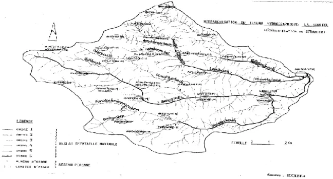
FIGURE 59 SOUFFEL HYDROGRAPHIC SUB-CATCHMENT 127

FIGURE 60 SOUFFEL ZONES 127

FIGURE 61 SOUFFEL HYDROGRAPHIC ZONES 128

FIGURE 62 CATCHMENT SECTION LAND USE COEFFICIENTS 130

FIGURE 63 CATCHMENT SECTION ALLOCATION KEY 131

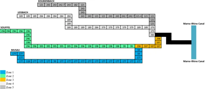
FIGURE 64 NITRATE DIFFUSE MASS FROM AGRICULTURAL SOURCES (mg/s) 132

FIGURE 65 CUMULATED NITRATE MASS FROM AGRICULTURAL SOURCES (mg/s) 132

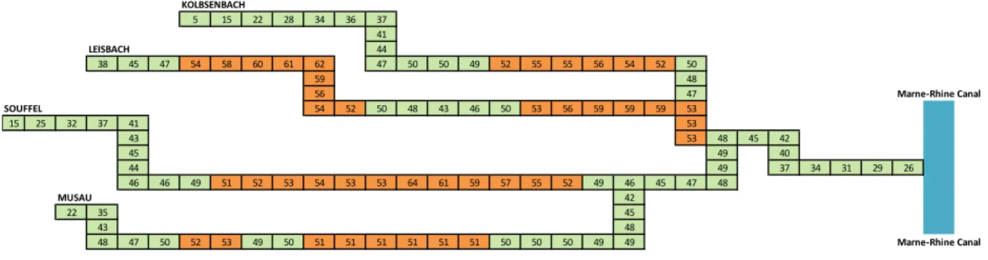
FIGURE 66 NITRATE CONCENTRATION FROM AGRICULTURAL SOURCES (mg/l) 133

FIGURE 67 NITRATE CONCENTRATION IN THE SOUFFEL CATCHMENT (mg/l) 134

FIGURE 68 DENSITY PLOT (LEFT) AND BOXPLOT (RIGHT) OF TOTAL CONCENTRATION 134

FIGURE 69 TOTAL NITRATE CONCENTRATION 136

FIGURE 70 TOTAL NITRATE CONCENTRATION DISTRIBUTION (AGRICULTURAL AND

ANTHROPOGENIC SOURCES) 136

FIGURE 71 CONSEQUENCE OF NITROGEN REDUCTION BY 28% FROM ALL ANTHROPOGENIC

POLLUTION SOURCES (SCENARIO 1) 137

FIGURE 72 CONSEQUENCE OF NITROGEN REDUCTION BY 37% FROM AGRICULTURAL SOURCES

(SCENARIO 2) 138

FIGURE 73 DATA DISTRIBUTION IN EACH MONITORING STATION 140

FIGURE 74 DETERMINATION OF THE MEDIAN DISTRIBUTION BY MONTE CARLO 143

FIGURE 75 MCS RESULTS 143

FIGURE 76 QQ PLOT MCS 144

FIGURE 77 MINIMAL NITRATE CONCENTRATION (- 4 mg/l) 145

FIGURE 78 MAXIMAL NITRATE CONCENTRATION (+ 4 mg/l) 145

FIGURE 79 RIVER FLOW WITH THREE WWTPs 147

FIGURE 80 URBAN NITRATE DISCHARGED MASS WITH THREE WWTPs (mg/s) 148

FIGURE 81 NITRATE CUMULATED MASS WITH THREE WWTPs (mg/s) 148

FIGURE 82 NITRATE CONCENTRATION FROM URBAN SOURCES WITH THREE WWTPs (mg/l) 149

FIGURE 83 NITRATE CONCENTRATION FROM AGRICULTURAL SOURCES WITH THREE

WWTPs(mg/l) 149

FIGURE 84 NITRATE CONCENTRATION IN THE CATCHMENT WITH THREE WWTPs (mg/l) 150

FIGURE 85 DENSITY PLOT (LEFT) AND BOXPLOT (RIGHT) OF TOTAL CONCENTRATION WITH

(16)

15

FIGURE 86 TOTAL NITRATE CONCENTRATION WITH THREE WWTPs 152

FIGURE 87 TOTAL NITRATE CONCENTRATION DISTRIBUTION (AGRICULTURAL AND

ANTHROPOGENIC SOURCES) WITH THREE WWTPs 153

FIGURE 88 CONSEQUENCE OF NITROGEN REDUCTION BY 25% FROM ALL ANTHROPOGENIC

POLLUTION SOURCES (THREE WWTPs) 153

FIGURE 89 CONSEQUENCE OF NITROGEN REDUCTION BY 25% FROM AGRICULTURAL SOURCES

(THREE WWTPs) 154

FIGURE 90 MINIMAL NITRATE CONCENTRATION (-4 mg/l) WITH THREE WWTPs 155

FIGURE 91 MAXIMAL NITRATE CONCENTRATION (+ 4 mg/l) THREE WWTPs 156

FIGURE 92 PRESENT VALUE IN EURO OF THE NITROGEN ABATEMENT COST FOR SCHOU ET AL.

(2006) 159

FIGURE 93 CORN YIELD VS NITROGEN APPLICATION 160

FIGURE 94 ABATEMENT COST FUNCTION 161

FIGURE 95 DAMAGE WITH UNIFORM VULNERABILITY FOR AN OVERALL DAMAGE OF 1 M €/YEAR

168

169

FIGURE 98 SOUFFEL POPULATION DISTRIBUTION 170

FIGURE 99 INHABITANTS LOCATED IN SPOTS LESS THAN 5 KM FROM EACH CATCHMENT

SECTION 171

FIGURE 100 DAMAGE WITH HETEROGENEOUS VULNERABILITY FOR AN OVERALL DAMAGE OF

1 M €/YEAR 172

2 M €/YEAR 173

3 M €/YEAR 173

FIGURE 103 OPTIMAL NITRATE CONCENTRATION (mg/l) FOR A UNIFORM DAMAGE OF 1 M €/YEAR

175

176

177

FIGURE 106 OPTIMAL NITRATE CONCENTRATION (mg/l) FOR A HETEROGENEOUS DAMAGE OF

1 M €/YEAR 178

2 M €/YEAR 178

3M €/YEAR 179

FIGURE 109 CURRENT POLLUTION (mg/l) AND CURRENT MONITORING STATIONS 183

FIGURE 110 NITRATE CONCENTRATION (mg/l) AFTER NITROGEN REDUCTION FOR THE CURRENT

MONITORING NETWORK 184

FIGURE 111 CURRENT POLLUTION (mg/l) AND PHYSICALLY OPTIMIZED MONITORING NETWOR 185 FIGURE 112 NITRATE CONCENTRATION (mg/l) AFTER NITROGEN REDUCTION FOR THE

PHYSICALLY OPTIMIZED MONITORING NETWORK 186

FIGURE 113 CURRENT POLLUTION (mg/l) AND ECONOMICALLY OPTIMIZED MONITORING

NETWORK FOR UNIFORM OVERALL DAMAGE OF 1 M €/YEAR 187

FIGURE 114 NITRATE CONCENTRATION (mg/l) AFTER NITROGEN REDUCTION FOR THE

ECONOMICALLY OPTIMIZED MONITORING NETWORK FOR OVERALL UNIFORM DAMAGE OF

(17)

16

NETWORK FOR HETEROGENEOUS OVERALL DAMAGE OF 1 M €/YEAR 189

ECONOMICAL MONITORING NETWORK FOR OVERALL HETEROGENEOUS DAMAGE OF

1 M €/YEAR 190

NETWORK FOR OVERALL UNIFORM AND HETEROGENEOUS DAMAGES OF 2 M €/YEAR AND

3 M €/YEAR 190

ECONOMICALLY OPTIMIZED MONITORING NETWORK FOR OF 2 M €/YEAR AND 3 M €/YEAR

OVERALL DAMAGE 191

FIGURE 119 EVOLUTION OF CONCENTRATIONS AS A FUNCTION OF OVERALL DAMAGE 193

FIGURE 120 LOCALISATION DES STATIONS DE SURVEILLANCE DANS UN RESEAU PHYSIQUEMENT

OPTIMISE 217

FIGURE 121 LOCALISATION DES STATIONS DE SURVEILLANCE DANS UN RESEAU ECONOMIQUEMENT

OPTIMISE (SCENARIO DE VULNERABILITE UNIFORME) 217

OPTIMISE (SCENARIO DE VULNERABILITE DECROISSANTE) 217

OPTIMISE (SCENARIO DE VULNERABILITE CROISSANTE) 217

FIGURE 124 EVOI POUR UNE VULNERABILITE UNIFORME 218

FIGURE 125 EVOI POUR UNE VULNERABILITE DECROISSANTE 218

FIGURE 126 EVOI POUR UNE VULNERABILITE CROISSANTE 219

FIGURE 127 VARIATION DE L’EVOI EN FONCTION DE L'INTENSITE SPATIALE ET TEMPORELLE DE LA

MESURE 220

FIGURE 128 DESIGN SPATIO-TEMPOREL OPTIMAL DANS LE SCENARIO UNIFORME (GAUCHE) ET LE

SCENARIO DECROISSANT (DROITE) 221

FIGURE 129 SCHEMA DU BASSIN VERSANT DE LA SOUFFEL 222

FIGURE 130 ZONES HYDROGRAPHIQUES SUR LA SOUFFEL 224

FIGURE 131 CONCENTRATION EN NITRATE SUR L’ENSEMBLE DE LA SOUFFEL (MG/L) 224

FIGURE 132 CONCENTRATION EN NITRATE SUR LA SOUFFEL AVEC TROIS STATIONS D'EPURATION

(mg/l) 225

FIGURE 133 COUT DE REDUCTION DE L’AZOTE PAR HECTARE ET PAR AN 226

FIGURE 134 ÉVOLUTION DES CONCENTRATIONS EN FONCTION DES DOMMAGES GLOBAUX 230

List of tables

TABLEAU 1 GRILLE DE 1971 41

TABLEAU 2 LOCALISATIONS ECONOMIQUEMENT OPTIMISEES DES STATIONS POUR LE SCENARIO 1 77 TABLEAU 3 DIFFERENCE ENTRE LES DEUX VEI POUR LE SCENARIO 1 78

TABLE 8 SOUFFEL CATCHMENT POPULATION 106

TABLE 9 MONITORING OBJECTIVES 110

TABLE 10 IDENTIFIED AVERAGE RIVER FLOW PER CATCHMENT SECTION 116

(18)

17

TABLE 12 LAND USE COEFFICIENTS DESCRIPTION 129

TABLE 13 SUM OF THE LAND USE COEFFICIENTS 130

TABLE 14 ZONE DIFFUSE COEFFICIENT 131

TABLE 15 DATA SUMMARY FOR THE NITRATE SOURCES AND THE TOTAL NITRATE

CONCENTRATION 135

TABLE 16 DATA SUMMARY FOR NITRATE REDUCTION FROM AGRICULTURAL AND URBAN

SOURCES 138

TABLE 17 DATA SUMMARY FOR NITRATE REDUCTION FROM AGRICULTURAL SOURCES 138

TABLE 18 DATA SUMMARY OF THE MEASURED NITRATE CONCENTRATION 139

TABLE 19 DATA SUMMARY OF THE MEASURED NITRATE CONCENTRATION 141

TABLE 20 NORMALITY TEST FOR EACH MONITORING STATION 142

TABLE 21 SHAPIRO-WILK TEST 144

TABLE 22 QUANTITY OF NITROGEN TREATED 147

TABLE 23 DATA SUMMARY FOR THE NITRATE SOURCES AND THE TOTAL NITRATE

CONCENTRATION WITH THREE WWTPs 151

TABLE 24 DATA SUMMARY FOR NITRATE REDUCTION FROM AGRICULTURAL AND URBAN

SOURCES (THREE WWTPs) 154

TABLE 25 DATA SUMMARY FOR NITRATE REDUCTION FROM AGRICULTURAL SOURCES

(SCENARIO “THREE WWTPs”) 155

TABLE 26 CONSTRUCTION OF THE ABATEMENT COST (BY YEAR) 161

TABLE 27 ESTIMATED DAMAGE FOR THE SOUFFEL CATCHMENT (€/YEAR) 165

TABLE 28 MARGINAL DAMAGE FOR DIFFERENT LEVELS OF OVERALL DAMAGE 167

TABLE 29 POPULATION PER SPOT 170

TABLE 30 CATCHMENT DAMAGE COEFFICIENT 172

TABLE 31 OPTIMAL NITROGEN REDUCTION FOR OVERALL UNIFORM DAMAGE OF 1 M €/YEAR 174 TABLE 32 OPTIMAL NITROGEN REDUCTION FOR OVERALL UNIFORM DAMAGE OF 2 M €/YEAR 175 TABLE 33 OPTIMAL NITROGEN REDUCTION FOR OVERALL UNIFORM DAMAGE OF 3 M €/YEAR 176 TABLE 34 OPTIMAL NITROGEN REDUCTION FOR OVERALL HETEROGENEOUS DAMAGE OF

1 M €/YEAR 177

TABLE 35 OPTIMAL NITROGEN REDUCTION FOR OVERALL HETEROGENEOUS DAMAGE OF

2 M €/YEAR 178

TABLE 36 OPTIMAL NITROGEN REDUCTION FOR OVERALL HETEROGENEOUS DAMAGE OF

3 M €/YEAR 179

TABLE 37 OPTIMAL UTILITY 179

TABLE 38 OPTIMAL NITROGEN REDUCTIONS 180

TABLE 39 NITROGEN REDUCTION FOR CURRENT MONITORING NETWORK 183

TABLE 40 NITROGEN REDUCTION FOR PHYSICALLY OPTIMIZED MONITORING NETWORK 185

TABLE 41 NITROGEN REDUCTION FOR ECONOMICALLY OPTIMIZED MONITORING NETWORK FOR

UNIFORM DAMAGE OF 1 M €/YEAR 187

HETEROGENEOUS DAMAGE OF 1 M €/YEAR 189

UNIFORM AND HETEROGENEOUS VULNERABILITY OF 2 M €/YEAR AND 3 M €/YEAR OVERALL

DAMAGE 191

TABLE 44 COST AND AVOIDED DAMAGES FOR THE DIFFERENT SCENARIOS 192

TABLE 45 ADVANTAGE OF ECONOMIC OPTIMIZATION 193

TABLEAU 46 REDUCTION OPTIMALE DE L’AZOTE 227

TABLEAU 47 UTILITÉS OPTIMALES 227

TABLEAU 48 EVOIs POUR LES DIFFERENTS RESEAUX ET SCENARIOS 229

(19)

18

List of abbreviations, acronyms, initials, and symbols

𝑎: Action

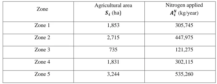
𝐴_𝒾𝑁: Total nitrogen quantity applied for zone 𝒾

𝐴_𝒾𝑗NO3−_: _{Nitrate mass for catchment section 𝑗 in the zone 𝒾}

𝐴̃_𝒾𝑗𝑁𝑂3−

: Nitrate cumulated mass for catchment section j in the zone 𝒾 ADES: Accès aux Données sur les Eaux Souterraines

AFB: Agence Française pour la Biodiversité

APRONA: Association pour la Protection de la Nappe Phréatique de la Plaine d’Alsace

ARS: Agence Régionale de Santé

𝐵_𝑒: Benefits (avoided damages) with economical optimization 𝐵_𝑝: Benefits (avoided damages) with physical optimization

BRGM: Bureau de Recherche Géologiques et Minières

BNDE: Banque Nationale des Données sur l’Eau

BV: Bequest value

𝐶: Cost of action

𝐶𝑒: Abatement cost with economical optimization

𝐶𝑝: Abatement cost with physical optimization

𝒞

𝐴_𝒾𝑗𝑁𝑂3

−_: Nitrate concentration from agricultural sources for catchment section 𝑗 in the zone

𝒾 𝒞₂₅

𝑗

𝑁𝑂3−_: _{Number of concentration units above 25 mg/l from catchment section 𝑗}

CI: Confidence Interval

𝐷: Environmental Damage

DBO5: Demande Biochimique en Oxygène à 5 jours

DCE: Directive Cadre sur l’Eau

(20)

19

DIREN: Directions Régionales de l’Environnement

DM: Decision Maker

DREAL: Direction Régionale de l’Aménagement et de Logement

EDF: Electricité de France

ERU: Eaux Résiduaires Urbaines

EV: Existence Value

EVOI: Economic Value of Information

GWR: Great Western Ring of Strasbourg project

𝐼: Random variable, which corresponds to the additional information provided by the network

ℐ: Number of agricultural zones

𝑖: Message that can be delivered by the network

𝒾: Agricultural zone

Ifremer: Institut Français de Recherche pour l’Exploitation de la MER INP: Inventaire National du degré de Pollution

𝐽_𝒾: Number of catchment sections in the zone 𝒾

𝐾: Potential states of nature and actions

ϰ: Catchment damage coefficient

𝑙: Location of the monitoring station in the river LEMA: Loi sur l’Eau et les Milieux Aquatiques

m: Multiplying coefficient

MCS: Monte Carlo Simulation

𝑚𝑢: Monetary Unit

𝑛: Number of monitoring stations

N: Nitrogen

NO₃−_: _{Nitrate concentration}

(21)

20

ONEMA: Office National de l’Eau et des Milieux Aquatiques

OV: Option Value

𝑃: Probability of emission of accidental pollution

p.e.: Population equivalent

𝑃(𝑖𝑠): Probability that the network sends the message 𝑖 indicating the state 𝑠

𝓅_𝑗: Population located in spots less than 5 km from catchment section 𝑗 𝑃(𝑠/𝑖_𝑠) ∶ Probability of being in the state 𝑠 when the network indicates 𝑖_𝑠

PAE: Programmes d’Action Environnementale

PAR: Programme d’Action pour le Rhin

𝑄_𝒾: Nitrogen quantity applied in the zone 𝒾

Ʀ𝒾𝑗: River flow for the catchment section 𝑗 in the zone 𝒾

RCB: Réseau Complémentaires de Bassin

RCO: Réseau du Contrôle Opérationnel

RCS: Réseau du Contrôle de Surveillance

RESALTT: Réseau de Surveillance des Tendances à Long Terme

RID: Réseau d’Intérêt Départemental

RNB: Réseau National de Bassin

RNDE: Réseau National des Données sur l’Eau

RNES: Réseau National de connaissances des Eaux Souterraines

𝑠: State of nature

𝑆𝐷: Average of the standard deviation

𝑆_𝒾: Agricultural area of the zone 𝒾

SAGE: Schéma d’Aménagement et de Gestion d’Eau

SANDRE: Service d’Administration Nationale des Données et Référentiels sur l’Eau

SDAGE: Schéma Directeur d’Aménagement et de Gestion d’Eau

SDEA: Syndicat des Eaux et de l’Assainissement Alsace-Moselle

(22)

21 SEEE: Système d’Evaluation de l’Etat des Eaux SEQ: Système d’Evaluation de la Qualité

SIE: Système d’Information sur l’Eau

SMET: Screening Methods and Emerging Tools

𝑇: The time or distance of detection of accidental pollution 𝑈𝑎/𝑠: Utility of the action 𝑎 when the state of nature is 𝑠

𝑢𝑚: Unité Monétaire quelconque

UV: Use Value

𝑣°(𝑙): Uniform vulnerability 𝑣−(𝑙): Decreasing vulnerability 𝑣+(𝑙): Increasing vulnerability

VEI: Valeur Economique de l’Information

WFD: Water Framework Directive

WQMN: Water Quality Monitoring Network

WWTP: Waste Water Treatment Plant

𝑥̿: Average of the mean

ZPS: Zone de Protection Spéciale

ZSC: Zone Spéciales de Conservation

𝛼: Probability of no detection of accidental pollution

𝛽: Fixed budget of the network manager

𝛿: Marginal damage

Ө: Monitoring cost

𝜆: Slope of the monitoring cost function

𝜋: Net benefit of monitoring

𝜄𝒾𝑗: Land use coefficient for the catchment section 𝑗 in the zone 𝒾

𝜌: Auto-purification coefficient

(23)

22

𝜎̂: Standard deviation of the normal distribution

(24)

23

CHAPTER I: General introduction

Water is a natural resource that is essential for human existence and for many other species that use this resource as a drinking source and natural habitat. It is important for human development as it allows human activities like agriculture, industrial use, fishing, etc. Water resources cover almost 70% of our planet. However, 2.6% of water is freshwater that is intended for human consumption, from which 1.6% is under the form of glaciers (Budzinski et al., 2013). Therefore, only 1% of fresh water is available in liquid form. Thus, it is a scarce resource that we need to protect.

“The 2018 edition of the United Nations World Water Development Report stated that nearly 6

billion peoples will suffer from clean water scarcity by 2050. This is the result of increasing demand for water, reduction of water resources, and increasing pollution of water, driven by dramatic population and economic growth” (Boretti and Rosa, 2019).

The preservation of water quality then became a priority in developed and developing countries around the world. For that particular reason, goal 6 of the United Nations Sustainable Development Goals is: “Clean Water and Sanitation”1_.

Water pollution issue

Over the years, water usage has been gradually diversified and intensified in different forms (domestic, agricultural, and industrial). This diversification led to an increase in water pollution (Budzinski et al, 2013).

Water pollution is not a recent problem, although for a long time it has remained a local and small-scale problem. According to Gioda (1999), heavy metals, widely used, are among the most important chemical pollutants as early as Antiquity. For example, the water conducts in ancient Rome were constructed mainly of lead, which caused the discharge of lead materials into the streams. Also, mercury has been used in silver metallurgy. Mercury was commonly used in

(25)

24

medicines to cure diseases like Syphilis and Leprosy, and lead was used to glaze pottery2_.

Finally, urban waste was tossed in streets and then discharged into water streams when the streets were cleaned, generating pollution by pathogenic bacteria and fermentable substances. The industrial revolution of the 1800s increased the energy needs for countries using first coal and then petrol to meet the energy needs. Fossil fuels became the source of countless air, water, and soil pollution. Factories found the water a convenient mean of waste disposal. Water resources were also contaminated by rain runoff from oil-slick roads, construction, mining, dump sites, and livestock wastes from farm operations3. About agriculture, the first chemical fertilizers appeared in 1838, and the first pesticides in 1885 with the Bordeaux mixture of copper and sulfate (Gioda, 1999), although it was not until the middle of the 20th century that these agricultural techniques became widespread.

Finally, the period of post-World War II reconstruction was marked by unprecedented industrial and agricultural development. Water pollution has become a global problem. Nowadays, water pollution problems remain a concern. Despite the actions implemented to reduce certain pollutants, some of them persist and others are appearing such as diffuse pollution or micro-pollutants. Water pollution is a global challenge that has increased in both developed and developing countries undermining economic growth as well as the physical and environmental health of billions of people (FAO and IWMI, 2017). Globally, 80% of untreated municipal wastewater is discharged into aquatic environments, and the industry is responsible for dumping millions of tons of heavy metals, solvents, toxic sludge, and other wastes into the water each year (FAO and IWMI, 2017). According to UN WWAP (2003), every day 2 million tons of sewage, industrial and agricultural waste is discharged into the world's water. Agricultural is the dominant source of water pollution around the world, it contributes to 70% of water abstractions worldwide and discharges large quantities of agrochemicals, organic matter, drug residues, sediments, and saline drainage.

In the European Union, only 40% of rivers, lakes, estuaries, and coastal waters reach the ecologically acceptable standard and 38% are in good chemical status in 20184. The main significant pressures on surface waters are hydro-morphological pressures, diffuse sources,

2_{https://www.smithsonianmag.com/smart-news/lead-poisoning-made-medieval-townspeople-sickly-180957021/}

3_{https://www.history.com/topics/natural-disasters-and-environment/water-and-air-pollution}

(26)

25

particularly from agriculture, and atmospheric deposition, particularly of mercury, followed by point sources and water abstraction5_{. Specifically, 38% of surface waters are significantly under}

pressure from agricultural pollution (FAO and IWMI, 2017).

Water quality regulation

In France, water regulation goes back to Imperial times. The Civil code determined the ownership and use of water in various watercourses. Article 714 specifies, among other things, a property that has no owner is the property of the public. Thus, all individuals had the right to use such public property such as air or water. However, the Civil code did not mention any quality obligations.

The first regulation concerning water pollution goes back to the Imperial decree of 15 October 1810. The Imperial decree is considered one of the acts inaugurating the sanitary control of industrial pollution. Originally, it was aimed primarily at sodium factories and factories emitting acid and chlorine emissions. Article 1 of the Imperial decree precise that, as of the publication of the decree, the factories, and workshops that spread an unhealthy or uncomfortable smell cannot be formed without permission from the administrative authority6. The decree divides the establishments into three categories: the first includes those who have to be moved away from private houses; the second is factories and workshops whose distance from homes is not strictly necessary but whose operations are allowed after it is certain that they are carried out in such a way as not to disturb or cause damage to the owners in the neighborhood, and the third is the establishment which may remain without inconvenience near houses but must remain under police surveillance.

The main concern regarding the water quality was raised in the post-World War II period. This can be explained by the high water quality deterioration caused by reconstruction and industrial activities (Bouleau, 2014). This led to the drafting of the first water law (law n° 64-1245 of 13 December 1964 concerning the regime and distribution of waters and the fight against their pollution) in 1964. The water act organized water management in the French territories. It is

5

https://www.eea.europa.eu/themes/water/european-waters/water-quality-and-water-assessment/water-assessments/eea-2018-water-assessment

(27)

26

considered the foundation of what has become the French school of water management. It consisted of decentralized water management by the catchment area. It divided the French territories into six catchment areas: “Rhin-Meuse”, “Rhône-Méditerranée”, “Adour-Garonne”, “Loire-Bretagne”, “Seine-Normandie”, and “Artois-Picardie”. The law created Basin Committees and the application of the polluter pays principle through the Basin Financial Agencies. One of the main responsibilities of the agencies is to give subsidies and loans to public and private persons for the execution of works of common interest. Also, the agencies must establish and collect charges from public or private persons under the extent that such public or private persons require or make it necessary or useful for the intervention of the agency. It was the first law in France that intended to control water pollution.

In 1976 a new law concerning the classified installation for the protection of the environment (law n°76-663 of 19 July 1976) was adopted, and it became the legal basis for the industrial environment in France. The law of 1976 is an extension of the 1810 Imperial decree. The regulation of classified installation is a special police measure enabling the government to monitor and control installations and activities with dangers or inconveniences for the environment.

Since the 1970s the French public policy of water is part of the European framework. Several European Directives were introduced concerning the water quality and more specifically to the reduction of water pollution from different sources. From 1970 to 1990, two waves of European Directives concerning water quality were adopted. The first wave took place from 1975 to 1980. This wave gave rise to several Directives concerning environmental quality standards or the establishment of emission limit values for specific water uses Directive 75/440/EEC on surface water (1975); Directive 76/464/EEC on dangerous substances (1976); Directive 78/659/EEC on fish waters (1978); Directive 79/923/EEC on shellfish waters (1979); Directive 80/86/EEC on groundwater (1980). The second wave of Directives took place in the 1990s, more specifically in 1991 with two Directives establishing obligations of means to limit specific discharges: Directive 91/676/EEC also called Nitrate Directive (1991); and Directive 91/271/EEC on urban wastewater treatment (1991). This led to the adoption of the second water law in France in 1992. The second water act recognizes water as a national heritage and gives importance to preserving

(28)

27

this heritage for future generations. Hence, the 1992 water act introduces sustainable development terms to water resources.

To have a more harmonized water policy in the European Union, the European Commission adopted on 23 October 2000 the Water Framework Directive (WFD) (Directive 2000/60/EC) establishing a community policy in the field of water policy. Unlike the other European Directives, the WFD sets result in objectives to be achieved within a specific deadline (2015, 2021, 2027 cycles). It takes up the French principles of decentralized river basin management and imposes a common method to all member states. Moreover, in each country aquatic environments are divided into geographical units called water bodies. According to article 5 of the Directive, each member state shall ensure, for each water body within its territory, analysis of its characteristics, a review of the impact of human activity on the status of surface waters and groundwater, and finally an economic analysis. The economic analysis of water bodies involves carrying out a cost-effectiveness analysis to select the measures that should be put in place to achieve good status, then a cost-benefit analysis, which compares the cost of achieving goods status with the environmental benefit (or avoided damage). If the cost is higher, an exemption may be obtained for economic reasons. The good status may, therefore, be achieved later or a less stringent standard can be defined. For each river basin, each member state shall ensure a program of measures taking into account the results of the analysis done. The Directive was transposed into French law by the law of 30 December 2006, also known as the LEMA (Loi sur

l’Eau et les Milieux Aquatiques, n° 2006-1772).

Water quality monitoring

All the national laws and European Directives intended to establish a water quality management plan to stop water degradation. However, to act on water pollution requires knowledge and a full understanding of the water quality. This led the public authorities to develop programs over the years to retrieve information regarding water quality. Retrieval of such information requires collecting data. The objective of collecting data is to produce information for the efficient management of the water environment. Thus, Water Quality Monitoring Networks were developed in almost all countries to monitor water quality (Harmancioglu et al., 1999).

(29)

28

Water Quality Monitoring Network (WQMN) can be defined as all sampling activities to collect and process data on water quality to obtain information about the physical, biological, and chemical properties of water. Their role is to provide sufficient information to enable Decision Makers (DM) to make informed decisions about the health risks associated with people’s exposure to water resources (Telci et al., 2009).

According to Harmancioglu et al. (1999), the first WQMN appeared in Netherland in 1950. It consisted of monitoring water quality in four sites by observing some variables. The monitoring networks were then expanded in other developed countries and developing countries after that. In Chapter 2 of this dissertation, we present an overview of the history of the WQMN in France.

Water quality monitoring networks design optimization

The DM relies on the information communicated by the monitoring networks regarding the water quality to make decisions, which can be modified. Therefore, the effectiveness of the decision depends on the relevance of the information given by this network. Thus, optimizing the WQMN design has been the subject of numerous research papers. What is called network design here, is the choice of the number and location of the monitoring stations (spatial issue), as well as the frequency of this measurement (temporal issue). In this first type of literature on the WQMN, the studies aimed at optimizing the monitoring network by taking only physical or hydrological considerations into account.

Papers that focused on the spatial aspects of optimization aim to find the location of a fixed number of stations that minimizes inaccuracies in pollution information. Several authors have addressed this issue. Alvarez-Vázquez et al. (2006) use a theoretical approach to determine the optimal location of the sampling stations in a river with wastewater discharge. They determined the location of the monitoring stations that decreased the average deviation from the average water pollution. Telci et al. (2009), for their part, focused on determining the location of the stations in the Altamaha river basin (Georgia – USA) that minimized the detection time for accidental pollution. For Destandau and Point (2000), the location of the stations aimed at the identification of blackspots in a river of the “Adour-Garonne” catchment area (France). Respecting a quality standard in these points ensures that it is respected everywhere. Finally,

(30)

29

Park et al (2006) use a genetic algorithm to resolve a multi-objective network including representativeness of the river system, compliance with water quality standards, supervision of water use, surveillance of pollution sources, and examination of water quality changes. The method was applied to the Nakdong river (Korea).

The articles that focused on the temporal aspects of optimization aim to minimize frequency while retaining the desired information. It’s about eliminating redundant information. For example, in Liu et al. (2014) the objective of the network to know the average annual pollution within a predefined confidence interval; in Naddeo et al. (2013) to determine the pollution trend: upward, downward or no trend; and in Kim et al. (2007) to determine the seasonal variation of water quality. Finally, Zhou (1996) implemented a multi-objective model with these three objectives: trend detection, determination of periodic fluctuation, and estimation of mean values of the stationary component.

More recently, Pourshahabi et al. (2018) found the optimal spatio-temporal design of a WQMN in the Karkheh reservoir (Iran). They presented a multi-criteria methodology to determine the optimal location and number of monitoring stations, but also the optimal sampling frequency. Optimizing the design of a monitoring network implies that the information provided can be increased. This raises the question of the information quantification.

Information quantification

Information can be seen as a numerical quantity that measures the uncertainty in the outcome of an experiment to be performed. This was developed in the work of Shannon (1948) on the information theory.

The information theory studies the transmission, processing, extraction, and utilization of information which is considered as a set of possible messages. The objective is to quantify the average information content of this set of messages. It is a probability theory that considers information as a set of possible messages and their probability of occurrence. Information quantification depends solely on the probability of the message. If a message is very likely to happen, it contains little information. Indeed, if an information source always sends the same

(31)

30

message, the uncertainty about the future message will be minimal. The amount of information is therefore also minimal. Conversely, if a message is unlikely to happen, it contains much information. In this case, the information has a greater benefit to the recipient. Thus, the amount of information contained in a message is inversely proportional to the probability of its appearance7.

On this principle, Shannon calculates the amount of information contained in a set of messages using the entropy mathematical formula. Shannon's entropy measurement represents the surprise effect caused by message transmission. Entropy will be maximum for equiprobable messages. One of the limitations of Shannon's information theory is that it does not take into account the usefulness of the messages to the receiver. What value does this information have for the receiver?

What is Value?

The concept of value is used in a great variety of contexts and “value” has many meanings. It can be used to signify standards, beliefs, principles, moral obligations, and social norms, but also, desires, wants, needs, or interests (Pauls, 1990). For Kenyon and Sen (2015), value is defined as “desirable, transituational goal, varying in importance that serves as guiding principles in people's lives”

Value is an interdisciplinary concept used in many scientific disciplines such as philosophy, sociology, psychology, and economic sciences (Wiechoczek, 2016).

Each discipline has its definition of value. In this dissertation, we focus exclusively on the term value in economics.

Economic value

Value is a concept at the very foundation of the economy. Economists see value as something that helps define wealth (Delecroix, 2005).

(32)

31

In economics, the term value is based on what we call the theories of value that seek to explain the functioning of the economy, the price formation of goods and services in the markets (Malmaeus, 2016). We can distinguish value theories into two main categories: objective (classical value theory) and subjective (neoclassical value theory) (King and McLure, 2014). The classical value theory, or the labor theory of value, dates back from the mid-to-late 18th century and was mainly based on the work of Adam Smith, David Ricardo, and Karl Marx. The labor theory of value was first introduced by Adam Smith in his book “The Wealth of Nations”. According to Smith:

“The word value, it is to be observed, has two different meanings, and sometimes expresses the utility of some particular object, and sometimes the power of purchasing other goods which the

possession of that object conveys. The one may be called value in use; the other value in exchange” (Smith, 1776).

According to Adam Smith, the term value can be used in two senses, the value in use and value in exchange8. Value in use is the want satisfying power of a commodity. It is the satisfaction which an individual obtains from the use of a commodity. On the other hand, the value in exchange is the amount of goods and services which an individual may obtain in the market in exchange for a particular thing. It is the price of a particular good that can be sold and bought in the market. From another point of view, David Ricardo provides another treatment of the value theory. Ricardo’s value theory holds that the value of a good is proportional to how much labor was required to produce it, including the labor required to produce the raw materials and machinery used in the process. Hence, he includes human labor time in the product. However, Ricardo did not distinguish between the different modes of production. For that, Marx believed that we need to distinguish between capitalism and the classless “simple” or “petty commodity production”. In simple commodity production, goods were sold at prices equal to their labor values but in capitalism, matters were considerably more complicated (King and McLure, 2014). The neoclassical value theory started to develop after the introduction of the concept of marginal utility in the 1870s (late 19th century) by William Stanley Jevons, Carl Menger, and Léon Walras (Malmaeus, 2016). In the neoclassical value theory, the classical principle for the value

(33)

32

determined by the production costs was replaced by the laws of demand and supply that were introduced by Alfred Marshall. The market equilibrium was set out at the intersection of the two curves of supply and demand. In this theory, we have started to see a relation between the market prices and consumers’ utility that was not present in the classical value theory. The combination of utilities and costs for the determination of prices is referred to as the neoclassical theory of value and is accepted by most economists and widely applied in general equilibrium models. According to this approach, the values are formed by interactions between agents in the market. According to Malmaeus (2016), classical and neoclassical value theories are the most interesting theories for explaining the real value of societal production. However, not all goods and services are exchanged in markets and have market value. These goods are often public goods provided by the government or environmental resources that everyone has the right to access (Pauls, 1990). What is the value attributed to this type of good or resource?

Environmental economics has developed many methods for estimating the value of environmental non-market goods and services: contingent valuation, travel cost, hedonic pricing, etc. (Abdullah et al., 2011). These methods attempt to estimate two types of values: Use Value (UV) and Non-Use Value (NUV). The UV is generated when a person uses an environmental service actively, typically by consuming it directly or combining it with other goods and services and the person’s own time to produce an activity that generates utility. On the other hand, the NUV is the idea that people might enjoy the satisfaction of just knowing that a particular habitat is being maintained in good condition (National Research Council, 1999). This value is not associated with the use of the resource or the tangible benefits deriving from its use. It can be subdivided into three sub-groups: the existence values (EVs); the bequest values (BVs) and the option value (OV) (Abdullah et al., 2011).

Following this review of the literature on the value in economics, and in particular the valuation of environmental goods, we will focus on the Economic Value of Information.

(34)

33

Economic Value of Information

Stigler (1961) is considered a pioneer in the information economy by showing that price differences can be explained by the presence of costs associated with finding and disseminating information. Several economic studies have tried to attribute value to information.

For example, Corbel (2013) applied Porter's Value Chain analysis to information. Porter's value chain is based on the different activities of a firm (procurement, human resources management, logistics, production, etc.). The way value chain activities are articulated determines costs and affects profits, so this tool can help the firm to analyze the sources of value creation. In his study on the concept of the value chain in knowledge economics, Corbel applies Porter’s value chain concept to the information system, to identify the role of information in increasing value.

Incentive theory also offers a way of estimating the value of information under asymmetric information (Laffont and Tirole, 1993). In a Principal-Agent model, when the Principal has only limited information on the characteristics of the Agent (adverse selection) and/or on his behavior (moral hazard), he could propose a menu of contracts to reveal this information. Better informed than the Principal about his characteristics and intentions, the Agent will choose the contract whose method of remuneration best suits the risks he wishes to take and the efficiency efforts he envisages. To be revealing, these contracts must, however, contain information rent, which can thus be assimilated to the value of the information held by the Agent.

However, for our study, these models are not very appropriate for the economic value of information coming from a WQMN. We prefer to build on Shannon’s information theory by adding decision theory. Decision theory is the study of the solution to a decision problem including the analysis of the option to seek the services of an information source (Lawrence, 1999). Thus, the Economic Value Of Information (EVOI) is defined as the increase in the expected value that arises from making the best choice with the benefit of a piece of information compared to the best choice without the benefit of this information (Keisler et al., 2013). This can also be equated to the amount that a DM would be willing to pay for information before making a decision.

The method for estimating EVOI that we will choose and call the Bayesian method is described at length in Hirshleifer and Riley (1979).

(35)

34

We assume that a DM has to choose between different “actions”. The utility generated by each action will depend on the “state of nature”. However, while making his decision, the DM has only probabilistic information about the state of nature, i.e., a priori probabilities associated with each state of nature that correspond to his initial beliefs. When the DM receives additional information (such as the information provided by a WQMN), he will correct his beliefs, i.e. transform the a priori probabilities associated with the states of nature into a posteriori probabilities according to Bayes' theorem. He will thus increase the probability of implementing actions more adapted to the state of nature, in other words, actions that will generate more utility. EVOI can be calculated as the difference between the utility generated by "informed" actions and the utility generated by actions that would have been taken without the additional information. This method has been used by several authors in different scientific fields like health (Koerkamp et al., 2010; Claxton et al., 2001), petroleum studies (Bickel, 2008; Santos et al., 2017), and fisheries management (Prellezo, 2017; Mäntyniemi et al., 2009).

Economic Value of Information of Water Quality Monitoring Networks

Recently, this method is used in the water management field. The literature aimed at calculating the EVOI with the Bayesian method of a predefined monitoring network. For example, Bouma et al. (2009) estimate the EVOI of satellite observation to manage water quality in the North Sea. This information is intended to better guide policies to reduce eutrophication. Bouma et al. (2011) assess the EVOI of satellite observation to improve Great Barrier Reef protection. This information is intended to choose between a spatialized or uniform policy to protect the reef. Destandau and Diop (2016) have a more theoretical approach. They identified the parameters that have an impact on the EVOI: prior probabilities on states of nature, costs linked to a bad decision, and the accuracy of additional information. They constructed a theoretical model to study the impact of these parameters on the EVOI. Khader et al. (2013) estimate the EVOI of the groundwater quality monitoring network. They use the decision tree model to choose between two alternatives: ignore health risk, and switch to alternative drinking Bouzit et al. (2013) assess the EVOI of water screening methods and emerging tools (SMETs9). The study combines three empirical applications. The first study consists of valuing information 9_{It is a term used for new techniques to measure water pollution more effectively.}

(36)

35

provided by an isotope monitoring campaign enabling the origin of nitrate pollution in groundwater to be identified. In the second study, the information assessed was derived from passive samplers and multi-parameter probe technology to collect accurate information on sources of pesticide pollution (urban or rural). The third case measures the EVOI of an automated alarm station that integrates SMET to prevent any toxic pollution.

The Ph.D. dissertation

As we have seen in this Introductory Chapter, we are interested intwo types of literature in the field of Water Quality Monitoring Networks. The first type shows that authors seek to physically optimize the network by looking for location and/or frequency of measurement that minimizes imprecision in quality estimation with a given number of stations or minimizing the frequency while retaining the desired information. The second type, authors estimate the Economic Value of Information of a predefined network with the Bayesian method.

In this Ph.D. dissertation, we combine, for the first time, both types of literature by using the EVOI to optimize a WQMN. Indeed, by focusing in particular on the question of the location of the monitoring stations, we optimize the design of the networks by maximizing the EVOI. We will talk about economic optimization.

This dissertation is organized as follows.

Chapter II presents an overview of the history of the Water Quality Monitoring Networks in France. We retrace the history of the networks for the national level and also for the local level, namely in the Rhine-Meuse watershed. For each monitoring network, we present the objective and design choices. This Chapter allows us to identify the network objectives for which our method can be applied. We choose two of them, which will be the subject of the next two chapters. This chapter was the subject of a paper published in the journal TSM (Zaiter and Destandau, 2020).

Chapter III presents our method of economic optimization in a theoretical model where the network is designed to detect accidental pollution. After an introductory Section, we show in Section 2 that the advantage of our method over traditional physical optimization will depend on