HAL Id: hal-01770431
https://hal.archives-ouvertes.fr/hal-01770431
Submitted on 19 Apr 2018HAL is a multi-disciplinary open access archive for the deposit and dissemination of sci-entific research documents, whether they are pub-lished or not. The documents may come from teaching and research institutions in France or abroad, or from public or private research centers.
L’archive ouverte pluridisciplinaire HAL, est destinée au dépôt et à la diffusion de documents scientifiques de niveau recherche, publiés ou non, émanant des établissements d’enseignement et de recherche français ou étrangers, des laboratoires publics ou privés.
Hybrid fuzzy-probabilistic approach to supply chain
resilience assessment
Dmitry Ivanov, Alexander Pavlov, Alexandre Dolgui, Boris Sokolov
To cite this version:
Dmitry Ivanov, Alexander Pavlov, Alexandre Dolgui, Boris Sokolov. Hybrid fuzzy-probabilistic ap-proach to supply chain resilience assessment. IEEE Transactions on Engineering Management, Insti-tute of Electrical and Electronics Engineers, 2018, 65 (2), pp.303 - 315. �10.1109/TEM.2017.2773574�. �hal-01770431�
Hybrid fuzzy-probabilistic approach to supply chain resilience assessment
Dmitry Ivanov1*, Alexander Pavlov2,4 , Alexandre Dolgui3, Boris Sokolov4 IEEE Transactions on Engineering Management
This is an old version of paper before the peer review
1
Berlin School of Economics and Law Prtofessor for Supply Chain Management 10825 Berlin, Germany
2
Mozhaisky Military Space Academy, 197198 St. Petersburg, Russia
3
Ecole des Mines de Nantes
IRCCYN, UMR CNRS 6597 La Chantrerie
4, rue Alfred Kastler - B.P. 20722, F-44307 NANTES Cedex 3, France E-mail: alexandre.dolgui@mines-nantes.fr
4
SPIIRAS, Saint Petersburg Institute of Automation and Informatics, Russian Academy of Sciences, 199178 St Petersburg, Russia
* Corresponding author Prof. Dr. habil Dmitry Ivanov
Professor for Supply Chain Management Berlin School of Economics and Law 10825 Berlin
Germany
E-Mail: divanov@hwr-berlin.de
Tel.: +49 (0)30 308771155
Abstract. In this paper, we extend the existing models of supply chain resilience assessment by incorporating the ripple effect and structure reconfiguration. The research is based on a hybrid fuzzy-probabilistic approach. We apply the genome method with the objective to include the structural properties of the supply chain design into resilience assessment. We develop a supply chain design resilience index, demonstrate its computation and application. The results suggest a method to compare different supply chain designs regarding the resilience with both disruption propagation and recovery consideration. It also allows identifying groups of critical suppliers whose failure interrupt the supply chain operation.
Keywords: supply chain engineering, risk management, resilience, structure dynamics, ripple
Introduction
The supply chain engineering under uncertainties is a major issue in production systems and lo-gistics (Dolgui and Proth, 2010). One of most challenging problems deals with an increase of supply chain resilience, especially facing ripple effect.
The ripple effect, also known as domino effect or snowball effect (Wierczek 2014) describes the disruption propagation in the supply chain (SC), the impact of a disruption on SC performance and the disruption-based scope of changes in the SC design (SCD) structures (Liberatore et al. 2012, Ivanov et al. 2014a,b, Sokolov et al. 2016). Managing the ripple effect is closely related to designing resilient SCs.
SC resilience became one of the key investigation categories over the last decade (Gunasekaran et al. (2015). SC resilience is understood in literature as an ability to maintain, execute and re-cover (adapt) the planned process states along with achievement of the planned (or adapted, but yet still acceptable) performance (Sheffi and Rice 2005, Ivanov and Sokolov 2013, Kamalahmadi and Mellat-Parast 2016a,b). Recent studies underline the crucial role of resilience assessment taking into account disruption risks (e.g., Ivanov et al. 2013, Munoz and Dunbar 2015, Das and Lashkari 2015, Ivanov et al. 2016).
The existing studies have mostly focused on the impact of disruptions on SC resilience using deterministic approaches and the reliability theory without considering structure reconfiguration (Wagner and Neshat 2010, Soni et al. 2014, Kim et al. 2015). Recently, the necessity of inclu-sion the reconfiguration into SC resilience analysis was manifested by Simchi-Levi et al. (2014), Xu et al. (2014), Snyder et al. (2016). However, to the best of our knowledge there is no pub-lished graph-theoretical research on SCD resilience analysis with both disruptions and recovery considerations. In addition, the existing studies (e.g., Kim et al. 2015) consider monotonous SC structures (i.e., the failures of structure elements lead to the reliability decrease and recovery of structure elements lead to SC reliability increase). In reality, SC structures can be non-monotonous, i.e., the factors such as competitor behavior can also influence the SC resilience (e.g., a failure of one competitor can lead to reliability increase).
In this study, the following problem is considered. The object of investigation is a multi-stage SC different elements of which can be disrupted. The problem is to identify the impact of disrup-tions at different SC locadisrup-tions on SC resilience and to identify the critical SC nodes and arcs the disruptions of which result in SC resilience loss.
The goal of this study is to develop a method for quantitative analysis of SCD resilience with disruption propagation and recovery considerations for both monotonous and non-monotonous
structures. We are also interested in developing an SCD resilience index that can be used by SC managers to compare different SCDs regarding the resilience.
The remainder of this paper is organized as follows. Section 2 provides a state-of-the-art over-view. In Section 3, the research methodology is presented. Section 4 describes the fuzzy-probabilistic approach and the underlying concept of graph genome. In Section 5, the modeling procedure for the SC structure dynamics with reconfiguration is described. In Section 6, the SCD resilience index is described. Section 7 is devoted to the experimental part. In Section 8, manage-rial insights are presented. The paper concludes by summarizing the most important insights from the research and delineating future research avenues.
2. Literature review
The ability to maintain and recover (adapt) the planned execution along with achievement of the planned (or adapted, but yet still acceptable) performance is related by most authors to SC
resili-ence (Bakshi and Kleindorfer 2009, Ivanov and Sokolov 2013, Xu et al. 2014, Ambulkar et al.
2015). It can be observed in the existing studies that two groups of problem statements for SC resilience analysis are generally considered (see Fig. 1):
Resilience consideration without recovery measures and Resilience consideration with recovery measures.
Fig.1. Disruption consideration without and with recovery measures
We limit the literature analysis to graph-theoretical approaches taking into account the focus of this research. Stochastic Petri nets have been applied to analyse disruption propagation through the SC and to evaluate the performance impact of the disruptions (Wu et al. 2007). Wang and Ip (2009) and Soni et al. (2014) develop resilience metrics with the use of graph theory. Wagner and Neshat (2010) propose a method of quantifying risk using the permanent of an adjacency matrix based on graph theory. Nair and Vidal (2010) analyse the correlation between disruption
and structural features of network. Hsu and Li (2011) develop a method to evaluate reliability of the SC performance under the demand fluctuations.
Schoenlein et al. (2013) define robustness as the ability of a multiclass queuing network to re-main stable, if the expected values of the inter-arrival and service time distributions are subject to uncertain shifts. Based on the fluid network analysis they present a measure to quantify the robustness called the stability radius. Ivanov and Sokolov (2013) describe SC stability, robust-ness, and resilience as an integrated control problems within the framework of automatic control theory. Zobel and Khansa (2014) quantify resilience of supply chain for multiple disruptive events. Xu et al. (2014) develop a quantitative model for analysis of predicted SC resilience based on structural evolution against random supply disruptions. The study by Lin et al. (2014) concentrates on the reliability assessment for a multi-state SC with multiple suppliers as the probability to satisfy the market demand within the budget and production capacity limitations. They develop an algorithm in terms of minimal paths to evaluate the network reliability along with a numerical example regarding auto glass. Garvey et al. (2015) build upon minimal paths analysis and suggest using Bayesian network to analyse risk propagation in the SC. This is an interesting research avenue. Bayesian networks have also been applied to domino effect analysis in chemical industry infrastructures (Khakzad 2015).
Another important research stream has been the understanding that different kinds of SCD struc-tures with similar number of nodes and arcs may significantly differ regarding resilience. Bode and Wagner (2015) analyse empirically structural drivers of upstream SC complexity and the frequency of SC disruptions. They find out dependencies between SC structural complexity and disruption occurrence. Kim et al. (2015) apply graph theory to analyse the impact of SC structur-al characteristics on resilience. This study revestructur-als correlations between network structure and disruption impacts. Brandon-Jones et al. (2015) find out the impacts of supply base complexity on disruptions and performance. Sokolov et al. (2016) quantify ripple effect in the SC with the help of selected indicators from graph theory and develop a hybrid static-model model for per-formance impact assessment of disruption propagation in a distribution network. Han and Shin (2016) assess the SC structural robustness considering disruption propagation in a connected graph. They perform quantitative assessment of the structural robustness on random networks compared with the probability of network disruption due to the random risk. Tang et al. (2016) develop a time-varied cascading failure model and analyse the ripple effect as failed loads prop-agation in the SC. They present the SC as interdependent structure of an undirected cyber net-work and a directed physical netnet-work, two layers that constitute an SC. The authors develop a
Some critical observations can be derived from this literature review. Typical assumptions that an increase in SC resilience depends on the number of nodes and arcs in the SC (i.e., back-up suppliers or alternative transportation routes) frequently lead to the solutions where SC resilience can be increased only if SC efficiency decreases. In reality, SC structures are different and the SCDs with the same efficiency can perform completely differently in regard to resilience. This dependence of the SC resilience on the SCD structure has not been studied in literature exten-sively so far. Furthermore, the performance analysis with the use of individual supplier failure probabilities dominates the research domain. At the same time, another important question con-cerning the disruption propagation and SCD survivability is still at the early stage of investiga-tions. In the scope of the research described in this article is the analysis of what SC elements will survive (i.e., be in operation) after a disruption and under which conditions (i.e., joint fail-ures in a group of suppliers or a failure at a critical supplier that interrupts the SC operation ful-ly) the SC can survive or it will lose its survivability. Finally, the issues of SC reconfiguration have got only limited attention in recent literature and they will be included into our study.
3. Research methodology
The research concept of this study is based on the following four stages:
Theoretical analysis of the hybrid fuzzy-probabilistic approach with the application to SCD resilience analysis
Modelling the SC structure dynamics with reconfiguration Development of an SCD structure resilience index (SRI)
Validation of the SCD SRI according to the referenced SCD structures from literature. In Section 4, theoretical analysis of the hybrid fuzzy-probabilistic approach with the application to SCD resilience analysis will be elaborated. In this part, we define the underline concept of this study, the graph genome. It will be shown how to develop a SCD genome and how to compute its components on an example. Subsequently, the formulas for computing the structure failure probability for both monotonous and non-monotonous structures taking into account both ho-mogenous and heterogeneous failure probabilities and possible failures will be presented. Theo-retical genome properties will be analyzed and illustrated on an example.
Section 5 deals with modelling the SC structure dynamics with reconfiguration. In this section, the central issue is the description of scenarios for modeling SCD failure and reconfiguration. In addition, in this section two underlying optimization problems for computing the failure proba-bilities in the cases with and without reconfiguration will be defined.
Section 6 integrates the materials of Sections 4 and 5 and develops SCD structure resilience in-dex. First, on the basis of the Section 5, an example of SCD reconfiguration path is presented. Second, the computation of the SRI with the help of the genome concept from Section 4 is pre-sented.
Section 7 is devoted to the validation of the SCD resilience index according to the referenced SCD structures from literature. First, we present the SCD structures from study by Kim et al. (2015) in terms of fuzzy-probabilistic approach. Second, we compute the resilience index values for three cases: worst-case and no reconfiguration, average case and no reconfiguration and aver-age case with reconfiguration. The results are compared with each other and analyzed.
4 Hybrid fuzzy-probabilistic approach
The research methodology is based on a hybrid fuzzy-probabilistic approach to network reliabil-ity analysis.
For both monotonous and non-monotonous structures, we consider genome that can be repre-sented as a vector ( 0, 1, 2,...,n)(Kopytov et al. 2010). The genome is composed of the integer coefficients of the structure failure polynomial (Eq. 1) (Aggarwal et al. 1973, Ryabinin 1976, Colbourn 1978): 1 2 1 1 1 1 2 1 1 ( , ) ( , ,..., ) { } ( ) ( ) ( ) ... ( 1) ( ... ) ( 1) t m i m n t t i i j i i j C m m t i j k m q i j k t i q V R t T Q Q Q P R P R P R R P R R R P R R R Q
, (1) where (Q1Q2 ...Qn Q); T Q( )01Q2Q2...nQn. 1 2 ... n Q Q Q QIn the case of a monotonous structure, m is minimum number of failure edge-cuts, C is the mt
number of combinations from m for t, ( , )
i
V R t is the set of SC elements from {1, 2,..., }n , where n is the total number of SC elements in
the SCD structure graph G= (V, E), i.e., the number of vertices and edges in the graph that can be disrupted plus one element. R is minimum failure edge-cut (i.e., the edge-cut that does not i
net-work becomes divided into two non-linked parts, with the source node in the first part, and the target node in the second part,
,
are the logical operators “and” and “or” respectively,
q
Q is the failure probability of a network element.
The objective of the genome method application to the SCD resilience analysis is to include the structural properties of the SCD into resilience assessment. The next specific feature of the ge-nome method is the usage of minimum structure failure edge-cuts that allows identifying groups of critical suppliers or a critical supplier. This means that disruptions at the minimum structure failure edge-cut separate the SC into two non-connected parts and operations are interrupted. If the minimum edge-cut comprises only one element, this element is called “bridge” (Deistel 2012).
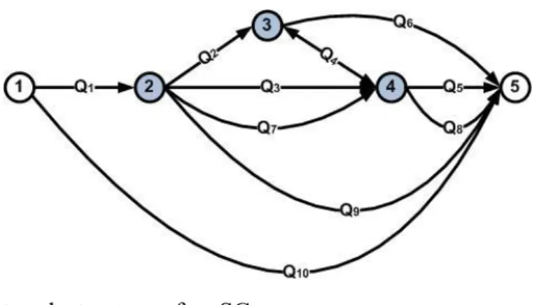
In Fig. 2, the monotonous network structure of an SC is depicted.
Fig. 2. Monotonous network structure of an SC
The simplified SC in Fig. 2 comprises five nodes (nodes #1 and #5 are source and target respec-tively) and ten arcs. For the situation, where disruption may happen only on the arcs, the genome of this SCD includes 11 elements. If disruptions would also be considered for nodes, the genome would include 16 elements. For simplification of the explanation we assume that the nodes are reliable and the failures are subject to the arcs only. In this case, for the given SCD there are five minimum failure edge-cuts as follows (Eq. 2):
1 1 10 2 2 3 7 9 10 3 3 4 6 7 9 10 4 5 6 8 9 10 5 2 4 5 8 9 10 { , }, { , , , , }, { , , , , , }, { , , , , }, { , , , , , } R Q Q R Q Q Q Q Q R Q Q Q Q Q Q R Q Q Q Q Q R Q Q Q Q Q Q (2)
The failure polynomial for this SCD can be represented as follows (Eq.3): 1 2 10 1 10 2 3 7 9 10 3 4 6 7 9 10 5 6 8 9 10 2 4 5 8 9 10 1 2 3 7 9 10 1 3 4 6 7 9 10 1 5 6 8 9 10 1 2 4 5 8 9 10 2 3 4 6 7 9 10 2 3 5 6 7 8 9 10 2 3 4 5 7 8 9 10 3 4 5 6 7 8 ( , ,..., ) T Q Q Q Q Q Q Q Q Q Q Q Q Q Q Q Q Q Q Q Q Q Q Q Q Q Q Q Q Q Q Q Q Q Q Q Q Q Q Q Q Q Q Q Q Q Q Q Q Q Q Q Q Q Q Q Q Q Q Q Q Q Q Q Q Q Q Q Q Q Q Q Q Q Q Q Q Q Q Q Q Q Q Q 9 10 2 4 5 6 8 9 10 1 2 3 4 6 7 9 10 1 2 3 5 6 7 8 9 10 1 2 3 4 5 7 8 9 10 1 3 4 5 6 7 8 9 10 1 2 4 5 6 8 9 10 2 3 4 5 6 7 8 9 10 2 3 4 5 6 7 8 9 10 1 2 3 4 5 6 7 8 9 10 1 2 3 4 5 6 7 8 9 10 Q Q Q Q Q Q Q Q Q Q Q Q Q Q Q Q Q Q Q Q Q Q Q Q Q Q Q Q Q Q Q Q Q Q Q Q Q Q Q Q Q Q Q Q Q Q Q Q Q Q Q Q Q Q Q Q Q Q Q Q Q Q Q Q Q Q Q Q Q Q Q Q Q Q Q Q Q Q Q Q Q Q Q Q Q Q Q Q Q (3)
or in a more compact form as Eq. (4):
2 5 7 8 9 10
( ) 2 4 5 2 .
T Q Q Q Q Q Q Q (4)
In the example in Fig. 2, we have m=5, number of combinations from m for t (t=1,2,3,4,5; i.e., the combination number for 1,2,3,4 and 5 edge-cuts from five minimum edge-cuts) equals 5,10,10,5,1 respectively, n=10 edges. The first five members in T Q Q( ,1 2,...,Q10) (Eq. 3) corre-spond to t=1 (i.e., the edge-cuts from five minimum edge-cuts). Next nine members in Eq. (3) with “-“ are related to t=2 (there should be ten members but one member is cancelled by “+” in t=3). Next seven members with “-“ are related to t=3 (there should be ten members but one member is cancelled by “-” in t=2 and two members are cancelled by “-” in t=4 ). Finally, the last two members with “-“ relate to t=4 (there should be five members but two members are can-celled by “+” in t=3 and one member is cancan-celled by “+” in t=5 ). The genome of this SCD is
(0, 0,1, 0,0, 2, 0, 4, 1,5, 2)
.The interpretation of this genome is as follows:
- The SCD contains 10 transportation edges (vector dimensionality is 11=10+1)
- The components of the genome change their operators (“+” and “-“) three times. This means we have three production sites in the SC (vertices #2, #3 and #4). Node #1 is a supplier, and node #5 is a customer
- The last genome component is “-2”. This means, that the graph has an edge to ensure the direct and return deliveries (i.e., the edge Q4 is a “bridge” that makes it possible to deliv-er products from node #3 to # 4 and return the trucks from #4)
- The first non-zero genome component “1” is the third one. This means that the SCD has one edge combination that contains two edges the failure of which would result in full SC destruction (i.e., the edges { ,Q Q1 10}).
- The second non-zero component is “2” and it is the sixth genome component. This means that the SCD has two edge combinations each of which contains five edges the failure of which would result in full SC destruction (i.e., {Q Q Q Q Q2, 3, 7, 9, 10} and
5 6 8 9 10
Insight 1. The usage of minimum structure failure edge-cuts allows identifying groups of critical suppliers or a critical supplier whose failure separates the network into two disconnected parts and interrupts the SC operation. For SC elements at the minimum structure failure edge-cuts, back-up sourcing strategies need to be implemented.
Furthermore, the genome encompasses the following properties of the monotonous and non-monotonous structures:
if 0 0 and 12...n 1 then the failure polynomial
2
0 1 2
( ) ... n n
T Q Q Q Q describes the monotonous structure;
if 0 and 1 12...n , then the structure is monotonous and for the failure poly-0 nomial is true T(0) 1 and (1)T ; 0
if 0 and 0 12...n , then the structure is non-monotonous and for the failure 0 polynomial is true T(1) ; 0
if0 and 1 12...n , then the structure is non-monotonous and for the failure 1 polynomial is true T(0) 1 .
In addition, the following topological properties of the monotonous structures are contained in the genome:
the power of the lower polynomial member is equal to the minimal power among minimum structure failure edge-cuts (i.e., the number of the first non-zero genome component with
0 0,
l è i i l
); the coefficient of the lower polynomial member is always positive
and equals the number of the minimal-power minimum failure edge-cuts (i.e.,
0 0,
l è i i l
);
the power of the highest polynomial member is equal to the number of the network ele-ments.
The genome can be used for computing the structure failure probability for both monotonous and non-monotonous structures taking into account both homogenous (Fhom) and heterogeneous (Fhet) failure probabilities and possible (Fpossib) failures according to Eq. (5):
1 1 1 ( ) (1, , ,..., ) 2 3 1 T hom F n , 2 1 1 1 ( ) (1, , ,..., ) 2 2 2 T het n F , 2 [0,1] ( ) sup min{ (1, , ,..., n T) , ( )} possib F g . (5)
In the case of homogenous failure probabilities, the network failure probability for the polyno-mial T Q( )01Q2Q2...nQn is in the interval [0,1]. The closer the failure function to
the line T Q , the lower is the network reliability. This property allows using Eq. (6) for ( ) 1 computing the indicator of the network structure failure:
1 1 2 0 1 2 0 1 2 0 0 1 1 1 ( ) ( ) ( ... ) ( , , ,..., ) (1, , ,..., ) 2 3 1 n T hom n n F T Q dQ Q Q Q dQ n
. (6)For heterogeneous failure probabilities, Eq. (7) is used:
1 1 1 1 2 1 2 0 1 2 2 0 0 0 1 1 1 ( ) ... ( , ,..., ) ... ( , , ,..., ) (1, , ,..., ) 2 2 2 T het n n n n F
T Q Q Q dQ dQ dQ . (7) However as pointed out in recent literature (Lim et al. 2014, Simchi-Levi et al. 2014), the usage of failure probabilities in SCD decisions is quite restrictive. Such estimations can be problematic if not enough statistical data is available to fairly estimate the failure probabilities. For this rea-son, the alternative approach can be the usage of the fuzzy-method based on the fuzzy possibility space (Singer 1990).The fuzzy possibility space can be described as ( , ( ), )X X P , where X is a set of elementary
events, ( )X is σ-algebra of subsets in the spaceX , called the events, and the functions
: ( ) [0,1]
P X , called the possibility measure (i.e., P A is the possibility of the event( ) ( )
A X ). The event possibility is defined by the possibility distribution functiong X : [0,1]
as ( ) sup ( )
x A
P A g x
. In the possibility measure space, the fuzzy element ( ) ( : X [0,1])
is defined. Its membership function can be described as the possibility distribution function
( )x P x( ) g x( ), x X
.
Further assume that the SC network structure comprises i i( ), i1, 2,...,n fuzzy elements. Using the operators for fuzzy structures (12 12 1 2, 12 1 2), the struc-ture failure possibility polynomial with homogenous fuzzy elements (12 ...n :) can be described asT( ) 0 1 2 2... n n, where ( 0, 1, 2,...,n)is the structure genome.
Similar to the probabilistic approach, we consider the computational procedure for the indicator of the network structure failure. According to reliability theory, in the function classL X a pos-( ) sibility measure integral is defined in (Pyt’ev 2002). The function classL X includes the func-( ) tions f X: L, whereL ([0, 1], , , ) is the possibility value scale in the interval [0, 1] ,
sub-ject to operators , «+» and « »:a b max{ , }a b anda b min{ , }a b ). These functions en-compass the following properties:
1. [0,1], f L X( ) f L X( ).
2. f L X( ),v:[0,1][0,1]are the involutions of the monotonously decreasing function
(0) 1, (1) 0 v v )v f v f x( ( ))L X( )(Pyt’ev 2002). 3. fi L X( ),i1, 2,.... 1 i( ) sup ( )i ( ), 1 i( ) inf i( ) ( ) i f x i f x L X i f x i f x L X .
Integralp L X: ( )Lfor the possibility measure ( ) sup ( )
x A
P A g x
at the distribution g is defined
as: ( ) sup min{ ( ), ( )}
x X
p f f x g x
. If the possibility measure is defined by the distribution
( )
gL X , then the following is true (Eq. 8):
[0,1] [0,1]
[0,1] ( ) 0
( )
( ) sup min{ , ({ ( ) })} sup min{ ,sup{ ( ) ( ) }}
sup sup min{ , ( )} sup sup min{ , ( )} sup min{ ( ), ( )} ( ).
x X x X x X f x x X f x s f P x f x g x f x g x g x f x g x p f (8),
where s f( )is classical Sugeno fuzzy integral (Sugeno 1974).
The polynomial of the structure failure possibility T( ) 0 1 2 2... n nis always
bounded as 0T( ) 1 . For monotonous structures ( )T , T(0)0, T(1) 1 also increases mo-notonously. For non-monotonous structures, the polynomial of the structure failure possibility is eitherT(0) 1 or (1)T ), or ( (0) 1,0 T T(1)0). Since the polynomial of the structure failure possibility is a functionT:[0,1]L, it belongs to the classL([0, 1]).
This property allows using as an integral indicator of the structure failure possibility the integral for the possibility measure (Eq. 9) and provides evidence for structure failure probabilities de-fined in Eq. (5):
2
[0,1] [0,1]
( ) sup min{ ( ), ( )} sup min{ (1, , ,..., n T) , ( )}
possib F T g g . (9)
5. Modelling the SC structure dynamics with reconfiguration
As a consequence of a disruption, a SCD can have the form of different states S. A state repre-sents the SCD (i.e., the graph G=(V,E)) subject to non-disrupted and disrupted elements. Due to the fact that the SC elements can recover after a failure it should be noted that the initial state S0 denotes the state where no SC element is failing. Subsequently, due to disruptions and recovery
actions, the SCD graph can transit through different states. An example for five state levels is given in Fig. 3.
Fig. 3. Levels of the SC structure dynamics
The first degradation level corresponds to those states with the failure in one element; the second degradation level corresponds to the states with the failure in two elements, etc. The recovery actions move the SCD back from the second level to the first level, and so on. The sequence of the transitions through the structural states is called SC structure dynamics control (Ivanov et al. 2010, Ivanov and Sokolov 2012). The sequence of events for the structure dynamics is called the
structure dynamics scenario.
Scenarios belong to crucial issues in the SCD resilience analysis. In general, we do not know exactly which elements will fail. However, the structure failure polynomial (Eqs 1 and 2) con-tains the graph structure. For example, in the case of Q1 failure, we have an indirect failure of Q2,Q3,Q4,Q5,Q6,Q7,Q8, and Q9. In other words, the SCD will transit in a state where Q1,Q2,Q3,Q4,Q5,Q6,Q7,Q8, and Q9 are missing.
In addition, failures in different elements may have different impact on the SCD resilience. That is why we suggest analyzing homogenous, heterogeneous and possibilistic failures, respectively. Finally, recovery actions may influence the resilience. That is why we suggest considering three scenarios, i.e., worst case (failure in the most critical elements and no recovery measures), aver-age case and no reconfiguration, and averaver-age case with reconfiguration (see Sect. 6).
Since genome represents the SCD, each structural state Scan be described by a genome. Therefore, the total resilience or total failure of a path in the SC structure dynamics can be
com-puted using Eqs (6), (7) and (9). With the help of integrating these indicators, SCD resilience can be quantified for homogenous, heterogeneous and possibilistic failures and recovery actions.
Consider the SC reconfiguration processes. Denote as Qj
the transition from one
struc-tural state S (described as a genome ) to another structural state S(described as a genome) as a consequence of a failure/recovery in a graph elementQjQˆ. Denote as X( ) the set of all structural states subject to . Then, a reconfiguration scenario in the degradation or recovery process subject to an initial stateS and the state0 S can be described as the following transition f
chain (Eq. 10): 3 1 1 2 0 1 2 ... 1 , j j j j j N N N N Q Q Q Q Q (10) where 0 0, N f , 1 2 ˆ { , ,..., } N j j j Q Q Q Q
The structural changes in the intermediate states on the reconfiguration path will be described as structural failure indicatorFfailure() { Fhom(),Fhet (),Fpossib ()}. Then the problem of optimistic structure reconfiguration path ((i.e., the case where recovery actions are included) can be described as the following optimization problem (11):
0 1 1 2 0 0 ( ) , , ( ) , ˆ { , ,..., } . j N j j N N failure j f j j j minimize F subject to X Q Q Q Q
(11)To solve the problem (11), a hybrid branch-and-bound/evolutionary algorithm has been devel-oped as follows.
Step 1. At each k -iteration, a random sequence is built
0 1 2 1 ( ) ( ) ( ) ( ) , , , ..., , N N k k k k (where 0 0, N f
) that corresponds to a structure reconfiguration path.
Step 2. For the structure reconfiguration path, the indicator
1 ( ) ( ) 1 ( ) ( ) j N k k failure failure j F F
iscom-puted. The random transition to an intermediate state subject to genome ( ) j
k
is modeled accord-ing to normal distribution.
Step 3. The value of
1 ( ) ( ) 1 ( ) ( ) j N k k failure failure j F F
for the structure reconfiguration path iscom-pared with the F-value at k-1 iteration.
The problem of pessimistic structure dynamics path (i.e., the case where no recovery actions are included) can be described as the following optimization problem (12):
0 1 1 2 0 0 ( ) , , ( ) , ˆ { , ,..., } . j N j j N N failure j f j j j maximize F subject to X Q Q Q Q
(12)6. Development of the SC design resilience index
In Fig. 4, a path
( )k of SC structure reconfiguration is shown.Fig. 4. Supply chain structure reconfiguration path
The area
S
k equals ( )0,1,..., min { ( )} j k failure j N F N
and describes the total structural resilience for a given reconfiguration path by holding the structure failure values during the reconfiguration. The
computed area 1 ( ) ( ) 1 0 0 ( ) ( ) 2 j j k k N failure failure k j F F S
describes the total structural resilience for agiven reconfiguration path by changes in the structure failure values during the reconfiguration on the path
( )k . In this case, the relation (Eq. 13) describes the SCD resilience during the struc-tural reconfiguration on the path
( )k0 k k k S J S (13)
max
max{ k}
k
J J corresponds to the optimistic scenario, and min
min{ k}
k
J J corresponds to the
pessimistic scenario.
Consider M experiments. At each
k
-experiment, the sequence0 1 2 1 ( ) ( ) ( ) ( )
,
,
, ...,
,
N N k k k k
(where
0
0, N
f ) is built according to a SCDstructure reconfiguration path. For the path, the value of 0
k k k S J S
is computed. Finally, the
average of all experiments is computed as shown in Eq. (14).
0 1
1
M k kJ
J
M
(14)The SCD structure resilience
J
SU belongs to the interval [J
min,J
max] and the expected SC resilience isJ
0. The values ofJ
SU can be described as a fuzzy triple (a
, ,
), whereaJ0,0 min
J J
,
JmaxJ0.Considering three cases (monotonous structure, non-monotonous structure and structure with possible failures), three fuzzy triples are computed (
a
î,
î,
î ), (a
n,
n,
n), (a
,
,
). Then the integral SCD structure resilienceJ
SU is computed as Eq. (15):( , , ) ( , , ) ( , , ) ( , , ) 3 î î î n n n SU a a a J a (15)
Finally, the center-of-gravity method is used to avoid the fuzziness in the final solution (Eq. 16):
( ) 3 SU E J a . (16)
3 2 1 5 6 7 4 9 11 10 12 8 8 3 2 1 5 6 7 4 9 11 10 12 1 2 5 6 7 4 9 10 11 12 8 3 7. Experimental results
For analysis, we consider four SC network structures from the study by Kim et al. (2015) (Fig. 5).
a) b)
c) d)
Fig. 5. References SC network structures
In terms of the probabilistic-fuzzy approach, these structures are represented as shown in Fig. 6.
structure a): structure b):
3 2 1 5 6 7 8 4 9 11 10 12
structure c): structure d):
Fig. 6. Modified representation of the referenced SC network structures
In Fig. 6, the SC nodes are marked grey and SC arcs are marked white. The node #1 is target and the node #12 is source. For example for the structure (a), the failure polynomial can be repre-sented as follows (note that Q=1-P):
T(P, Q) = P30 P27 P26 Q25 P24 Q23 Q22 P15 P8 P7 P6 P5 + + P30 P25 P24 Q22 P15 P8 P6 P5 + + P30 P26 P23 Q22 P15 P8 P7 P5 + + P29 P21 P20 Q19 P14 P11 P10 P9 + + P28 P18 Q17 P16 P13 P4 P3 P2 + + P30 P22 P15 P8 P5 + + P29 P19 P14 P11 P9 + + P28 P17 P13 P4 P2 - - P29 P28 P19 P17 P14 P13 P11 P9 P4 P2 - - P30 P29 P22 P19 P15 P14 P11 P9 P8 P5 - - P30 P28 P22 P17 P15 P13 P8 P5 P4 P2 + + P30 P29 P28 P22 P19 P17 P15 P14 P13 P11 P9 P8 P5 P4 P2 - - P30 P28 P22 P18 Q17 P16 P15 P13 P8 P5 P4 P3 P2 - - P29 P28 P19 P18 Q17 P16 P14 P13 P11 P9 P4 P3 P2 + + P30 P29 P28 P22 P19 P18 Q17 P16 P15 P14 P13 P11 P9 P8 P5 P4 P3 P2 - - P29 P28 P21 P20 Q19 P18 Q17 P16 P14 P13 P11 P10 P9 P4 P3 P2 - - P30 P29 P22 P21 P20 Q19 P15 P14 P11 P10 P9 P8 P5 - - P29 P28 P21 P20 Q19 P17 P14 P13 P11 P10 P9 P4 P2 + + P30 P29 P28 P22 P21 P20 Q19 P17 P15 P14 P13 P11 P10 P9 P8 P5 P4 P2 + + P30 P29 P28 P22 P21 P20 Q19 P18 Q17 P16 P15 P14 P13 P11 P10 P9 P8 P5 P4 P3 P2 - - P30 P29 P26 P23 Q22 P21 P20 Q19 P15 P14 P11 P10 P9 P8 P7 P5 - - P30 P28 P26 P23 Q22 P18 Q17 P16 P15 P13 P8 P7 P5 P4 P3 P2 - - P30 P29 P26 P23 Q22 P19 P15 P14 P11 P9 P8 P7 P5 -
- P30 P28 P26 P23 Q22 P17 P15 P13 P8 P7 P5 P4 P2 + + P30 P29 P28 P26 P23 Q22 P19 P17 P15 P14 P13 P11 P9 P8 P7 P5 P4 P2 + + P30 P29 P28 P26 P23 Q22 P19 P18 Q17 P16 P15 P14 P13 P11 P9 P8 P7 P5 P4 P3 P2 + + P30 P29 P28 P26 P23 Q22 P21 P20 Q19 P18 Q17 P16 P15 P14 P13 P11 P10 P9 P8 P7 P5 P4 P3 P2 + + P30 P29 P28 P26 P23 Q22 P21 P20 Q19 P17 P15 P14 P13 P11 P10 P9 P8 P7 P5 P4 P2 - - P30 P26 P25 P24 P23 Q22 P15 P8 P7 P6 P5 - - P30 P29 P25 P24 Q22 P21 P20 Q19 P15 P14 P11 P10 P9 P8 P6 P5 - - P30 P28 P25 P24 Q22 P18 Q17 P16 P15 P13 P8 P6 P5 P4 P3 P2 - - P30 P29 P25 P24 Q22 P19 P15 P14 P11 P9 P8 P6 P5 - - P30 P28 P25 P24 Q22 P17 P15 P13 P8 P6 P5 P4 P2 + + P30 P29 P28 P25 P24 Q22 P19 P17 P15 P14 P13 P11 P9 P8 P6 P5 P4 P2 + + P30 P29 P28 P25 P24 Q22 P19 P18 Q17 P16 P15 P14 P13 P11 P9 P8 P6 P5 P4 P3 P2 + + P30 P29 P28 P25 P24 Q22 P21 P20 Q19 P18 Q17 P16 P15 P14 P13 P11 P10 P9 P8 P6 P5 P4 P3 P2 + + P30 P29 P28 P25 P24 Q22 P21 P20 Q19 P17 P15 P14 P13 P11 P10 P9 P8 P6 P5 P4 P2 + + P30 P29 P26 P25 P24 P23 Q22 P21 P20 Q19 P15 P14 P11 P10 P9 P8 P7 P6 P5 + + P30 P28 P26 P25 P24 P23 Q22 P18 Q17 P16 P15 P13 P8 P7 P6 P5 P4 P3 P2 + + P30 P29 P26 P25 P24 P23 Q22 P19 P15 P14 P11 P9 P8 P7 P6 P5 + + P30 P28 P26 P25 P24 P23 Q22 P17 P15 P13 P8 P7 P6 P5 P4 P2 - - P30 P29 P28 P26 P25 P24 P23 Q22 P19 P17 P15 P14 P13 P11 P9 P8 P7 P6 P5 P4 P2 - - P30 P29 P28 P26 P25 P24 P23 Q22 P19 P18 Q17 P16 P15 P14 P13 P11 P9 P8 P7 P6 P5 P4 P3 P2 - - P30 P29 P28 P26 P25 P24 P23 Q22 P21 P20 Q19 P18 Q17 P16 P15 P14 P13 P11 P10 P9P8P7P6P5P4P3P2 - - P30 P29 P28 P26 P25 P24 P23 Q22 P21 P20 Q19 P17 P15 P14 P13 P11 P10 P9 P8 P7 P6 P5 P4 P2 - - P30 P29 P27 P26 Q25 P24 Q23 Q22 P21 P20 Q19 P15 P14 P11 P10 P9 P8 P7 P6 P5 - - P30 P28 P27 P26 Q25 P24 Q23 Q22 P18 Q17 P16 P15 P13 P8 P7 P6 P5 P4 P3 P2 - - P30 P29 P27 P26 Q25 P24 Q23 Q22 P19 P15 P14 P11 P9 P8 P7 P6 P5 - - P30 P28 P27 P26 Q25 P24 Q23 Q22 P17 P15 P13 P8 P7 P6 P5 P4 P2 + + P30 P29 P28 P27 P26 Q25 P24 Q23 Q22 P19 P17 P15 P14 P13 P11 P9 P8 P7 P6 P5 P4 P2 + + P30 P29 P28 P27 P26 Q25 P24 Q23 Q22 P19 P18 Q17 P16 P15 P14 P13 P11 P9 P8 P7 P6 P5 P4 P3 P2 + + P30 P29 P28 P27 P26 Q25 P24 Q23 Q22 P21P20Q19 P18Q17P16P15P14P13P11P10P9P8P7P6P5P4P3P2 + + P30 P29 P28 P27 P26 Q25 P24 Q23 Q22 P21 P20 Q19 P17 P15 P14 P13 P11 P10 P9 P8 P7 P6 P5 P4 P2
According to the model and algorithm in Sect. 5, the modelling of the worst case (failure in the most critical elements and no recovery measures), average case and no reconfiguration, and av-erage case with reconfiguration subject to both nodes and arcs failures has been performed. Simi-lar to Kim et al. (2015), we assumed that the node #1 (Target) and node #12 (Source) are not perturbed. The computed values of SCD resilience are presented in Table 1.
Table 1 Computed values of SCD resilience
Structure SCD structural resilience
SU
J
Worst-case (no reconfiguration) Average case (no reconfiguration) Average case (with reconfiguration)(
SU)
E J
a 0.0615 0.1548 0.7056 0.3073 b 0.0496 0.2538 0.8606 0.3880 c 0.0289 0.2527 0.8306 0.3707 d 0.0456 0.1640 0.7519 0.3205In Table 2, the results are compared with the resilience estimation from Kim et al. (2015).
Table 2 Comparison of the values of SCD resilience
Structure Resilience values
Kim et al. (2015) Our approach
(with reconfigu-ration)
Our approach (no reconfiguration)
a 0.11 0.31 0.15
b 0.30 0.39 0.25
c 0.16 0.37 0.25
d 0.13 0.32 0.16
In comparing the results of these methods, it can be observed that all methods suggest the same order of the resilient SCD: BCDA. At the same time, the difference in the absolute resili-ence values can be observed in comparing the results of Kim et al. (2015), our results without reconfiguration and our results with reconfiguration. Besides, in the study by Kim et al. (2015), the SCD #B has a significantly higher resilience as compared to three other structures. In our analysis, the resilience of B and C is close to each other. The explanation of these effects can be seen in the inclusion of the reconfiguration and fuzzy-probabilistic analysis into resilience index computation.
Insight 2. SC resilience depend both on network structure characteristics and recovery policies. Fair SC resilience estimation needs to include both proactive and reactive policies in order to compare different SCDs regarding the resilience. For SC elements at the minimum structure failure edge-cuts, proactive strategies need to be integrated with recovery policies.
In addition, the inclusion of the minimum edge-cut failures in the genome (instead of individual failures in the reliability analysis) is seen as the explanation of the effects in computational re-sults. This is the benefit and novelty of the proposed approach. It can also be observed that ex-cept for structure (b), the difference of the values of Kim et al. (2015) and our results in the case with reconfiguration is approximately 0.2. The reason for this phenomenon is, on one hand, the inclusion of the pessimistic scenario (i.e., worst-case and no recovery actions) into our resilience index. Additionally, similarities in failures (to ensure the comparativeness of the results) lead to such a correlation. Finally, higher resilience values in our approach can be observed. If compar-ing the results of our approach with and without reconfiguration, it can be noted that the pro-posed method to compute structure resilience index works in both cases. Its values also reflect clearly that the inclusion of reconfiguration increases the SCD resilience. This insight requires more analysis efforts subject to different recovery policies but we can assume the effect of the SC structure reconfiguration as resilience increase driver.
8. Managerial Insights
Disruption risks may result into ripple effect and structure dynamics in the SC. It is to notice that the scope of the rippling and its performance impact depend both on robustness reserves (e.g., redundancies like inventory or capacity buffers) and speed and scale of recovery actions (Knemeyer et al. 2009, Hu et al. 2013, Ivanov and Sokolov 2013, Kim and Tomlin, 2013, Pettit et al. 2013). In many practical settings, companies need analysis tools to estimate both the SC efficiency and SC resilience. For SC resilience, the impacts of recovery actions subject to differ-ent disruptions and performance indicators need to be estimated.
The results of this study contribute to support decisions in these practical problems. The devel-oped model can help the SC risk managers to identify whether the existing SCD is resilient for different disruption scenarios. The model also considers mitigation strategies (i.e., reconfigura-tion) that can be used by SC risk managers and translated into the SCD changes.
With the use of the developed approach, SC managers can compare different possible SCDs re-garding their resilience using the proposed SCD resilience index. Since the calculation of the resilience index includes the recovery actions, the developed model can help to identify opportu-nities to reduce disruption and recovery costs by SC re-design. If the experts can forecast or at least assume possible failures and recovery actions, it becomes possible to create reconfiguration scenarios (see. Fig. 4) and compute the SCD resilience index subject to optimistic, pessimistic or possibility failure scenarios.
critical supplier whose failure interrupts the SC operation fully. The identification of such critical suppliers with the help of genome analysis and minimum edge-cuts usage may allow re-designing the SC in order to increase the SCD resilience without efficiency decrease. In addition, the identification of nodes and arcs in the minimum edge-cuts in the SC the failure of which is critical for SCD survivability may help to develop more specific risk mitigation policies such as dual sourcing or continuous risk monitoring.
With the help of the structure dynamics control, the model analyses effective ways to recover and re-allocate resources and flows after the disruption. The model can be used by SC risk spe-cialists to adjust mitigation and recovery policies with regard to critical SCD elements. Finally, the usage of the fuzzy-probabilistic approach extends possible application of the developed method regarding the data availability for analysis.
9. Conclusions
In recent literature, SCD models have been extensively considered in the light of severe disrup-tions. SC resilience became one of the key investigation categories. The existing graph-theoretical studies have mostly focused on the impact of disruptions on SCD resilience using the reliability theory without considering structure reconfiguration. In this paper, we take another perspective and extend the existing models to SCD resilience analysis by incorporating the struc-ture reconfiguration. In the scope of this research is the analysis of what SC elements will sur-vive (i.e., be in operation) after a disruption and under which conditions (i.e., failure in a group of suppliers that interrupt the SC operation fully) the SC can still survive or it will lose its resili-ence.
The research methodology is based on a hybrid fuzzy-probabilistic approach to network resil-ience analysis. The SCD resilresil-ience analysis is performed as the analysis of optimistic, pessimis-tic, and random (possible) reconfiguration paths of an SC structure due to disruptions. The appli-cation of the developed structure resilience index is demonstrated by the computation on the ref-erenced SCD examples from the literature.
The results have some major implications. First, it suggests a method to compare different SCDs regarding the resilience. Second, since the reconfiguration is included, the resilience analysis becomes more realistic and considers both disruptions and recovery. Third, the developed method can be used both for monotonous and non-monotonous structures. Fourth, the usage of minimum structure failure edge-cuts allows identifying groups of critical suppliers or a critical supplier whose failure separates the network into two disconnected parts and interrupts the SC operation fully.
In future, the gained insights require more detailed analysis efforts regarding the effect of the SCD structure reconfiguration as resilience increase driver. It is a very important task to develop methods of how to restore the SCD structure from an available genome. This task is quite similar to inverse problems in linear programming. In addition, the complexity issue in genome calcula-tion (e.g., for structure C, the polynomial contains over 3,000 elements) needs to be addressed based on the development of efficient heuristic methods. Finally, development of risk mitigation policies for critical suppliers at the minimum edge-cuts is an interesting future research avenue.
References
Aggarwal, K.K., J.S. Gupta, & R.B. Misra (1973). A New Method for System Reliability Evaluation. Microelectronics and Reliability, 12, 435-440.
Ambulkar, S., Blackhurst, J., & Grawe, S. (2015). Firm's resilience to supply chain disruptions: Scale development and empirical examination. Journal of Operations Management, 33(34), 111–122.
Bakshi, N., & Kleindorfer, P.R. (2009). Co-opetition and investment for supply-chain resilience. Produc-tion and OperaProduc-tions Management, 18(6), 583–603.
Brandon-Jones, E., Squire B., & Van Rossenberg, Y.G.T. (2015). The impact of supply base complexity on disruptions and performance: the moderating effects of slack and visibility. International Journal of Production Research, 53(22), 6903-6918.
Bode, C., & Wagner, S. M. (2015). Structural drivers of upstream supply chain complexity and the fre-quency of supply chain disruptions. Journal of Operations Management 36, 215-228.
Colbourn C.J. (1987). The combinatorics of network reliability. New York: Oxford University Press. Das K. & Lashkari R.S. (2015). Risk readiness and resiliency planning for a supply chain. International
Journal of Production Research, 53(22), 6752-6771. Deistel, R. (2012). Graph Theory. Springer, 4th Ed.
Dolgui, A., and Proth, J.-M. (2010) Supply chain engineering: useful methods and techniques, Springer. Garvey, M.D., Carnovale S., Yeniyurt, S. (2014). Analytical framework for supply network risk
propaga-tion: A Bayesian network approach. European Journal of Operational Research, 243, 618–627. Gunasekaran A., Subramanian N. & Rahman S. (2015). Supply chain resilience: role of complexities and
strategies. International Journal of Production Research, 53(22), 6809-6819.
Han, J., & Shin, K.S. (2016). Evaluation mechanism for structural robustness of supply chain considering disruption propagation. International Journal of Production Research, 54(1), 135-151.
Hsu, C.I., & Li, H.C. (2011). Reliability evaluation and adjustment of supply chain network design with demand fluctuations. International Journal of Production Economics, 132(1), 131–145.
Hu, X, Gurnani, H., & Wang, L. (2013). Managing risk of supply disruptions: Incentives for capacity restoration. Production and Operations Management, 22(1), 137–150.
Ivanov D, Sokolov B., & Kaeschel J. (2010). A multi-structural framework for adaptive supply chain planning and operations with structure dynamics considerations. European Journal of Operational Re-search, 200, 409–420.
Ivanov D., & Sokolov B. (2013). Control and system-theoretic identification of the supply chain dynam-ics domain for planning, analysis, and adaptation of performance under uncertainty. European Journal of Operational Research, 224(2), 313–323.
Ivanov D., & Sokolov B. (2012). Structure dynamics control approach to supply chain planning and adap-tation, International Journal of Production Research, 50(21), 6133-6149.
Ivanov D., Sokolov B., & Pavlov, A. (2013). Dual problem formulation and its application to optimal re-design of an integrated production–distribution network with structure dynamics and ripple effect con-siderations. International Journal of Production Research, 51(18), 5386–5403.
Ivanov, D., Sokolov, B., & Dolgui, A. (2014а). The ripple effect in supply chains: Trade-off ‘efficiency-flexibility-resilience’ in disruption management. International Journal of Production Research, 52(7), 2154–2172.
Ivanov, D., Sokolov, B., & Pavlov, A. (2014b). Optimal distribution (re)planning in a centralized multi-stage network under conditions of ripple effect and structure dynamics. European Journal of Opera-tional Research, 237(2), 758–770.
Ivanov D., Sokolov B., Pavlov A., Dolgui A., & Pavlov D. (2016). Disruption-driven supply chain (re)-planning and performance impact assessment with consideration of pro-active and recovery policies, Transportation Research: Part E, in press.
Kamalahmadi M., Mellat-Parast M.M. (2016a). A review of the literature on the principles of enterprise and supply chain resilience: Major findings and directions for future research. Int. Journal of Produc-tion Economics, 171, 116–133.
Kamalahmadi M. & Mellat-Parast M. (2016b). Developing a resilient supply chain through supplier flex-ibility and reliability assessment. International Journal of Production Research, 54(1), 302-321.
Khakzad, N. (2015). Application of dynamic Bayesian network to risk analysis of domino effects in chemical infrastructures. Reliability Engineering and System Safety, 138, 263-272.
Kim, S.H., & Tomlin, B. (2013). Guilt by association: Strategic failure prevention and recovery capacity investments. Management Science, 59(7), 1631–1649.
Kim, Y., Chen Y.-S., & Linderman, K. (2015). Supply network disruption and resilience: A network structural perspective. Journal of Operations Management, 33–34, 43–59.
Kopytov E.A., Pavlov A.N., & Zelentsov V.A. (2010). New methods of calculating the Genome of struc-ture and the failure criticality of the complex objects’ elements. Transport and Telecommunication, 11(4), pp. 4-13.
Liberatore F, Scaparra M.P., & Daskin M.S. (2012). Hedging against disruptions with ripple effects in location analysis. Omega 40, 21–30.
Lin, Y.K., Huang, C.F., & Yeh, C.T. (2014). Network reliability with deteriorating product and produc-tion capacity through a multi-state delivery network. Internaproduc-tional Journal of Producproduc-tion Research, 52(22), 6681–6694.
Munoz A. & Dunbar M. (2015). On the quantification of operational supply chain resilience. International Journal of Production Research, 53(22), 6736-6751.
Nair, A. & Vidal, J.M. (2010). Supply network topology and robustness against disruptions – An investi-gation using a multi-agent model. International Journal of Production Research, 49(5), 1391–1404. Pettit, T.J., Croxton, K.L. & Fiksel, J. (2013). Ensuring supply chain resilience: Development and
imple-mentation of an assessment tool. Journal of Business Logistics, 34(1), 46–76.
Pyt’ev Yu.P. (2002). The Methods of the Possibility Theory in the Problems of Optimal Estimation and Decision Making: VI. Fussy Sets. Independence. P-Complection.Methods for Estimation Fuzzy Sets and Their Parameters. Pattern Recognition and Image Analysis, 12(2),107–115.
Ryabinin I.A. (1976). Reliability of Engineering Systems. Principles and Analysis. Mir, Moscow.
Schoenlein, M., Makuschewitz, T., Wirth, F., & Scholz-Reiter, B. (2013). Measurement and optimization of robust stability of multiclass queuing networks: Applications in dynamic supply chains. European Journal of Operational Research, 229, 179–189.
Sheffi, Y., & Rice, J.B. (2005). A supply chain view of the resilient enterprise. MIT Sloan Management Review, 47(1), 41–48.
Simchi-Levi, D., Schmidt, W., & Wei, Y. (2014). From superstorms to factory fires: Managing unpredict-able supply chain disruptions. Havard Business Review, February.
Singer D. (1990). A fuzzy set approach to fault tree and reliability analysis. Fuzzy Sets and Systems, 34(2), 145-155.
Snyder, L V., Zümbül A., Peng P., Ying R., A. J. Schmitt, and B. Sinsoysal (2016). OR/MS Models for Supply Chain Disruptions: A Review. IIE Transactions, 48(2), 89-109.
Sokolov, B., Ivanov, D., Dolgui, A., & Pavlov, A. (2016). Structural analysis of the ripple effect in the supply chain. International Journal of Production Research, 54(1), 152-169.
Soni, U., Jain, V., & Kumar, S. (2014). Measuring supply chain resilience using a deterministic modeling approach. Computers & Industrial Engineering, 74, 11–25.
Sugeno, M. (1974). Theory of fuzzy integrals and its applications: Ph.D. Thesis, Tokyo.
Tang, L., Jing K., He J., Stanley, H.E. (2016). Complex interdependent supply chain networks: Cascading failure and robustness. Physica A, 443, 58–69.
Wagner, S.M., & Neshat, N. (2010). Assessing the vulnerability of supply chains using graph theory. International Journal of Production Economics, 126 (1), 121-129.
Wang, D., & Ip, W.H. (2009). Evaluation and analysis of logistic network resilience with application to aircraft servicing. IEEE Systems Journal, 3, 166–173.
Wierczek, A. (2014). The impact of supply chain integration on the "snowball effect" in the transmission of disruptions: An empirical evaluation of the model. International Journal of Production Economics, 157(1), 89-104.
Wu, T., Blackhurst, J., & O’Grady, P. (2007). Methodology for supply chain disruption analysis. Interna-tional Journal of Production Research, 45(7), 1665–1682.
Xu, M., Wang, X., & Zhao, L. (2014). Predicted supply chain resilience based on structural evolution against random supply disruptions. International Journal of Systems Science: Operations & Logistics, 1(2), 105–117.
Zobel, C.W., & Khansa, L. (2014). Characterizing multi-event disaster resilience. Computers & Opera-tions Research, 42, 83–94.