HAL Id: hal-01244802
https://hal.inria.fr/hal-01244802
Submitted on 16 Dec 2015
HAL is a multi-disciplinary open access
archive for the deposit and dissemination of
sci-entific research documents, whether they are
pub-lished or not. The documents may come from
teaching and research institutions in France or
abroad, or from public or private research centers.
L’archive ouverte pluridisciplinaire HAL, est
destinée au dépôt et à la diffusion de documents
scientifiques de niveau recherche, publiés ou non,
émanant des établissements d’enseignement et de
recherche français ou étrangers, des laboratoires
publics ou privés.
OA-DVFA: A Distributed Virtual Forces-based
Algorithm to Monitor an Area with Unknown Obstacles
Ines Khoufi, Pascale Minet, Anis Laouiti
To cite this version:
Ines Khoufi, Pascale Minet, Anis Laouiti. OA-DVFA: A Distributed Virtual Forces-based Algorithm
to Monitor an Area with Unknown Obstacles. Consumer Communications & Networking Conference
(CCNC), Jan 2016, Las-Vegas, United States. �hal-01244802�
OA-DVFA: A Distributed Virtual Forces-based
Algorithm to Monitor an Area
with Unknown Obstacles
Ines Khoufi and Pascale Minet
Inria, Rocquencourt, 78153 Le Chesnay Cedex, France.
Email: [email protected] Email: [email protected]
Anis Laouiti
TELECOM SudParis, CNRS Samovar UMR 5157 91011 Evry Cedex, France. Email: [email protected]
Abstract—Deployment of sensor nodes to fully cover an area has caught the interest of many researchers. However, some simplifying assumptions are adopted such as knowledge of obstacles, centralized algorithm... To cope with these drawbacks, we propose OA-DVFA (Obstacles Avoidance Distributed Virtual Forces Algorithm) a self-deployment algorithm to ensure full area coverage and network connectivity. This fully distributed algorithm is based on virtual forces to move sensor nodes. In this paper, we show how to avoid the problem of node oscillations and to detect the end of the deployment in a distributed way. We evaluate the impact of the number, shape and position of obstacles on the coverage rate, the distance traveled by all nodes and the number of active nodes. Simulation results show the very good behavior of OA-DVFA.
I. INTRODUCTION
Area coverage and network connectivity are two major issues in Wireless Sensor Networks (WSNs) to perform the monitoring of the area considered. The goal is to guarantee that each event occurring in this area can be detected by at least one sensor node and there is at least one path to report this detected event to the sink. A sensor node is an entity that has a sensing range (r) which defines the zone where it can detect events and a communication range (R) which determines its radio neighborhood. A sensor node can be static or mobile. In any case, sensor nodes need a deployment algorithm to determine their appropriate positions in order to efficiently monitor the area considered. Deployment algorithms are the focus of many studies. They are various and depend on the entity monitored (area, barrier or point of interest), the required coverage (full, partial), the required network connectivity (permanent, intermittent, k-connectivity) and also the type of sensor nodes (static or mobile). The deployment algorithm can be centralized: a central entity is in charge of computing the position of each node. This requires full knowledge of the area monitored. Otherwise, the deployment algorithm is called self-deployment where mobile and autonomous sensor nodes cooperate with each other to determine their new positions and move to their new positions. Many studies assume that the area considered does not contain obstacles or the obstacles are known. However, in the real environment, obstacles exist and they can be known or unknown. When obstacles are unknown, the deployment algorithm should take into account this constraint and perform a discovery task to detect the
presence of obstacles. In the literature, only few studies take into account the presence of unpredictable obstacles in the area considered. Then, designing a distributed deployment algorithm that deals with unknown obstacles is still a challenge that we propose to tackle in this paper.
II. RELATEDWORK
In the literature, many studies focus on the deployment of wireless sensor nodes in an area containing known obstacles. However, only few studies deal with unknown and unpre-dictable obstacles. This situation corresponds to the require-ment of many applications such as for instance monitoring of a post-disaster area and damage assessment. The deployment of autonomous sensor nodes in an area that may contain unknown obstacle is the focus of this paper.
Among the studies dealing with unknown obstacles, we dis-tinguish two approaches: on the one hand a deployment of static sensor nodes assisted by a mobile robot, and on the other hand a self deployment of autonomous and mobile sensor nodes. The assisted deployment approach is illustrated in [1] and [2]. In [1], the robot follows a spiral movement policy to deploy static sensor nodes along its trajectory in order to ensure full area coverage. Since the authors assume that the area may contain obstacles which are not known by the robot, they propose some movement policies to bypass the obstacles. In a similar context, authors in [2], propose a serpentine movement policy with obstacle handling policy and boundary policy. The robot has to follow the serpentine movement policy while placing static sensor nodes separated by the optimal distance to reduce the total number of sensor nodes. Both methods proposed in [1] and [2], provide full coverage using the minimum number of sensor nodes.
Concerning self-deployment approach, the authors in [3] pro-pose a Self-deployment Obstacles Avoidance (SOA) algorithm that ensures coverage and connectivity between the sink and a target. The position of the target is known by all sensor nodes initially grouped around the sink. Some rules and priorities are proposed to move sensor nodes toward the target establishing n parallel routes. Sensor nodes are grouped in n-tuples. The n-tuple with the highest priority is the leader. It computes the trajectory to the target and avoids obstacles when detected. To reduce the computation cost, the remaining n-tuples follow the trajectory of the leader n-tuple. A high value of n increases
the coverage rate of the area considered surrounding the sink and the target. This principle is dedicated to ensure a reliable coverage and connectivity between the sink and the target. This work differs from our study that aims to ensure full area coverage and network connectivity in an unknown environment.
More studies exist about self-deployment. Since the virtual forces principle can be easily applied in a distributed way, it is largely adopted in self-deployment of sensor nodes. More precisely, virtual forces work as follows.
The virtual force based strategy is based on virtual forces that make sensors move. Each sensor node exerts an attractive or repulsive force on each of its neighbors. This force depends on the distance between the sensor node considered and its neighbor. The goal is to reach a predefined target distance. The force exerted is attractive if the distance between two neighboring nodes is higher than the target distance and it is repulsive if the distance between two neighboring nodes is less than the target distance. Otherwise, the force is null. Let us
consider two sensor nodes si and sj. Let dij be the Euclidean
distance between them and Dthbe the target distance between
two neighbor sensors. Dthcan be obtained by computing the
distance between two neighbors in the optimal deployment using triangular tessellation [4].
The force exerted by sj on si is:
• Attractive if dij > Dth. We have −→ Fij = Ka(dij − Dth) (xj−xi,yj−yi) dij , where Ka is a coefficient in [0, 1); • Repulsive if dij < Dth. We have −→ Fij = Kr(Dth− dij) (xi−xj,yi−yj) dij , where Kr is a coefficient in [0, 1); • Null if dij = Dth.
The resulting force exerted on si is equal to−→Fi=P
j
−→
Fij.
The new position of sensor siwhose current position is (xi, yi)
is given by (x0i, y0i) with x0i = xi+ x-coordinate of
− → Fi and y0i= yi+y-coordinate of − → Fi.
The principle of virtual forces must be enhanced to cope with obstacles. For instance, the authors of [5] and [6] propose a virtual force algorithm as a sensor nodes deployment strategy to enhance coverage rate of the area considered. In this study, a repulsive force is exerted by the obstacle on sensor nodes. Despite the high level of coverage rate obtained by this solution, the total knowledge of on the one hand, the area considered and on the other hand, obstacles shape and position is required. Two other solutions based on the virtual forces are presented in [7], they cope with unknown obstacles. Both solutions aim to maintain network connectivity between sensor nodes and the sink. Since, obstacles may exist in the area, the authors propose to use the right-hand rule to bypass the obstacles. The idea is to move a sensor node along a straight line toward its new position; when an obstacle is detected, the right hand maintains the contact with the obstacle until this sensor node gets back to the straight line. The two proposed solutions are not only based on the virtual forces but also on other strategies that need the broadcast of messages to maintain network connectivity. Then, they induce a high overhead in terms of messages broadcast in the network to check the connectivity of the nodes with the sink. Concerning the right-hand rule proposed to avoid obstacles, it may not be efficient
with some shape of obstacles. We notice that both solutions favor network connectivity at the expense of full area coverage. In our study, we focus on the deployment of autonomous sen-sor nodes based on the virtual forces strategy to ensure full area coverage and maintain network connectivity while avoiding known and unknown obstacles. The virtual forces strategy is known by its simple principle with a low computation cost. It favors the spreading of nodes in the whole area, thus full area coverage can be reached quickly. However, the virtual forces algorithm in its distributed version suffers from some weaknesses:
• Node oscillations due to the fact that each sensor
node cannot have exactly 6 neighbors according to the
triangular tessellation [4] at a distance of Dthexactly
(e.g. border effect, number of sensor nodes higher that the required number).
• Tuning of parameters Ka and Kr: when Ka is high,
the attractive force is great and may cause the stacking problem (i.e. two or more sensor nodes occupy the
same position). When Kr is high, the new position
of a sensor node can be at a distance higher than the communication range. Hence, a sensor node may be disconnected from the sink due to a great value of the repulsive force.
• End of the algorithm: the algorithm of the virtual
forces ends when a steady state is reached where all nodes stop moving. However, due to node oscillations, the end of the virtual forces algorithm is still a problem.
• Energy consumption: during the execution of the
virtual forces algorithm, the energy consumed by sensor nodes is mainly due to sensors moves. Node oscillations induce a high energy consumption and do not contribute to increase area coverage.
We can conclude that many drawbacks of the virtual forces are related to node oscillations. In this paper, we propose a distributed virtual forces algorithm that avoids unknown obstacles while dealing with node oscillations and then the weaknesses of virtual forces.
III. OURCONTRIBUTIONOA-DVFA: OBSTACLE
AVOIDANCEDVFA A. Assumptions
In this paper we adopt the following assumptions in or-der to ensure area coverage and network connectivity in an environment that may be hostile:
• Each sensor has a sensing range r and a radio range
R. Furthermore, we assume that R ≥√3r. In such a
case, it is sufficient to ensure full area coverage to get connectivity.
• Each sensor knows its own position (via GPS or other
localization technology).
• The considered area is assumed to be a 2-dimension
area and is divided into virtual cells. The shape and dimensions of this area are known by each sensor node.
• Each sensor is able to determine the virtual cell to which it belongs.
• The area considered contains obstacles with different
shapes.
• Sensor nodes may not know the position and shape
of obstacles. However, they are able to detect the presence of an obstacle at a certain distance.
B. The OA-DVFA principles
The OA-DVFA algorithm is a self deployment virtual forces-based algorithm designed to ensure coverage of an un-known area and maintain network connectivity in the presence of obstacles that may be discovered dynamically.
To be more representative of a real environment, we have to take into account the existence of obstacles. The principle of the virtual forces does not consider the presence of obstacle in the area. To cope with this problem, we propose a solution valid when obstacle may be not known. We distinguish two types of obstacles:
• Transparent obstacles, have no impact on both the
sensing range and the communication range of nodes. They only block the node moving.
• Opaque obstacles, like transparent obstacles block
the node moving. However, they may prevent the communication between neighboring nodes and cause hidden zones. A hidden zone is a zone within the sensing range of a sensor node, but, if an event occurs in this zone it cannot be detected due to the opaque obstacle.
The mechanism proposed in this paper to cope with obstacles is valid for both transparent and opaque obstacles.
OA-DVFA, like DVFA [8], is based on virtual forces
to move sensor nodes and maintain the target distance Dth
between neighboring nodes. The new position of a sensor node is computed according to the sum of the forces exerted on it. To avoid node oscillations and stop the move of sensor nodes, OA-DVFA uses a virtual grid strategy, like GDVFA [9]. The idea is to divide the area into cells whose centers match the optimal deployment as if no obstacles were present. Nodes are incited to occupy these centers when they are reachable (i.e. not inside obstacles). Then, sensor nodes in cell centers should perform the monitoring task whereas, the others are considered as redundant nodes and can switch to sleep state to save energy. However, in the presence of obstacles, not only nodes in cell centers should be in active state but also some nodes which are around the obstacles and whose cell centers are inside the obstacle (see for instance Figure 1). The others can switch to sleep state.
More precisely, OA-DVFA proceeds in three steps:
Step 1: Nodes Spreading: Nodes spread in the whole area
based on the virtual forces principles while avoiding known or unknown obstacles. During this step, each node iteratively:
1) Discovers its neighbors by exchanging periodic
Hello messages.
2) Computes the resultant of the virtual forces exerted
by its 1-hop and 2-hop neighbors. The resultant force indicates the direction to take in the sensor move.
3) Moves to its new position. Since the intensity of the
resultant force may be great, the node could travel a large distance and be disconnected. To reduce the distance traveled by nodes in each iteration, the node moving distance is limited to a fixed threshold called Lmax. In addition, this will reduce node oscillations during the deployment.
When the new position is within an obstacle, sensor node will move toward this position until it detects the obstacle. Then, it stops at a certain distance of the obstacle’s border.
Step 2: Stop Node Oscillations: In a virtual cell matching
the optimized deployment, the node with the smallest identifier moves to the cell center if unoccupied.
Step 3: Nodes Activity Scheduling: After a pre-computed
time, each node decides to stay active or switch to sleep state to save energy. This decision is taken with regard to the following rules:
• Nodes in cell centers stay in active state.
• Nodes whose cell centers are occupied by other nodes
switch to sleep state.
• For all nodes whose cell centers are empty, (i.e. cell
center inside an obstacle):
◦ Only the closest node to cell center remains in
active state,
◦ The others switch to sleep state.
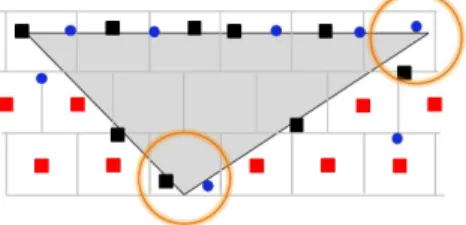
The neighborhood of a sensor node may change due to obstacles. Some neighboring nodes are no longer neighbors due to the presence of opaque obstacles. Then, the number of active nodes is not the same whether obstacles are opaque or transparent. We do not propose an additional condition to deal with opaque obstacles since OA-DVFA principle is still valid. Figures 1 and 2, show how OA-DVFA principle copes with both opaque and transparent obstacles. Small squares (red in the center of the cell, black otherwise) denote active sensor nodes, whereas redundant nodes in sleep state are denoted by small disks. In case of transparent obstacle (see Figure 1), only one sensor node per cell, the closest to the cell center, stay in active state, the others are considered as redundant nodes and should switch to sleep state. However, when the obstacle is opaque (see Figure 2), at least one node stay active in a cell. Since an opaque obstacle blocks the communication between nodes, two nodes can be in the same virtual cell but there are not neighbors. Then, both of them decide to stay in active state: see for instance the nodes within the orange circles.
Fig. 2: Opaque Obstacle. C. How to Run OA-DVFA
1) OA-DVFA for known obstacles: When obstacles are
known, the spreading time called Step1 Spread T ime, de-fined as the time needed to execute the node Spreading Step, can be estimated in advance. All nodes know the value of the spreading time, a parameter of OA-DVFA. They all enter Step 2 after this time, followed by Step 3. Notice that the Step1 Spread T ime is equal to 1500s for Topology 1 and 4000s for Topology 2. The execution of OA-DVFA is illustrated in Figure 3.
Fig. 3: Known obstacles: OA-DVFA.
2) OA-DVFA for unknown obstacles: When obstacles are
unknown, the spreading time cannot be estimated in advance. Sensor nodes should cooperate to decide when to stop the spreading step. This decision strongly depends on the coverage rate; as long as the coverage rate increases, node spreading should continue. The step 1 of the OA-DVFA algorithm is modified as depicted in Figure 4.
Since each node is able to determine the virtual cell to which it belongs, this information is used to estimate the coverage by computing the number of cells visited by sensor nodes. For this purpose, nodes exchange a bitmap message, where each node sets to 1 the bit corresponding to its cell. When a node receives the bitmap of its neighbors it updates its bitmap by making a logic OR between its bitmap and the bitmap received. The coverage is estimated by the number of 1 in the bitmap. However due to the presence of obstacles, all cells cannot be occupied by sensor nodes. We notice that if the number of visited cells in the bitmap increases, the coverage rate increases too. Hence nodes spreading should continue. Otherwise, the Spreading Step is ended.
To reduce the overhead, the exchange of bitmap mes-sage is limited. Initially, nodes spread without exchang-ing bitmap messages durexchang-ing a time Initial Spread T ime.
This time must be higher than or equal to the DiagonalLmax ∗
Hello P eriod to allow nodes to reach the corner opposite to the sink. In the performance evaluation of Section IV, we
get Initial Spread T ime ≥ 500∗
√ 2
5 ∗ 2.9 = 410s.
After this time, nodes continue to spread while exchanging bitmap messages during Bitmap Spread T ime. After this time, all nodes check whether the number of visited cells
re-mains constant. If yes, they end the Spreading step. Otherwise, they continue to spread during Spread T ime but without exchanging bitmap messages.
Fig. 4: Unknown obstacles: OA-DVFA. IV. PERFORMANCEEVALUATION
A. Simulation Parameters
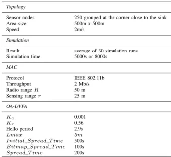
The parameters used in the simulations are defined in Table I. Notice that the optimal number of sensors needed to provide full coverage of the network area is 178 when the area does not contain any obstacle.
TABLE I: Simulation parameters
Topology
Sensor nodes 250 grouped at the corner close to the sink Area size 500m x 500m
Speed 2m/s Simulation
Result average of 30 simulation runs Simulation time 5000s or 8000s MAC Protocol IEEE 802.11b Throughput 2 Mb/s Radio range R 50 m Sensing range r 25 m OA-DVFA Ka 0.001 Kr 0.56 Hello period 2.9s Lmax 5m
Initial Spread T ime 500s Bitmap Spread T ime 100s Spread T ime 200s
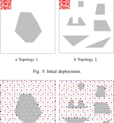
For this performance evaluation we consider an area of 500m ∗ 500m with obstacles whose surface occupy 20% of this area. We distinguish two topologies: Topology 1 (see Figure 5a) with only one obstacle and Topology 2 with 6 obstacles (see Figure 5b). Notice that both topologies have the same total surface of obstacles. These two topologies allow us to evaluate the impact of the number, shape and position of obstacles. All the simulation results are drawn with the 95% confidence interval.
B. Coverage rate
In this section, we evaluate the coverage rate. The coverage rate is computed as follows. The area considered is divided into
a Topology 1. b Topology 2.
Fig. 5: Intial deployment.
a Topology 1. b Topology 2.
Fig. 6: Final deployment.
squares of unit size. A unit square is considered covered if the center of this square is in the sensing range of at least one sensor node.
Figure 7 and Figure 8 illustrate the coverage rate as a function of time when all obstacles are known (see Figure 7) and all obstacles are unknown (see Figure 8). In each figure, the coverage rate is depicted for topologies 1 and 2. In both Figures, the curves depicting the coverage obtained for a given initial topology are identical in the two cases: all nodes are active or only those selected in step 3. We observe in Figure 7 that full coverage is reached in both topologies when all obstacles are known. As expected, Topology 2, the most complex topology, requires a longer time (i.e. 4000s) to reach a 100% coverage rate, whereas the deployment in Topology 1 is much faster, needing only 1000s. This highlights the impact of the number, shape and position of obstacles.
When we focus on unknown obstacles (in Figure 8), full coverage is reached with Topology 1. With Topology 2, OA-DVFA provides a coverage rate of 98%, which is a very good result for complex topology.
When obstacles are unknown, sensor nodes do not know the number of virtual cells that should be covered (i.e they do not know how many cells are occupied by obstacles). Since Topology 2 is complex, the stopping condition in the node spreading step of OA-DVFA may be true even if all cells have not yet been visited. OA-DVFA stops even if coverage is 98%. This can be explained by the following observation. At the beginning of the algorithm, the density of nodes is high and then the repulsive forces are high. Hence, the spreading of nodes is quick. Closer to the stability point, smaller are the
virtual forces and then the spreading of nodes becomes slow. In addition, the spreading of nodes can be slowed by the presence of obstacles causing a narrow lane in the area considered. To limit the distance traveled and hence the energy consumed by nodes, we prefer to stop sensor nodes prematurely rather than to move a longer time to gain 2% of coverage.
As a conclusion, OA-DVFA succeeds in providing a very good coverage rate, even when obstacles are discovered dynamically. As expected, to obtain a high coverage rate requires more time when obstacles are unknown.
0 20 40 60 80 100 0 1000 2000 3000 4000 5000 Coverage (%) Time (s)
OA-DVFA: coverage with all nodes (topology 1) OA-DVFA: coverage with all nodes (topology 2) OA-DVFA: coverage with only active nodes (topology 1) OA-DVFA: coverage with only active nodes (topology 2)
Fig. 7: Known obstacles: coverage as function of time.
0 20 40 60 80 100 0 1000 2000 3000 4000 5000 6000 7000 8000 Coverage (%) Time (s)
OA-DVFA: coverage with all nodes (topology 1) OA-DVFA: coverage with all nodes (topology 2) OA-DVFA: coverage with only active nodes (topology 1) OA-DVFA: coverage with only active nodes (topology 2)
Fig. 8: Unknown obstacles: coverage as function of time.
C. Distance traveled by nodes
We now focus on the distance traveled by nodes. We depict the accumulated distance traveled by all nodes during the deployment. We notice that in Figure 9 when obstacles are known, and in Figure 10 when obstacles are unknown, all nodes stop moving according to Step 2 of OA-DVFA. Hence the total distance traveled remains constant after this time. We conclude that OA-DVFA avoids node oscillations, a drawback inherent to virtual forces.
D. Active nodes
Since the area may contain unknown obstacles, the number of sensor nodes required cannot be computed in advance. Then, the number of sensor nodes initially present is higher than the required number.
0 50 100 150 200 250 300 350 400 450 0 1000 2000 3000 4000 5000 Distance (10 3m) Time (s) OA-DVFA (Topology 1) OA-DVFA (Topology 2)
Fig. 9: Known obstacles: total distance traveled by nodes as function of time. 0 50 100 150 200 250 300 350 400 0 1000 2000 3000 4000 5000 6000 7000 8000 Distance (10 3m) Time (s) OA-DVFA (Topology 1) OA-DVFA (Topology 2)
Fig. 10: Unknown obstacles: total distance traveled by nodes as function of time.
where only nodes needed to ensure full area coverage are active, the others switch to sleep state. Notice that as illustrated in Figure 7 and Figure 8, the coverage rate obtained by only active nodes (e.g. 151 active nodes in Topology 1 and 155 active nodes in Topology 2 of Figure 11) is the same as if all nodes (e.g. 250 nodes for both topologies of Figure 11) were active.
When obstacles are unknown, we get very close results as those with known obstacles, in terms of the number of active nodes as depicted in Figure 12. However, it may take more time.
Considering Step 2 and Step 3, we can conclude that OA-DVFA is an energy-efficient self-deployment algorithm.
V. CONCLUSION
In this paper, we propose a self-deployment algorithm, fully distributed, called OA-DVFA able to cope with unknown obstacles. OA-DVFA is based on virtual forces to ensure full area coverage and maintain network connectivity. OA-DVFA is designed to avoid the drawbacks inherent to virtual forces such as node oscillation and detection of the end of the algorithm. The performance evaluation, done by simulation, shows that OA-DVFA provides a very good coverage even when obstacles are unknown and the topology is complex. In OA-DVFA, sensor nodes are autonomous and able to detect the end of the deployment algorithm in a fully distributed way and then stop moving. 0 50 100 150 200 250 0 1000 2000 3000 4000 5000
Number of active nodes
Time (s)
OA-DVFA Topology 1 OA-DVFA Topology 2
Fig. 11: Known obstacles: number of active nodes.
0 50 100 150 200 250 0 1000 2000 3000 4000 5000 6000 7000 8000
Number of active nodes
Time (s)
OA-DVFA Toplogy 1 OA-DVFA Topology 2
Fig. 12: Unknown obstacles: number of active nodes. REFERENCES
[1] C.-Y. Chang, J.-P. Sheu, Y.-C. Chen, and S.-W. Chang, “An obstacle-free and power-efficient deployment algorithm for wireless sensor networks,” IEEE Transactions on Systems, Man and Cybernetics, Part A: Systems and Humans, vol. 39, no. 4, pp. 795–806, 2009.
[2] C.-Y. Chang, Y.-C. Chen, and H.-R. Chang, “Obstacle-resistant deploy-ment algorithms for wireless sensor networks,” IEEE Transactions on Vehicular Technology, vol. 58, no. 6, pp. 2925–2941, 2009.
[3] B. Sarazin and S. Rizvi, “A self-deployment obstacle avoidance (SOA) algorithm for mobile sensor networks,” International Journal of Com-puter Science and Security (IJCSS), vol. 4, no. 3, pp. 316–330, 2010. [4] X. Bai, S. Kumar, D. Xuan, Z. Yun, and T. H. Lai, “Deploying wireless
sensors to achieve both coverage and connectivity,” in Proceedings of the 7th ACM international symposium on Mobile ad hoc networking and computing, 2006, pp. 131–142.
[5] Y. Zou and K. Chakrabarty, “Sensor deployment and target localization based on virtual forces,” in IEEE INFOCOM, vol. 2, 2003, pp. 1293– 1303.
[6] K. Chakrabarty and S. Iyengar, “Sensor node deployment,” Scalable Infrastructure for Distributed Sensor Networks, Springer, pp. 19–55, 2005.
[7] G. Tan, S. A. Jarvis, and A.-M. Kermarrec, “Connectivity-guaranteed and obstacle-adaptive deployment schemes for mobile sensor networks,” IEEE Transactions on Mobile Computing, vol. 8, no. 6, pp. 836–848, 2009.
[8] K. Mougou, S. Mahfoudh, P. Minet, and A. Laouiti, “Redeployment of randomly deployed wireless mobile sensor nodes,” in Vehicular Technology Conference (VTC Fall), 2012 IEEE, 2012, pp. 1–5. [9] S. Mahfoudh, I. Khoufi, P. Minet, and A. Laouiti, “GDVFA: A
dis-tributed algorithm based on grid and virtual forces for the redeployment of WSNs,” in Wireless Communications and Networking Conference (WCNC), 2014 IEEE, 2014, pp. 3040–3045.