Walking Stability of a Variable Length Inverted Pendulum Controlled with Virtual Constraints

(1)

HAL Id: hal-02475100

https://hal.archives-ouvertes.fr/hal-02475100

Submitted on 11 Feb 2020

HAL is a multi-disciplinary open access

archive for the deposit and dissemination of

sci-entific research documents, whether they are

pub-lished or not. The documents may come from

teaching and research institutions in France or

abroad, or from public or private research centers.

L’archive ouverte pluridisciplinaire HAL, est

destinée au dépôt et à la diffusion de documents

scientifiques de niveau recherche, publiés ou non,

émanant des établissements d’enseignement et de

recherche français ou étrangers, des laboratoires

publics ou privés.

To cite this version:

Qiuyue Luo, Christine Chevallereau, Yannick Aoustin. Walking Stability of a Variable Length Inverted

Pendulum Controlled with Virtual Constraints. International Journal of Humanoid Robotics, World

Scientific Publishing, 2019, pp.1950040. �10.1142/S0219843619500403�. �hal-02475100�

(2)

Walking Stability of a Variable Length Inverted Pendulum Controlled with Virtual Constraints

Qiuyue Luo∗

Laboratoire des Sciences du Numérique de Nantes (LS2N), CNRS, Centrale Nantes, Université de Nantes, 1 rue de la Noë

Nantes, 44321, France qiuyue.luo@ls2n.fr Christine Chevallereau

Nantes, 44321, France christine.chevallereau@ls2n.fr

Yannick Aoustin

Nantes, 44321, France Yannick.Aoustin@univ-nantes.fr

Received Day Month Year Revised Day Month Year Accepted Day Month Year

Bipedal walking is a complex phenomenon that is not fully understood. Simplified mod-els make it easier to highlight important features. Here the variable length inverted pendulum (VLIP) model is used, which has the particularity of taking into account the vertical oscillations of the center of mass (CoM). When the desired walking gait is de-fined as virtual constraints i.e. as functions of a phasing variable and not on time, for the evolution of the swing foot and the vertical oscillation of the CoM, the walk will asymptotically converge to the periodic motion under disturbance with proper choice of the virtual constraints, thus a self-stabilization is obtained. It is shown that the vertical CoM oscillation, positions of the swing foot and the choice of the switching condition play crucial roles in stability. Moreover, a PI controller of the CoM velocity along the sagittal axis is also proposed such that the walking speed of the robot can converge to another periodic motion with a different walking speed. In this way, a natural walking gait is illustrated as well as the possibility of velocity adaptation as observed in human walking.

Keywords: Variable length inverted pendulum (VLIP); Hybrid model; Virtual con-straints; Self-stabilization; Biped.

∗_{Corresponding author.}

(3)

1. Introduction

Humanoid robots are very complex systems with high degrees-of-freedom (DoF). In order to study the essential factor of the walking gait, the simplified models are usually used. One of the mostly used simplified models is the 3D linear inverted

pendulum (LIP) model proposed by S. Kajita1_{, which regards the robot as a}

con-centrated mass with a zero vertical acceleration. The 3D LIP model is interesting because an analytical expression to define the center of mass (CoM) evolution exists and its dynamics in sagittal and frontal planes are decoupled.

However, in human walk, the height of the CoM is not constant, and the

ver-tical oscillation of the CoM must be considered2;3. Authors in Ref.2 observed that

during walking the maximum vertical displacement increases from 0.013 ± 0.001 m

(mean±S.E.M.) for a walking speed 0.5 ms−1 _{to 0.031 ± 0.007 m for a walking}

speed 2.5 ms−1. Several approaches have been proposed to extend the LIP to have

a more human-like behavior. Omran et al.4_{investigated the effect of vertical motion}

of the CoM during humanoid walking. Numerical tests show a consequent reduc-tion of the robot torque solicitareduc-tion when the CoM oscillates vertically. Garofalo et

al.5 mapped the simple dynamics of the bipedal spring loaded inverted pendulum

(SLIP) model to multi-body robots to obtain a desired behavior for the CoM, yet an upper level controller is necessary to deal with the stabilization of the SLIP model.

Harada et al.6_{captured the walking motion of a human, and applied the obtained}

information on real humanoid robot. The variable length inverted pendulum (VLIP) model is used in this paper. Contrary to the SLIP model, a rigid model of the leg is used and the vertical oscillations of the CoM results from the control strategy. At the end of each step, the vertical velocity of the CoM points downwards, and the vertical movement of the CoM is a polynomial based on boundary conditions. It has been proven that the vertical oscillations induce a self-stabilization of the walk for

specific virtual constraints7_{. The current paper extends these preliminary results}

into a more systematic study of the virtual constraint by extending the results of

self-synchronization obtained with a LIP model8.

For a robot with feet, the necessary and sufficient condition of stable locomotion is to have the Zero-Moment-Point (ZMP) within the support polygon at all stages

of the locomotion gait9;10;11_{. For robots with point feet, this condition means at}

at each time, the robot is in dynamical equilibrium. In single support phase, the dynamic equilibrium defines the angular acceleration around the point of contact, and the concept of ZMP is not directly applicable to such systems. Absence of active

actuation at the ankles makes these systems under-actuated. The Poincar´e return

map12;13_{is the appropriate mathematical tool for analyzing the stability of periodic}

orbits for under-actuated systems. In this context, the stability is the convergence toward an orbit or periodic motion.

In order to avoid falling down, when and where to place the swing foot is essen-tially important. For a robot that only follows a pre-defined walking gait, a small disturbance on the ground or mass distribution may change the original walking

(4)

direction of the robot, or even cause the robot to lose balance. In Ref.14_{and Ref.}15_,

a constant period is assumed, and a preview control over several steps is considered

for gait planning. Takenaka et al.16 _{proposed an approach based on the}

diver-gent component of motion (DCM) to generate walking patterns with good stability

properties. Hopkins et al.17 proposed a time varying DCM for better tracking of

the vertical component of the DCM during walking on uneven grounds. Englsberger et al., by using the same property of decomposition into an intuitive way as two cascaded first-order systems, derived a capture point controller (CP), which exploits

the natural dynamics of the LIP in order to get a gait pattern generator18_{. This}

result was extended to three dimension in Ref.19_{. Approaches presented in Ref.}20

and Ref.21_{modify both the step timing and step length on-line to control the}

walk-ing speed under small or medium disturbances. However, these approaches can be only applied for the LIP model, and the stable walking is based on the prediction of future states of the CoM and foot locations.

For under-actuated robots, virtual constraints are functional relations among the

system’s states that are imposed via a feedback controller12_{. In order to synchronize}

the evolution of the various links, an internal phasing variable is used such as the

position of robot’s hip along the sagittal axis22_{. Griffin and Grizzle}23 _{introduced a}

class of virtual nonholonomic constraints that depend on velocity through (general-ized) angular momentum. Including angular momentum in the virtual constraints allows foot placement control to be designed on the basis of the full dynamic model of the biped. This method leads to a new class of control laws that are robust to a variety of common gait disturbances. Authors plane to extend this method to a 3D walking.

The objective of this paper is to find some physical conditions that lead to self-stabilization based on a simplified model with vertical CoM oscillation. A switching surface is proposed that when the robot’s CoM crosses the surface, the stance foot is switched. By doing this, the step timing is not explicitly but implicitly adapted under disturbances. To make sure that the swing foot touches the ground at the same time when the CoM crosses the switching surface, the trajectory of the swing foot is defined as a function of a phasing variable based on the feedback of the robot’s internal states instead of time. How the features of the switching surface and the vertical motion of the CoM affect the stability of the system has been analyzed.

As an extension of our previous work8_{, this paper proves that for a VLIP model,}

self-stabilization can be obtained when the switching condition is based on a linear combination of the CoM positions along the sagittal and frontal axes. Moreover, it is proved that when the CoM velocity feedback in the sagittal plane is taken into account, the system is able to converge asymptotically to a new periodic motion without the complex procedure of finding a periodic motion.

The paper is structured as follows. In Section 2, the hybrid model of the VLIP is detailed. In Section 3, the virtual constraint and the phasing variable are intro-duced. In Section 4, the periodic motion of VLIP is introintro-duced. In Section 5, the

(5)

stability of the VLIP model with the proposed switching conditions that leads to self-stabilization of the walking gait is analyzed. Simulations illustrate the property of self-stabilization. Section 6 shows how a feedback on walking velocity can be used to adapt the periodic motion to a desired walking speed. Finally, several concluding remarks and perspectives are discussed in Section 7.

2. Modeling

The gait is composed of two phases: single support phase and double support phase. During the double support phase, the following hypotheses are chosen: 1) The dou-ble support phase is instantaneous; 2) The contact between the swing foot and the

ground does not modify the velocity of the CoM24.

2.1. Variable Length Inverted Pendulum (VLIP) Model

During the single support phase, the VLIP model is used. Compared with LIP model, the VLIP model is closer to the real human walking behavior, because the height of the CoM is not constant during walking.

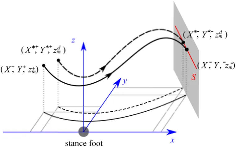
Fig. 1: The VLIP model.

The VLIP model consists of two massless legs with variable length and a concen-trated mass at the hip, as shown in figure 1. The stance leg is free to rotate about the axes x and y at the ground. The length of each leg can be modified through actuation, allowing a desired vertical motion of the pendulum to be obtained. We also assume that the actuation of the swing leg allows a controlled displacement of the swing leg end via hip and knee actuators.

The configuration of the robot is defined via the position of the concentrated

mass (xm, ym, zm) and the position of the swing foot (xs, ys, zs) with respect to a

(6)

y are denoted by σx and σy. In order to explore simultaneously the existence and

stability of periodic orbits for robots with any step length and width, a

dimen-sionless dynamic model is used7_{. The normalized scaling factors applied along x}

and y axes depend on desired step length S, desired step width D, and the robot

mass m. Thus, a new set of variables is defined: (X, Y, zm, Xs, Ys, zs, σX, σY) =

(xm S , ym D, zm, xs S, ys D, zs, σx mD, σy mS).

The variables (zm, Xs, Ys, zs) are chosen to be the controlled variables

deter-mined by virtual constraints as functions of the phasing variable Φ(X, Y ), where

X and Y are defined as free variables or uncontrolled variables qf = (X, Y ). The

definition of the phasing variable will be discussed in detail in Section 3.2. The height of the CoM and its velocity can be expressed as:

zm= f (Φ) ˙ zm= ∂f (Φ) ∂Φ ( ∂Φ ∂X ˙ X + ∂Φ ∂Y ˙ Y ) = ∂f ∂X ˙ X + ∂f ∂Y ˙ Y (1)

Since the legs are massless, the motion of the swing leg does not affect the dynamic model. The moment balance equation of the pendulum around the rotation axes x and y, with the normalized variable, directly yields the dynamic equation:

(

˙σX = −gY

˙σY = gX

(2)

For the VLIP, the angular momentum is: (σX = ˙zmY − zmY˙

σY = − ˙zmX + zmX˙

(3)

Assuming that the control law allows that the vertical motion of the CoM is

perfectly tracked, Eq. (1) can be used to rewrite the zero dynamics12 _{as :}

     ˙ qf = M_XY−1 · [σX; σY]> ˙σX = −gY ˙σY = gX (4) where MXY = " ∂f ∂XY ∂f ∂YY − f f −_∂Y∂fY −∂f ∂YX # (5)

2.2. Transition between steps

Due to the hypothesis of massless legs, the contact between the swing foot and the ground does not affect the velocity of the CoM, and the velocity of CoM is conserved at each transition of stance leg. Since the reference frame is always attached to the stance foot and the y axis is directed toward the CoM, the sign of the velocity along

(7)

y axis will be changed from positive to negative, i.e. ˙ X_k+1+ = ˙X_k−, ˙ Y_k+1+ = − ˙Y_k−, ˙ z+_m,k+1= ˙z_m,k− (6)

The state before the transition, i.e. at the end of a step, is expressed by

super-script− and that after the transition, i.e. at the beginning of a step, is expressed

by +_{. The variables corresponding to the step k, are denoted with index k, while}

those of the next step are denoted with k + 1.

After transition, the swing foot placement becomes the new stance foot place-ment. Thus the CoM position after transition along x axis equals to the CoM posi-tion before transiposi-tion minus the swing foot posiposi-tion. Similar result can be obtained for the CoM position along y axis:

X_k+1+ = X_k−− X_s,k−

Y_k+1+ = −Y_k−+ Y_s,k− (7)

Knowing the final state of the single support phase, the transition model (6) and (7) determines the initial state of the ensuing single support phase.

2.3. Hybrid model.

The transition occurs when the height of the swing foot zs is zero. A switching

manifold is defined below:

S := {x|zs= 0, ˙zs< 0} (8)

where x := [X, Y, zm, Xs, Ys, zs, ˙X, ˙Y , ˙zm, ˙Xs, ˙Ys, ˙zs]> is the state of the robot. The

transition model (6) and (7) can be rewritten as:

x+= ∆(x−) (9)

where ∆ indicates the transition map. Thus the combination of the dynamic equa-tions and the transition model (9) forms the single-phase hybrid dynamical system:

Σ : (

˙x = f (x) + g(x)u, x−∈/ S

x+= ∆(x−), x−∈S (10)

where u is the control law that allows us to track the reference trajectory of the swing foot and vertical motion of the CoM.

3. Virtual Constraints

A normalized variable Φ monotonically increasing from 0 to 1 during one step, named phasing variable is defined to describe the desired trajectories of the con-trolled variables. The trajectories of the swing foot and the vertical oscillation

of CoM are defined as a function of Φ: Xs = Xs(Φ), Ys = Ys(Φ), zs = zs(Φ),

(8)

the horizontal evolution determines foot locations. The advantage of introducing virtual constraints based on a phasing variable is that this method can be extended to a complete model of robots by using the phasing variable to coordinate all the joint motions of the robot.

3.1. Switching manifold

In paper8_{, it has been proven that when the transition of stance foot is based on}

time, the state of the robot will not converge to the fixed value when there exists an initial perturbation. Instead of time, the phasing variable based on the CoM

position X and Y proposed in paper8 _{is used here.}

The vertical trajectory of the swing foot is defined as a function of Φ(X, Y ). The transition happens when the swing foot touches the ground, which defines a relationship between the two variables X and Y . An infinite number of CoM positions satisfy it. This set of positions are grouped in the switching configuration manifold defined by:

S = {(X, Y )|zs(Φ) = 0}. (11)

The phasing variable is chosen such that the robot switches its stance leg when the CoM crosses the switching manifold:

S = {(X, Y )|(X − X∗−) + C(Y − Y∗−) = 0}. (12)

The switching manifold S is defined as a vertical surface parameterized by C, represented by the gray surface in figure 2. Many other sets of positions can be considered but since stability studied here is a local property, a flat surface is a convenient choice. The choice of S directly affects the final CoM position for step k.

3.2. Phasing Variable

As introduced in paper8, the phasing variable Φ is defined as a function of X and

Y with six parameters:

Φ = aX + bY + cXY + dX2+ eY2+ f (13)

and the phasing variable must vary from 0 to 1 for a step and be monotonic. Since

the phasing variable must be zero at the beginning of a step, Φ(X+_{, Y}+_{) = 0,}

where X+ and Y+ are known from Eq. (7). Besides, in order to make the

switch-ing manifold (11) and (12) equivalent, the phasswitch-ing variable at the end of a step

Φ(X−, Y−) = 1, for any X−= X∗−− Cδ and Y−_{= Y}∗−_{+ δ, where δ is the CoM}

position error along y axis at the end of a step. Since all the above constraints must be satisfied for an arbitrary value of δ, three more equations can be obtained and

(9)

x y z S stance foot - -( , , )X Y zm - -( , , )X Y zm -( , , )X Y zm ( , , )X Y zm + + + + + d d

Fig. 2: The step finishes when the CoM crosses the switching manifold, which is represented by the gray surface. The curved dashed line is the periodic motion, and the curved solid line the CoM motion under an initial perturbation.

we have:            aX++ bY++ cX+Y++ d(X+)2+ e(Y+)2+ f = 0 aX∗−+bY∗−+cX∗−Y∗−+d(X∗−)2+e(Y∗−)2+f = 1 −cC + dC2_{+ e = 0}

−aC +b−cCY∗−_+cX∗−_−2dCX∗−_+2eY∗−_{= 0.}

(14)

There are six variables {a, b, c, d, e, f } while the number of equations is only four, thus parameters a, b, e, and f can be obtained as functions of c and d. The values of c and d can be chosen based on some optimization standards. Here, the objective function is chosen to minimize the difference between Φ(t) and t to insure the monotony of Φ. That is:

J = Σ(Φ(t)i− ti)2 (15)

The matlab function fmincon is used off-line when virtual constraint are de-R

signed.

3.3. The Vertical Motion of the swing foot

An intermediate value of the phasing variable 0 < Φm< 1 is defined, so that when

Φ = Φm, hz = max

0<Φ<1{zs}. For the vertical motion of swing foot, the boundary

conditions are:

zs(0) = 0, zs(Φm) = hz, zs(1) = 0,

˙

zs(0) = 0, z˙s(Φm) = 0, z˙s(1) = vz,

(10)

where hz is the desired height of the swing foot when Φ = Φm, and vz< 0 denotes

the desired downward velocity of the swing foot at the end of a step. In this paper,

zs(Φ) is defined as a cubic spline.

3.4. The Horizontal Motion of the swing foot

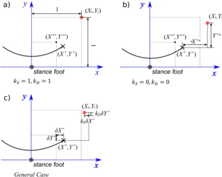
The position where to land the swing foot must be chosen cautiously. In order to analyze several cases, the swing foot positions at the end of step k is expressed in a generalized form: X_s,k− = (1 − kS)(Xk−− X ∗+_{) + k} SS Y_s,k− = (1 − kD)(Yk−+ Y∗+) + kDD (17)

where 0 ≤ kS ≤ 1 and 0 ≤ kD≤ 1. How the values of kS and kD affect the swing

Fig. 3: Influence of kS and kD on the foot locations. a) Step length and width are

fixed; b) The initial CoM position error is nullified; c) The general case. The black and the red dots represent respectively the stance feet during the current and the next steps. The curved line represents the CoM trajectory, and the cross the CoM position at the end of the current step.

foot positions is illustrated in figure 3. The case kS = kD = 0 allows to nullify the

(11)

0, δY_k+1+ = Y_k+1+ − Y∗+_{= 0. The case k}

S= kD= 1 corresponds to fixed step length

and width.

The boundary conditions for the motion of the swing foot along x direction

Xs(Φ) are:

Xs(0) =Xs,k+ , X˙s(0) = 0,

Xs(1) =X_s,k− , X˙s(1) = 0,

(18)

where X_s,k+ is the swing foot position at the beginning of step k, and it can be

known according to the information of the previous step. The velocity at the end of the step is chosen null to have a vertical motion of the swing foot and to increase robustness with respect ground disturbance.

The same constraints are imposed on the motion along y direction Ys(Φ). With

these boundary conditions, the trajectories along x and y directions can be defined as third order polynomial functions of Φ.

3.5. Vertical Oscillation of the CoM

It has been proven in Ref.7that the vertical oscillation of the CoM can

asymptoti-cally stabilize a periodic walking gait. A polynomial that keeps the motion of CoM continuous is used considering the following constraints:

zm(0) = zm+; zm(1) = zmd;

˙

zm(0) = ˙zm+; ˙zm(1) = ˙zdm

(19) The oscillations chosen are such that the final velocity for each step is negative i.e. ˙zd

m< 0.

4. Periodic gait of VLIP

For a VLIP, the change of support is characterized by a change of the point where

the angular momentum is calculated, thus we have7:

(

σ_X+ = σ−_X− D ˙zm−

σ_Y+= −σ−_Y + D ˙z_m− (20)

As the vertical velocity of the CoM right before the change of support is negative,

it implies that the angular momenta σX and σY decrease at the change of support.

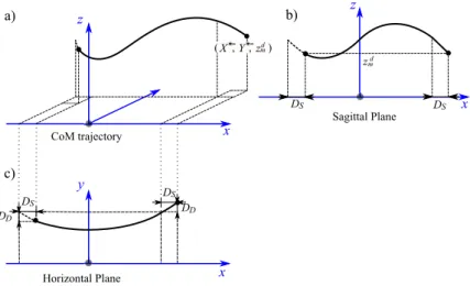
In order to obtain a periodic motion, the angular momenta must therefore increase during the stance phase, and thus it is necessary to slightly shift the relative position of the support leg and the CoM. The position of the CoM at the beginning of the

step is then written as X+ = −1/2 + DS, Y+ = 1/2 − DD and at the end of the

step X−= 1/2 + DS, Y− = 1/2 + DD with DS =X +_+X− 2 ≥ 0 and DD= Y −_−Y+ 2 , as shown in figure 4.

Since the model of walking is a hybrid model as shown in Section 2.3, a classical

(12)

CoM trajectory x x x z z y DD Sagittal Plane Horizontal Plane a) c) b) DS DS DD DS DS zmd - -( , , )X Y zmd

Fig. 4: The CoM trajectory of a periodic motion, and its projections in sagittal and horizontal planes.

map. In this study, we assume that a perfect tracking of the controlled variables

is obtained, and the Poincar´e section is defined by Eq. (12). In this context, since

virtual constraints expressed as functions of Φ(X, Y ) are used,the state of the robot

in the Poincar´e section is reduced to [X−; Y−; ˙X−; ˙Y−] and the Poincar´e return

map can be written: .

[X_k+1− , Y_k+1− , ˙X_k+1− , ˙Y_k+1− ] = f (X_k−, Y_k−, ˙X_k−, ˙Y_k−) (21)

The periodic motion is characterized by the fixed point of the Poincar´e return

map and satisfy :

[X_k−, Y_k−, ˙X_k−, ˙Y_k−] − f (X_k−, Y_k−, ˙X_k−, ˙Y_k−) = 0 (22)

The elements DS = X_k−− 1/2, DD = Y_k− − 1/2, ˙X_k−, ˙Y_k− are calculated by a

given initial guess and matlab function f solve with Eq. (22). As this optimizationR

technique is applied for normalized parameters, the corresponding periodic steps for any step length and step width can be deduced.

5. The stability of control strategy applied to the VLIP model

The stability of the walking gait based on the virtual constraints defined in Section

3 is now analyzed via the stability of the Poincar´e return map. A stable walking

is obtained when all the norms of the eigenvalues of the Jacobian of the poincar´e

return map are strictly less than 1.

Since X− and Y− are coupled via the switching manifold, the Jacobian matrix

of the Poincar´e return map at the fixed point and its eigenvalues are calculated

(13)

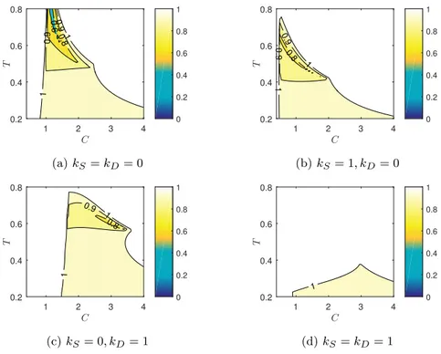
5.1. Influence of kS and kD on the stability

The values of kS and kD determine the landing position of the swing foot, and

consequently the initial CoM position for the next step. From the study with the

LIP model8_{, we have obversed that theses parameters are crucial for the stability}

of walking, thus the effect of these parameters is now considered in the case of

VLIP model. Cases for different values of kS and kD are studied here. The other

parameters are: ˙zd

m = −0.1m/s, zmd = 0.7m. The value ˙zdm = −0.1m/s has been

chosen according to the human vertical oscillations of the CoM. It has to be noted that in our study the double support phase is considered as an instantaneous phase, while it is not instantaneous in human walk. This assumption of instantaneous phase is made to simplify the study and due to the fact that it increases the difficulty to have stable walking as the stability margin can be improved using double support

phase25_{. The evaluation of a pertinent choice of ˙}_zd

m to mimic human like gait is

not obvious since it varies with the placement of the instantaneous double support

phase in the gait, thus we consider that a value 0 ≤ ˙z_md ≤ −0.2m/s is convenient.

0.6 0.8 0.9 0.9 1 1 1 2 3 4 C 0.2 0.4 0.6 0.8 T 0 0.2 0.4 0.6 0.8 1 (a) kS = kD= 0 0.8 0.9 0.9 1 1 1 2 3 4 C 0.2 0.4 0.6 0.8 T 0 0.2 0.4 0.6 0.8 1 (b) kS = 1, kD= 0 0.8 0.9 1 1 1 2 3 4 C 0.2 0.4 0.6 0.8 T 0 0.2 0.4 0.6 0.8 1 (c) kS= 0, kD= 1 1 1 2 3 4 C 0.2 0.4 0.6 0.8 T 0 0.2 0.4 0.6 0.8 1 (d) kS= kD= 1

Fig. 5: Influence of kS and kD on the eigenvalues. Contrary to the white areas, the

colored areas indicate self-stabilization condition.

(14)

initial CoM error in position is smaller, larger stability region can be obtained. When

kS = 1, the proper value of T for stability is too small, only very fast step can be

achieved with stability. Thus kS = 0 appears to be a good choice for stable walking.

The choice of kD≤ 1 has a smaller effect on the possibility to have stable walk with

sufficient step duration. In the following we will consider the case kS = 0, kD = 0,

that corresponds to placing the foot in order to nullify the initial error on the CoM position in horizontal plane for the next step. In presence of perturbation, this

choice will induce some deviation in the lateral axis since kD = 0 will prevent the

robot to have a strict straight line motion7. In order to be able to avoid this lateral

motion, the specific case kS = 0, kD= 1 is also considered for the following sections

where the influence of the choice of ˙zdmis considered.

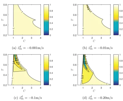
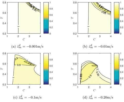
5.2. Influence of C, T and ˙z_md on the stability

In order to study the influence of C, T and ˙zmd on the eigenvalues, the values of zmd

is taken as constant: zd

m= 0.7m. The results of the eigenvalues as a function of C

and T for ˙zdm = −0.001m/s, ˙zmd = −0.01m/s, ˙zmd = −0.1m/s and ˙zmd = −0.2m/s

are calculated for the cases kS = 0, kD= 0 (shown in figure 6) and kS = 0, kD= 1

(shown in figure 7).

It can be seen from figures 6 and 7 that the bigger ˙zd

mis, the smaller the

eigen-value is, which means faster convergence. For the case kS = 0, kD= 1, along with

the increase of ˙zmd, the proper values of T and C that satisfy the stability

condi-tion will decrease. When kS = 0, kD= 0, the eigenvalues are smaller than the case

kS = 0, kD = 1, but the safety margin is smaller when T is big. In order to obtain

self-stabilization, the value of ˙zd

mmust be chosen cautiously according to the desired

step timing or walking velocity. 5.3. Simulations

In order to test the robustness and self-stabilization of the walking algorithm,

simu-lations for kS = 0, kD= 0 and kS= 0, kD= 1 are made. The step length and width

S = 0.3m, D = 0.15m are taken, while the desired height and vertical velocity of the

CoM at the end of a step for a periodic motion are: zd

m= 0.7m and ˙zmd = −0.1m/s

respectively. When T = 0.6s, according to the results shown in figures 6c and 7c,

C = 1.2 and C = 2.5 are proper values for obtaining self-stabilization when kS= 0,

kD = 0 and kS = 0, kD= 1 respectively. When the key parameters describing the

walking are chosen, the virtual constraints can be defined (see Section 3) and the periodic motion can be calculated (see Section 4).

In the simulations, we integrate a starting and stopping configuration where the robot is assumed to be in double support and to have a rest configuration. For the first step, the CoM of VLIP starts from a position close to the future stance foot with a zero velocity, and for the last step, the CoM stops at a position close to the previous stance foot. As for the first and the last steps, the motion of the CoM is far from the periodic motion, the phasing variable is chosen to be a function of

(15)

1 1 1 2 3 4 C 0.2 0.4 0.6 0.8 T 0 0.2 0.4 0.6 0.8 1 (a) ˙zmd = −0.001m/s 0.9 1 1 1 2 3 4 C 0.2 0.4 0.6 0.8 T 0 0.2 0.4 0.6 0.8 1 (b) ˙zmd = −0.01m/s 0.6 0.8 0.9 0.9 1 1 1 2 3 4 C 0.2 0.4 0.6 0.8 T 0 0.2 0.4 0.6 0.8 1 (c) ˙zdm= −0.1m/s 0.6 0.7 0.9 0.9 1 1 1 1 2 3 4 C 0.2 0.4 0.6 0.8 T 0 0.2 0.4 0.6 0.8 1 (d) ˙zmd = −0.20m/s

Fig. 6: Maximal norm of eigenvalues for different ˙zd

mwhen kS = 0, kD= 0. Contrary

to the white areas, the colored areas indicate self-stabilization condition.

time. In order to obtain a CoM velocity of the VLIP in horizontal plane close to the periodic one at the end of the first step, the LIP model is used to estimate the

initial CoM position for the first step24_:

x0= ˙ x∗ sinh(ωT )ω; y0= ˙ y∗ sinh(ωT )ω (23)

where ω =pg/zmcharacterizes the LIP. With the same initial CoM position, at the

end of the first step, the CoM of the VLIP will end up with smaller velocity along x axis than LIP. In order to increase the safety margin, the maximum CoM height

of the VLIP is taken when calculating x0 and y0. At the last step, an optimization

(16)

0.9 0.95 0.95 1 1 1 2 3 4 C 0.2 0.4 0.6 0.8 T 0 0.2 0.4 0.6 0.8 1 (a) ˙zmd = −0.001m/s 0.9 0.9 0.95 0.95 1 1 1 2 3 4 C 0.2 0.4 0.6 0.8 T 0 0.2 0.4 0.6 0.8 1 (b) ˙zmd = −0.01m/s 0.8 0.9 0.9 ₁ 1 1 2 3 4 C 0.2 0.4 0.6 0.8 T 0 0.2 0.4 0.6 0.8 1 (c) ˙zmd = −0.1m/s 0.9 0.9 0.95 0.95 1 1 1 2 3 4 C 0.2 0.4 0.6 0.8 T 0 0.2 0.4 0.6 0.8 1 (d) ˙zmd = −0.20m/s

mwhen kS = 0, kD= 1. Contrary

to the white areas, the colored areas indicate self-stabilization condition.

0 1 2 3 4 5 6 7 8 -0.02 0 0.02 0.04 0.06 0.08 0.1 0.12 0.14 0.16

Fig. 8: The projection of the VLIP motion in horizontal plane for 25 steps when

kS = 0, kD = 0. The black curves represent the CoM evolution, the blue circles

represent the stance foot placements, and the blue lines represent the swiching manifold.

(17)

0 5 10 15 20 25 step -0.1 0 0.1 0.2 0.3 x [m ]

the real value the desired value

0 5 10 15 20 25 step 0 0.02 0.04 0.06 0.08 y [m ]

0 5 10 15 20 25 step 0 0.2 0.4 0.6 0.8 ˙x[ m /s ]

0 5 10 15 20 25 step -0.1 0 0.1 0.2 0.3 ˙y[ m/s

] the real value

the desired value

Fig. 9: CoM position and velocity evolutions for 25 steps when kS = 0, kD= 0 in

the local reference frame.

As shown in figure 8, for the case when kS = 0, kD = 0, the CoM of the

pendulum starts from a position close to the stance foot with a zero velocity. A change of the landing position of the swing foot along y axis can be observed. This is due to the fact that the landing position strategy consists to nullify the initial CoM position error. From figure 9, it can be seen that after the first step, the system has a state different from that of the periodic motion, converges asymptotically to the periodic motion for the following steps, and stops close to the stance foot with a

zero velocity during the last step. For the case when kS = 0, kD= 1, similar results

are obtained, as shown in figures 10 and 11. In this case, except for the first and the last steps which use a different landing strategy, the landing positions of the swing foot stay in a straight line i.e. the step width is constant. Faster convergence can

be observed for the case kS = 0, kD= 0, which corresponds to the results shown in

figure 5.

6. Change of the walking velocity

Due to the self-stabilization property of the control approach based on virtual constraints, different virtual constraints correspond to different walking velocities. When the humanoid has to adapt its walking velocity, the virtual constraints have to be changed. This can be done for example by inclining forward the torso to

in-crease the walking velocity12. In this section we explore the possibility to be able to

adapt the walking velocity without recomputing new virtual constraints but only based on a feedback on the current walking speed. Different from the method

(18)

pro-0 2 4 6 8 10 12 -0.02 0 0.02 0.04 0.06 0.08 0.1 0.12 0.14

posed by Apostolopoulos et el. in Ref.26, the complex procedure of calculating the

new periodic motion is unnecessary in this work.

It has been proven in Ref.8_{that the feedback of the CoM velocity along sagittal}

axis can provide self-stabilization for a LIP model. How this feedback affects the stability of a VLIP model is discussed here. By introducing the feedback of the walking speed, a new switching manifold was proposed:

Sv= {(X, Y )|(X − X∗−− l) + C(Y − Y∗−) = 0}. (24)

As shown in figure 12, the new switching manifold Svis a surface with an offset

l from the switching manifold proposed in Section 3.1 along x axis. The offset is

defined as l = kv( ˙X∗+− ˙Xk+), where ˙X

+

k is the CoM velocity along x axis at

the beginning of step k. It allows to adjust the position of the switching manifold

according to the velocity feedback of the CoM for each step. kv is a parameter that

must be chosen carefully to satisfy the stability condition.

6.1. Influence of C and kv on the stability

Here, T = 0.6s is taken and eigenvalues are calculated as functions of C and kv

for ˙zmd = 0m/s and ˙zmd = −0.1m/s. The results of two cases kS = 0, kD = 0 and

kS = 0, kD= 1 are shown in figures 13 and 14 respectively.

(19)

0 10 20 30 40 step -0.1 0 0.1 0.2 x [m ]

0 10 20 30 40 step 0 0.02 0.04 0.06 0.08 y [m ]

0 10 20 30 40 step 0 0.5 1 ˙x[ m /s ]

0 10 20 30 40 step 0 0.1 0.2 0.3 ˙y[ m/s ]

Fig. 11: CoM position and velocity evolutions for 40 steps when kS = 0, kD = 1 in

x y z Sv S l - -( , , )X Y zm -( , , )X Y z+ m + _d ( , , )X Y zm + + +

Fig. 12: The step finishes when the CoM crosses the switching manifold, which is represented by the darker gray surface. The curved dashed line is the periodic motion, and the curved solid line is the CoM motion under an initial position perturbation.

the case ˙zmd = 0m/s), stability is obtained only for positive value of kv. Contrary to

this, it can been seen from figures 13b and 14b that when kv = 0, the eigenvalues

(20)

0.4 0.6 0.8 0.8 1 1 1 0.5 1 1.5 2 2.5 3 C 0 0.1 0.2 0.3 kv 0 0.2 0.4 0.6 0.8 1 (a) ˙zmd = 0m/s 0.40.6 0.8 0.8 1 1 0.5 1 1.5 2 2.5 3 C 0 0.1 0.2 0.3 kv 0 0.2 0.4 0.6 0.8 1 (b) ˙zdm= −0.1m/s

m as a function of C and kv when kS = 0, kD= 0. 0.8 0.8 0.9 0.9 1 1 1 1 2 3 4 C 0 0.05 0.1 kv 0 0.2 0.4 0.6 0.8 1 (a) ˙zmd = 0m/s 0.9 0.9 0.95 0.95 1 1 1 1 2 3 4 C 0 0.05 0.1 kv 0 0.2 0.4 0.6 0.8 1 (b) ˙zdm= −0.1m/s

m as a function of C and kv

when kS = 0, kD= 1.

to guarantee convergence to a periodic gait. From figure 13b, it can be seen that a

positive value of kv helps to decrease the amplitude of the eigenvalue when kS =

0, kD = 0, while the effect is not so obvious when kS = 0, kD = 1 as shown in

figure 14b. However, for both cases, a feedback on the CoM velocity to define the switching manifold is useful if a specific walking velocity is desired.

6.2. Simulations

This section illustrates the change of switching manifold to control the walking velocity of the robot along the axis x. The same virtual constraints are used for all

the simulations with desired velocities ˙X∗+ and ˙X∗++ ∆ ˙X.

Since the periodic motions for different velocities correspond to different X∗−

(21)

of the switching manifold (24) does not allow to reach the desired velocity. In order to compensate the static error, an integration term of the velocity error is

added into the offset l, which gives l = kv( ˙X∗+− ˙Xk+) + kI

k

P

i=1

( ˙X_i∗+− ˙X_i+). The

introduction of kv and kI allows the CoM to converge to a new periodic motion

without defining explicitly the new periodic gait. While the desired CoM velocity along x axis increases (or decreases), its velocity along y axis will decrease (or increase) correspondingly.

The same parameters as in Section 5.3 are taken: S = 0.3m, D = 0.15m, T = 0.6s, zd

m = 0.7m and ˙zdm = −0.1m/s. The values of kv and C are chosen to be

kv= 0.08, C = 1.1 for the case kS = 0, kD= 0 and kv= 0.03, C = 2.5 for the case

kS = 0, kD= 1 respectively based the results from figures 13b and 14b. At the 10th

step, the desired CoM velocity along x axis ˙x∗+_m is increased by 0.2m/s.

0 2 4 6 8 10 12 x[m] -0.05 0 0.05 0.1 0.15 0.2 y [m ]

It can be seen from figures 15 and 17 that along with the increase of walking

speed, the amplitude of the lateral CoM oscillations is reduced. For the case kS = 0,

kD = 0 (shown in figure 15), a large change of position along y axis can be also

observed, while for the case kS = 0, kD = 1 (shown in figure 17), the robot keeps

walking along a straight line despite of the change of speed. From figures 16 and 18,

(22)

0 10 20 30 40 step -0.1 0 0.1 0.2 0.3 x [m ]

the real value

0 10 20 30 40 step 0 0.05 0.1 y [m ]

the real value

0 10 20 30 40 step 0 0.5 1 ˙x[ m /s ]

0 10 20 30 40 step -0.1 0 0.1 0.2 0.3 ˙y[ m/s ]

the real value

0 5 10 15 x[m] -0.02 0 0.02 0.04 0.06 0.08 0.1 0.12 0.14 y [m ]

(23)

0 10 20 30 40 50 step -0.1 0 0.1 0.2 x [m

] the real value

0 10 20 30 40 50 step 0 0.05 0.1 y [m ]

the real value

0 10 20 30 40 50 step 0 0.5 1 ˙x[ m /s ]

0 10 20 30 40 50 step -0.1 0 0.1 0.2 0.3 ˙y[ m/s ]

the real value

the CoM velocity along x axis of the robot is drifted from its original velocity, and eventually converges to the desired velocity. Faster convergence can be observed for

the case kS = 0, kD = 0, which corresponds to the results shown in figures 13 and

14.

7. Conclusion

In this paper, the model of the robot is simplified as a VLIP model in order to describe a walking with a limited number of parameters and to highlight the pa-rameters contributing to the stability of walking. The control law is based on virtual constraints. A switching manifold that decides when to switch the stance foot has been proposed, whose position can be adapted to implicitly instead of explicitly change the step timing under disturbances. When the switching manifold is a lin-ear combination of the CoM position in horizontal plane, self-stabilization can be obtained when the vertical velocity of the CoM is negative, i.e. pointing downward. With proper choice of the values of the switching manifold parameters, the walk will asymptotically converge to the periodic motion under disturbance, thus self-stabilization is obtained. The key parameters are : the vertical velocity of the CoM at the transition between steps that must be negative; the position of the foot at the transition that must reduce the position error of the CoM in the horizontal plane for the next step at least in saggital plane; the orientation of the switching manifold that defines the position of the CoM in horizontal plane at transition be-tween steps. Meanwhile, this paper provided a simple way to define the trajectories

(24)

of the controlled variables, such as the vertical CoM oscillation and the swing foot motion, by proposing a phasing variable that contains the free variables X and Y . Moreover, when a PI feedback of the CoM velocity along sagittal axis is taken into account, the walking speed of the robot can converge to another periodic motion with a difference walking speed. This provides a novel approach to find a periodic motion of bipedal robots without using an explicit method.

Acknowledgements

This work was supported by the China Scholarship Council and national “Robotex” project.

References

1. Shuuji Kajita, Fumio Kanehiro, Kenji Kaneko, Kazuhito Yokoi, and Hirohisa Hirukawa. The 3d linear inverted pendulum mode: A simple modeling for a biped walking pattern generation. In Intelligent Robots and Systems, 2001. Proceedings. 2001 IEEE/RSJ International Conference on, volume 1, pages 239–246. IEEE, 2001.

2. Cynthia R. Lee and Claire T. Farley. Determinants of the center of mass tra-jectory in human walking and running. The Journal of experimental biology, 201:2935–2944, 1998.

3. Chris Hayot, Sophie Sakka, Vincent Fohanno, and Patrick Lacouture. Biome-chanical modeling of the 3d center of mass trajectory during walking. Movement

& Sport Sciences-Science & Motricit´e, (90):99–109, 2015.

4. Sahab. Omran, Sophie. Sakka, and Yannick Aoustin. Effects of com vertical oscillation on joint torques during 3d walking of humanoid robots. Int. J. of Humanoid Robotics, 13(4):1650019, 2016.

5. Gianluca Garofalo, Christian Ott, and Alin Albu-Sch¨affer. Walking control of

fully actuated robots based on the bipedal slip model. In 2012 IEEE Interna-tional Conference on Robotics and Automation, pages 1456–1463. IEEE, 2012. 6. Kensuke Harada, Kanako Miura, Mitsuharu Morisawa, Kenji Kaneko, Shin’ichiro Nakaoka, Fumio Kanehiro, Tokuo Tsuji, and Shuuji Kajita. To-ward human-like walking pattern generator. In 2009 IEEE/RSJ International Conference on Intelligent Robots and Systems, pages 1071–1077. IEEE, 2009. 7. Christine Chevallereau and Yannick Aoustin. Self-stabilization of 3d walking

via vertical oscillations of the hip. In Robotics and Automation (ICRA), 2015 IEEE International Conference on, pages 5088–5093. IEEE, 2015.

8. Qiuyue Luo, Victor De-Le´on-G´omez, Anne Kalouguine, Christine Chevallereau,

and Yannick Aoustin. Self-synchronization and self-stabilization of walking gaits modeled by the three-dimensional lip model. IEEE Robotics and Automation Letters, 3(4):3332–3339, 2018.

9. Miomir Vukobratovi´c and Branislav Borovac. Zero-moment point—thirty five

(25)

10. Santiago Martinez, Juan Garcia-Haro, Juan Victores, Alberto Jardon, and Car-los Balaguer. Experimental robot model adjustments based on force–torque sensor information. Sensors, 18(3):836, 2018.

11. Dalila Djoudi and Christine Chevallereau. Stability analysis of a walk of a biped with control of the zmp. In 2005 IEEE/RSJ International Conference on Intelligent Robots and Systems, pages 2461–2467. IEEE, 2005.

12. Eric R Westervelt, Christine Chevallereau, Jun Ho Choi, Benjamin Morris, and Jessy W Grizzle. Feedback control of dynamic bipedal robot locomotion. CRC press, 2007.

13. Hassan K Khalil. Nonlinear systems. Upper Saddle River, 2002.

14. Pierre-Brice Wieber. Trajectory free linear model predictive control for stable walking in the presence of strong perturbations. In Humanoid Robots, 2006 6th IEEE-RAS International Conference on, pages 137–142. IEEE, 2006.

15. S. Kajita, F. Kanehiro, K. Kaneko, K. Fujiwara, K. Harada, K. Yokoi, and H. Hirukawa. Biped walking pattern generation by using preview control of zero-moment point. In 2003 IEEE International Conference on Robotics and Automation (Cat. No.03CH37422), volume 2, pages 1620–1626 vol.2, Sept 2003. 16. Toru Takenaka, Takashi Matsumoto, and Takahide Yoshiike. Real time mo-tion generamo-tion and control for biped robot-1 st report: Walking gait pattern generation. In Intelligent Robots and Systems, 2009. IROS 2009. IEEE/RSJ International Conference on, pages 1084–1091. IEEE, 2009.

17. Michael A Hopkins, Dennis W Hong, and Alexander Leonessa. Dynamic walk-ing on uneven terrain uswalk-ing the time-varywalk-ing divergent component of motion. International Journal of Humanoid Robotics, 12(03):1550027, 2015.

18. Johannes Englsberger, Christian Ott, M´aximo A Roa, Alin Albu-Sch¨affer, and

Gerhard Hirzinger. Bipedal walking control based on capture point dynam-ics. In Intelligent Robots and Systems (IROS), 2011 IEEE/RSJ International Conference on, pages 4420–4427. IEEE, 2011.

19. Johannes Englsberger, Christian Ott, and Alin Albu-Sch¨affer.

Three-dimensional bipedal walking control based on divergent component of motion. IEEE Transactions on Robotics, 31(2):355–368, 2015.

20. Juan Alejandro Castano, Zhibin Li, Chengxu Zhou, Nikos Tsagarakis, and Darwin Caldwell. Dynamic and reactive walking for humanoid robots based

on foot placement control. International Journal of Humanoid Robotics,

13(02):1550041, 2016.

21. Majid Khadiv, Alexander Herzog, S Ali A Moosavian, and Ludovic Righetti. Step timing adjustment: A step toward generating robust gaits. In Humanoid Robots (Humanoids), 2016 IEEE-RAS 16th International Conference on, pages 35–42. IEEE, 2016.

22. V´ıctor De-León-Gómez, Qiuyue Luo, Anne Kalouguine, J Alfonso Pámanes,

Yannick Aoustin, and Christine Chevallereau. An essential model for generat-ing walkgenerat-ing motions for humanoid robots. Robotics and Autonomous Systems, 112:229–243, 2019.

(26)

23. Brent Griffin and Jessy Grizzle. Nonholonomic virtual constraints for dynamic walking. In Decision and Control (CDC), 2015 IEEE 54th Annual Conference on, pages 4053–4060. IEEE, 2015.

24. Shuuji Kajita, Hirohisa Hirukawa, Kensuke Harada, and Kazuhito Yokoi. In-troduction to humanoid robotics, volume 101. Springer, 2014.

25. Sylvain Miossec and Yannick Aoustin. A simplified stability study for a biped walk with underactuated and overactuated phases. The International Journal of Robotics Research, 24(7):537–551, 2005.

26. Sotiris Apostolopoulos, Marion Leibold, and Martin Buss. Transitioning be-tween underactuated periodic orbits: An optimal control approach for settling time reduction. International Journal of Humanoid Robotics, 15(06):1850027, 2018.

Qiuyue Luo received her M.S. degree from

Northwest-ern Polytechnical University (China) in 2016. She is cur-rently pursuing her Ph.D. in Robotics at Laboratoire des

Sciences du Num´erique de Nantes (LS2N) in Centrale

Nantes (France). Her research interest is bipedal walking. Christine Chevallereau graduated from Ecole Nationale

Sup´erieure de M´ecanique, Nantes, France in 1985, and received

the Ph.D. degree in Control and Robotics from Ecole Nationale

Sup´erieure de M´ecanique, Nantes in 1988. Since 1989, she has

been with the CNRS in the Institut de Recherche en

Commu-nications et Cybern´etique de Nantes and then Laboratoire des

Sciences du Num´erique de Nantes. She is deputy director of the

LS2N.

Christine Chevallereau is the author of over 100 technical publications or communications. Her research interests include modeling and control of manipula-tors and locomotor robots, in particular biped, and bio-inspired robots.

Yannick Aooustin received his M.S. degree in 1984 Engi-neering from the University of Nantes, France, and his Ph.D. degree in Automatic Control from the University of Nantes, Country, in 1987. He obtained his research degree for lead-ing research and PhD students in 2006. From 1990 to 2015, he was at the University of Name, as Associate Professor.

He is currently an Full Professor

in the Department of Physics, the University of Nantes, Yannick Aoustin is the author of over 50 technical publications. His research interests include mechanical systems under actuated legged robots, bipedal,

(27)

nonlin-ear observers, and bio-mechanics. He is also a topic editor of ”International Journal of Advanced Robotic Systems” and member of the editorial board of the journal ”Multibody system dynamics”.