Fitts' Law as an Explicit Time/Error Trade-Off

(1)

HAL Id: hal-00547247

https://hal.archives-ouvertes.fr/hal-00547247

Submitted on 15 Dec 2010

HAL is a multi-disciplinary open access

archive for the deposit and dissemination of

sci-entific research documents, whether they are

pub-lished or not. The documents may come from

teaching and research institutions in France or

abroad, or from public or private research centers.

L’archive ouverte pluridisciplinaire HAL, est

destinée au dépôt et à la diffusion de documents

scientifiques de niveau recherche, publiés ou non,

émanant des établissements d’enseignement et de

recherche français ou étrangers, des laboratoires

publics ou privés.

Fitts’ Law as an Explicit Time/Error Trade-Off

Yves Guiard, Halla Olafsdottir, Simon Perrault

To cite this version:

Yves Guiard, Halla Olafsdottir, Simon Perrault. Fitts’ Law as an Explicit Time/Error Trade-Off.

Proceedings of CHI 2011, ACM Conference on Human Factors in Computing Systems, 2011, pp.1-10.

�hal-00547247�

(2)

Fitts’ Law as an Explicit Time/Error Trade-Off

Yves Guiard Halla B. Olafsdottir Simon T. Perrault

Laboratoire de traitement et de communication de l’information, CNRS, Telecom ParisTech

46 rue Barrault, 75013 Paris, France

{yves.guiard; halla; simon.perrault}@telecom-paristech.fr

ABSTRACT

The widely-held view that Fitts' law expresses a speed-accuracy trade-off is certainly correct but vague. We outline a simple trade-off theory of Fitts' law in which movement time and error trade for each other. The theory accounts quite accurately for the data of Fitts’ (1954) seminal study, as well as some fresh data of our own. Although our experimental protocol differed from Fitts’ and we, unlike Fitts, focused on the best performance of our best performers, we found evidence in both data sets that the time/error trade-off obeys a power law. Fitts’ data suggest that the time/error trade-off might boil down to a square root function with a single adjustable constant. Our data, which we could analyze more thoroughly than Fitts’, are consistent with this view. We suggest that a combination of trade-off and information theory should improve the account of Fitts' law.

Author Keywords

Fitts’ law, trade-off function, speed-accuracy trade-off. ACM Classification Keywords

H.5.2. User Interfaces: Evaluation/methodology, theory and method.

1. INTRODUCTION

This paper introduces a new formulation of Fitts’ law which specifies one sense in which the law can be said to be a off. That Fitts' law is an instance of a “speed-accuracy trade-off” has been a traditional claim in HCI [12] as well as psychology [15,16], but it will become apparent below that some clarification is needed.

A Fitts' law equation is an empirical regularity that relates mean movement time µT to an index of difficulty ID computed as a simple mathematical transform of D/W, the ratio of target distance D to target width W. A few well-known formulations of the law are

µT = a * log2 (2D/W) +b Fitts (1954) [2] (1)

µT = a * log2 (D/W) +b Crossman (1956) [1] (2)

µT = a * log2 (D/W +1) +b MacKenzie (1992) [12] (3)

µT = a * (D/W)b Meyer et al. (1990) [15] (4) where µT denotes mean movement time and a and b stand for adjustable coefficients (a>0). Why Equation 3, known as the Shannon version of Fitts' law [11,12], is the most popular in HCI is an issue we will leave aside in the present paper: rather than the differences, here we must consider the equivalence class µT=f(D/W). The starting point of this analysis is that Equations 1-4 do not describe a speed-accuracy trade-off. 2. THE BASIC MEASURES OF FITTS’ LAW: TIME AND ERROR

2.1. Time Is Not Speed

First, the dependent variable that stands on the left-hand side of Fitts' law equations is a time measure. It is intuitively obvious that the shorter the µT the higher the average speed of a movement. Nevertheless, it is only in casual language that the confusion between a time measure and a speed measure is tolerable, if only because their physical dimensions differ, [T] vs. [LT-1] [9].

2.2. Accuracy: Neither Information Nor Difficulty

Second, the quotient of D/W which determines the ID on the right-hand side of the equations does not explicitly measure accuracy. In light of information theory [20], Fitts [2] assumed that the information conveyed by a movement is log2(2D/W), a

formula which MacKenzie [11,12] corrected into

log2(D/W+1). The information and the accuracy of movements must be linked somehow, but as far as we know that link remains to be identified in the specific context of Fitts' law. The assumption that the mathematical transforms of D/W which feature in Equations 1-4 estimate the difficulty of movements tasks does not take us any closer to a measure of movement accuracy. In the Shannonian Fitts-MacKenzie tradition, difficulty is measured in bits and calculated, in the way specified by Equations 1-3, from an objective property of the target layout—the ratio of lengths D and W. But this is just information. For lack of an operational definition of its own, it is hard to see how task difficulty might relate to accuracy. If one wants to characterize difficulty as net subjective effort [17], then one has the problem that none of the above IDs bear a monotonic relationship with this effort. There is no question that in the upper region of the ID spectrum (over 4 bits or so, Permission to make digital or hard copies of all or part of this work for

personal or classroom use is granted without fee provided that copies are not made or distributed for profit or commercial advantage and that copies bear this notice and the full citation on the first page. To copy otherwise, or republish, to post on servers or to redistribute to lists, requires prior specific permission and/or a fee.

CHI 2011, May 7–12, 2011, Vancouver, BC, Canada.

(3)

using the Shannon ID), the higher the ID, the more difficult the task. But the opposite is obviously true in the lower region of the spectrum—ask any participant: when it comes to ID = 3 and below, the lower the ID, the more difficult the task. It is well known that participants, no matter their good will, systematically fail to produce large enough spreads of movement endpoints—effective width becomes less than nominal width and the error rate drops to zero [1,4,12]. Bearing in mind that the kinetic-energy cost of an aimed movement varies with the square of its velocity, a Fitts task with a very low ID is actually very difficult (physically). The participants’ failure to comply with instructions in such conditions is likely to just reflect their reluctance, or mere inability to produce fast enough movements because of the excessive energetic cost of the movements they are asked to perform. Notice that this conjecture, which we judge almost trivial, is likely to be ignored in an approach exclusively based on Shannonian information. From the moment it is recognized that aimed movements involve not only bits of information, but also joules of energy, it becomes clear that movement difficulty, characterized as subjective effort, can only bear a U-shaped relation with the variable known as the ID in Fitts' law research [7]. Information, as captured by any ID estimate, cannot be taken as an index of subjective difficulty or effort. Thus a typical Fitts' law equation expresses, not a relation between movement speed and movement accuracy, but rather a relation between movement time and a certain dimensionless ratio whose relation with both accuracy and difficulty is unclear. We now present some terminological distinctions which we think are useful to rephrase Fitts' law as an explicit trade-off.

2.3. Relative Target Distance D/W vs. Relative Target Tolerance W/D

When Fitts [2] (p. 266) introduced what he named the index of difficulty, he wrote ID= – log2(W/2D), rather than

ID = l og2(2D/W). These being just two different ways of

writing the same thing mathematically, whether the independent variable of Equations 1-4 is D/W or W/D might be judged an idle question.1 In fact that question must certainly be asked because the quotients of these two divisions designate different measures in the physical world of relevance to experimenters. The quotient of D/W is a measure of relative

target distance (RTD)—i.e., D scaled to, or expressed in units

of W. In contrast, the quotient of W/D is a measure of relative

target tolerance (RTT)—i.e., target tolerance scaled to, or

expressed in units of D.2 Although it has been traditional in the literature to formulate Fitts' law as an equation of the form

1

Since (D/W)b can be rewritten as (W/D)-b, a power law like Equation 4 is no less indeterminate with regard to the physical identity of the independent variable to which the expression is supposed to refer. Meyer et al. [15] used the phrase “speed-accuracy trade-off” in the very title of their 1990 article, but they did not explain how their ID (Equation 4) captures accuracy.

2

We apologize to the reader for using a number of non-conventional terms and notations which turned out to be necessary. A glossary is provided in Section 9.

µT=f(D/W), we may mention two independent reasons to prefer the inverse writing µT=f(W/D) [8].

One argument is based on a scale of measurement consideration [23]. Relative target distance or D/W lacks a true zero because the limiting case where D=0 and W>0 and hence

D/W=0 violates the very definition of a Fitts task—if D=0,

then no movement is required.3 In contrast, relative target tolerance or W/D does enjoy a true zero: the limiting case where W=0 and D>0, hence W/D=0, corresponds to a zero-tolerance aiming task, which makes sense in Fitts’ paradigm and has been actually investigated in [19]. Thus only

RTT=W/D, and not RTD=D/W, runs on a ratio (equal-interval)

scale of measurement [23]. The reason why this matters is because a higher level of measurement for experimental variables means a more constraining framework for testing theoretical hypotheses [18].4

The other reason why RTT or W/D is preferable over RTD or

D/W for the statement of Fitts' law is that any measure of

accuracy, whether absolute or relative, must involve error as a component. It seems sensible to ground one’s characterization of accuracy on a measure of tolerance (i.e., permitted error) like W/D rather than on a measure of distance like D/W. 2.4. Task Geometry vs. Movement Performance

Considering the variables of relevance to the accuracy issue, there is a certain dichotomic distinction that has received little attention in the literature, perhaps because it is all too obvious. On the one hand D and W are two systematic, deterministic variables over which experimenters have full control. D and W characterize the geometrical layout of targets and serve to prescribe to Ps a certain mean amplitude of movements and a certain spread of movement endpoints, respectively. On the other hand we have variables that characterize the Ps’ performance. Here the elemental measures are the duration T and the amplitude A of the movement, from which a terminal error can be computed as E=A−D. Unlike D and W, variables

T and A (as well as E) are random variables, reflecting the

natural variability of human performance, and so we often need to distinguish T, A and E, to be measured at the level of individual movements, from central-trend statistics like means

µT, µA, and µE, to be calculated over samples of movements. We deliberately wrote Equations 1-4 above as MT=f(D/W) rather than MT=f(A/W), the formulation of Fitts' law that has been customary since Fitts [2] but which is somewhat wobbly. If W unambiguously designates a property of the target layout (tolerance), it is always unclear whether the symbol A designates a property of the movement (µA) or a property of the target layout (D).

The accuracy issue can be approached in Fitts’ paradigm from two markedly different, though equally legitimate, angles. In

3

With the reciprocal protocol movement may be sensibly asked of Ps only so long as W/D<1 (i.e., W<D). If W/D≥1, the two targets overlap, precluding the very necessity of movement [8].

4

For the y-intercept of an empirical regression line to be interpretable one needs a true physical zero on the x variable [8].

(4)

3 one approach, Fitts' law is all about the dependency of µT upon the dimensionless ratio W/D (or its inverse D/W), as suggested by the formulations we chose for Equations 1-4. The emphasis in this approach is placed on the task geometry, and the problem of accuracy must be phrased in terms of D/W or W/D. In the alternative approach, Fitts' law is all about the mutual dependency of two random variables, movement time and relative variable error RVE. We take the latter to be best represented by σA/µA, a regular coefficient of variation in which µA and σA denote the mean and standard deviation of movement amplitude [8]. Thus Fitts' law can be formulated either as µT=f(W/D), expressing the causal dependency of a temporal random variable upon a systematically-varied geometrical variable, or alternatively as µT=f(σA/µA), expressing the mutual dependency of two random variables. In general HCI researchers need to evaluate or predict the pointing performance allowed by certain target layouts and so they naturally adopt the former approach, assuming that movement performance is causally dependent on the target layout. It is the alternative approach, however, that paves the way for a trade-off analysis. If one wants to understand Fitts' law as a trade-off, one needs to write the law in the form of a

mutual dependency, with movement time depending on

movement error and vice versa—it should not matter whether Fitts' law is written as µT=f(σA/µA) or, reciprocally, as

σA/µA=g(µT).

3. A SIMPLE TRADE-OFF THEORY OF FITTS' LAW

A trade-off is a mutual dependency between two utilities that conflict with each other because they both draw on the same limited-resource pool. The better the performance on one front, the worse it is on the other. Below are listed a set of basic assumptions needed for a trade-off theory of Fitts' law. Note that the trade-off we are considering here is not between speed and accuracy, but, strictly speaking, between movement time µT and relative variable error RVE=σA/µA.

1. Utility. Movement time and relative variable error are both

negative utilities, that is, quantities that must be minimized—

the shorter the µT, the better the performance; the smaller the

RVE, the better the performance.

2. Trade-off. The two minimization efforts conflict with each other: the less of one negative utility, the more of the other. This is a trade-off of the min-min category.5

3. Limited Resource Pool. The trade-off results from the fact that the two concurrent minimization efforts draw from a

common pool of resources, and this pool is limited. This

assumption is the counterpart, within the trade-off theoretical approach, of Fitts’ [2] limited-capacity channel assumption. We may designate the content of the hypothetical pool, whose nature is unknown, as the effort. We just need to assume, using the usual economical analogy, that some generic currency is convertible into speed and/or accuracy and that the available amount of this currency is finite, being a characteristic of

5

An example of a max-max trade-off is that between speed and accuracy, both positive utilities: the faster and the more accurate the movement, the better the performance.

every individual placed in a given situation. Devising a method for estimating that amount is our first important challenge here.

4. Less-than-Total Resource Exploitation. In any Fitts' law experiment Ps are instructed to constantly do their best —i.e., to invest 100% of their resources. Human effort, however, is subject to random fluctuations and so the amount of resource actually available to an individual at a given point in time can be less—but never more—than these 100%. The limited resource pool, in other words, must be thought of as an upper

bound. This realistic assumption seems to have escaped

researchers’ attention so far, but we believe it is mandatory in any approach (including the information theoretic approach) to Fitts' law.

5. Resource allocation strategy. Faced by resource scarcity in a Fitts task, Ps can deliberately modulate the balance between their concurrent time-minimization and error-minimization efforts. Quantifying that imbalance, estimating its range of

variation, and understanding its dependency upon

systematically-manipulated experimental conditions—

different target layouts in Fitts’ [2] experiment (Section 4), different verbal instructions in ours (Section 5)—constitute the second challenge of this analysis.

4. FITTS’ (1954) TAPPING DATA: EVIDENCE OF A TIME/ERROR TRADE-OFF

This section aims to show that Fitts’ data can indeed be formulated explicitly as a trade-off between two conflicting utilities. Focusing on the min-min trade-off of movement time

µT and relative variable error σA/µA, we will introduce a simple geometrical method for characterizing quantitatively the size of the resource pool as well as the strategic imbalance. At first sight, the suitability of Fitts’ 1954 experimental protocol for a trade-off analysis of his data might seem questionable. Recall that Fitts did not ask his Ps to minimize movement time and relative error concurrently. He asked them to minimize a single variable, µT, under a variable tolerance constraint. As tolerance had (and still has today in typical experiments) the status of a systematically-manipulated factor, it is easy to overlook that error, just like movement time, is a negative utility. A target layout is usually displayed with various levels of RTT to communicate various levels of RVE to the P. In fact, if µT and RVE trade for each other and the Ps invest all their instantaneous resources, as assumed above, a systematic variation of the RVE recommendation via RTT and a systematic variation of the balance between µT and RVE amount to essentially the same.

We will consider the data Fitts [2] obtained in his famous reciprocal tapping experiment, tabulated in his Table 1 (p. 264).6 Fitts reported µT estimates on average over his 16 Ps for each of his 16 factorial combination of D and W. However, he did not actually record the position of movement endpoints,

6

We focus on the light-stylus version of Fitts’ tapping experiment, whose data has been traditionally used as a benchmark (e.g., [10]). This is not a critical option, however, as Fitts obtained essentially the same results with a heavier stylus (464gr rather than 28g).

(5)

just tabulating percentages of target misses. Capitalizing on Fitts’ report (p. 265) that undershoot and overshoot aiming errors were about equally frequent in his light-stylus experiment, we simply assumed µA=D. To infer endpoint spreads from error rates we used the technique described by MacKenzie [10] (Section 2.5). For each combination of D and

W we computed effective width We (for a fixed 4% error-rate

constraint, under the hypothesis of a Gaussian spread of endpoints) and then calculated σA=We/4.133.

Note that our analysis below separates the different levels of scale, characterized by D or µA, following the recommendation of Guiard [6]. We assume the two orthogonal factors of Fitts’ paradigm to be the quotient of the Weber fraction W/D (or

σA/µA), which specifies relative target tolerance RTT (resp. relative variable error RVE), and the scale factor D (resp. µA), which specifies the size of the target layout (resp. of the movement).

4.1. A Power Relationship Between Movement Time and Relative Variable Error

y = 0.0573x-0.5442 R2 = 0.9987 y = 0.0505x-0.5438 R2_{= 0.9888} y = 0.0886x-0.3831 R2_{= 0.9958} y = 0.1036x-0.3509 R2 = 0.9992 0.0 0.1 0.2 0.3 0.4 0.5 0.6 0.7 0.8 0.00 0.02 0.04 0.06 0.08 0.10 0.12 0.14

Relative variable error RVE = σA/µA (-)

Mean movement time µT (s) D = 5.08cm D = 10.16cm D = 20.32cm D = 40.64cm

Figure 1. A movement time vs. RVE trade-off in Fitts’ data.

As shown in Figure 1, Fitts’ data is closely modeled, for each scale level, as a power function (.989<r²<.999):

µT = q * RVE p (5)

where p and q represent adjustable coefficients (p<0, q>0).7 4.2. Amount of Resources

Equation 5 may be rewritten as

µT * RVE–p = q (6)

or, since relative variable error RVE is defined as σA/µA,

µT * (σA/µA)–p = q. (7)

Equation 7 is the statement of a constant product. Within each scale condition, the product of µT and RVE raised to the power –p was conserved despite Fitts’ systematic change of the target layout and consequently of µT. The conservation of quantity q is illustrated in Figure 2. For each of the four scale conditions the slope of the regression line is virtually zero—as movement time varied over a range of about 2:1, q remained remarkably stable.

In light of the trade-off theory outlined in Section 3, it is clear that the constant q tells us about the amount of resources that

7

The logarithmic fit is nearly as good as the power fit. Averaging over the four scale conditions, r²=.993 and .996 respectively.

were available to Fitts’ Ps, in fact on average over the 16 of them—for lack of Fitts’ individual data, we cannot check whether q was an individual constant, as one must suppose. The constant q is indicative, not of an amount of resources, but more exactly of resource scarcity. The smaller the product of the two negative utilities, the better the performance.

y = -0.0003x + 0.1037 y = -0.0006x + 0.0888 y = 0.0008x + 0.0571 y = 0.0002x + 0.0505 0.00 0.02 0.04 0.06 0.08 0.10 0.12 0.0 0.1 0.2 0.3 0.4 0.5 0.6 0.7 0.8 Movement time µT (s) q = µT * RVE-p (s) D = 5.08cm D = 10.16cm D = 20.32cm D = 40.64cm

Figure 2. Conservation, within each scale condition, of the product q across the variation of µµµµT.8

The rather different elevations of the four flat curves of Figure 2 suggest that the amount of resources available to Fitts’ Ps was scale dependent. The constant q reached a minimum in the

D=10.16cm condition, presumably reflecting a scale optimum.

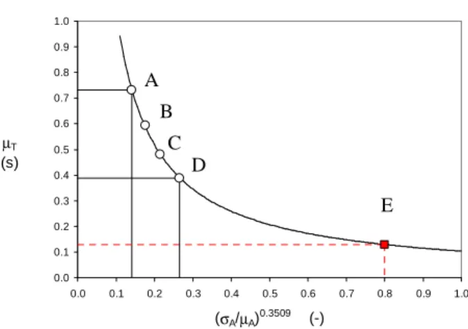
Scale condition D = 40.64cm 0.0 0.1 0.2 0.3 0.4 0.5 0.6 0.7 0.8 0.9 1.0 0.0 0.1 0.2 0.3 0.4 0.5 0.6 0.7 0.8 0.9 1.0 (σA/µA)0.3509 (-) µT (s)

Figure 3. A plot of Equation 7 for the D=40.64cm scale condition, where exponent p is -0.3509. ABCD are Fitts’ actual data points.

Point E is an arbitrary extrapolation on the same trade-off function.

Figure 3 plots Equation 7 for the case D=40.64cm, whose best fit is µT=0.1036/RVE 0.3509 (r²=.9992, see Figure 1), with the curve extrapolated on both sides of the actual range of x values. It is easy to see that the rectangle obtained by drawing straight horizontal and vertical lines to the axes from any point of the curve has a constant surface area (if y=q/x, then xy=q). This area is no other than the coefficient q of Equation 7, whose estimate in that particular scale condition is 0.1036s.

8

Needless to say, essentially the same flat curves obtain whether q is plotted against RVE or RTT.

A B

C D

(6)

5 The rectangle’s surface area is the same not only for Fitts’ four data points, but also for any point of the extrapolated curve like point E.

4.3. Resource Allocation: Strategic Imbalance

It is important to realize that different points along the curve of Figure 3 correspond, for a given amount of resources, to different degrees of imbalance between the concurrent time- and error-minimization efforts. While the product xy (the rectangular surface area in the figure) is conserved all along the curve, reflecting the limitation of resources, the ratio y/x (the rectangle’s aspect ratio) changes gradually, reflecting different resource-allocation options. For any data point of the curve the actual strategic imbalance (SI) of Ps can be quantitatively characterized by this aspect ratio, that is,

SI = µT / RVE-p. (9)

Since relative variable error RVE = σA/µA, we may write

SI = µT / (σA/µA)-p. (10)

With this definition of the aspect ratio (which we arbitrarily chose to compute as y/x rather than x/y), SI increases in Figure 3 from right to left: the more cautious (and the slower) the movement, the higher the SI. Thus the SI index correlates positively with—is an index of—the relative strength of the error-minimization component of the effort.

y = 0.5211x-0.7561 R2 = 0.9823 y = 0.4401x-0.8522 R2 = 0.9957 y = 0.3308x-0.7114 R2_{= 0.9986} y = 0.4102x-0.6095 R2_{= 1} 0 1 2 3 4 5 6 0.0 0.2 0.4 0.6 0.8 1.0

Relative target tolerance RTT = W/D (-) Strategic imbalance SI = mT/RME^-p (s) D=5.08 D=10.16cm D=20.32cm D=40.64cm

Figure 4. SI as a function of RTT in Fitts’ data.

Figure 4 shows the dependency of SI, which characterizes the actual strategy of Fitts’ Ps, upon RTT, the geometrical characteristic of the target layout which Fitts manipulated as an attempt to control his Ps’ strategy. This dependency is highly non-linear, confirming that the target-layout manipulation technique that Fitts introduced in his 1954 study actually provided him with mediocre control over the resource allocation strategy of his Ps.

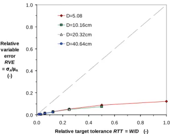
That mediocrity is also visible in Figure 5, which plots RVE, a characterization of performance, as a function of RTT, a characterization of the target layout. Although Fitts varied the tolerance over a very large range indeed (in fact up to the point where the two targets touched each other, i.e., W/D=1 or

W=D),9 RVE hardly exceeded 10% in the most tolerant

condition.

9

Using the reciprocal protocol, the condition W=D, which yields a Shannon ID of 1, corresponds to the highest possible level of tolerance. If W≥D, hence ID>1, the two targets overlap [8].

0.0 0.2 0.4 0.6 0.8 1.0 0.0 0.2 0.4 0.6 0.8 1.0

Relative target tolerance RTT = W/D (-) Relative variable error RVE = σσσσA/µµµµA (-) D=5.08 D=10.16cm D=20.32cm D=40.64cm

Figure 5. RVE as a function of RTT (the dashed line represents the theoretical case where RVE=RTT).

Back to Figure 4, notice the intriguing suggestion that Fitts’ Ps had two different strategic attitudes in the face of four different movement scales. Considering RTT<25%, where the

x ranges covered by the four curves substantially overlap, thus

making it possible to compare SIs for geometrically-similar target layouts, it seems that Fitts’ Ps had about the same set of strategic imbalances in the two larger-scale conditions D=20 and 40cm, while they apparently had another, more cautious set of strategies in the two smaller-scale conditions D=5 and 10cm. This finding, whose statistical reliability cannot of course be tested, might have resulted from the fact that large speeds cannot be attained over small amplitudes.

It should be remarked that if the pattern is quite conspicuous in the plot of Figure 4, it is virtually undetectable in the classic plot of µT vs. ID. Also note that it could not have been deduced from our previous observation that the resource pool was maximal in Fitts’ Ps for 10cm movements (Figure 2)— the aspect ratio (the quotient of µT/RVE-p) and the surface area (the constant product q=µT*RVE–p) of the rectangles of Figure 3 are two independent quantities.

4.4. Discussion

The foregoing shows that Fitts' classic data can be satisfactorily interpreted as a trade-off between two negative utilities, time and error. Thus, not only can we view Fitts' law as the demonstration that throughput—the inverse of the law’s slope, whose dimensions are bits/s—is conserved as the task

ID is made to vary, we can just as well view the law as

evidence that a certain pool of effort resources is conserved in the people across the variation of strategic imbalance. Both the information theoretic approach and the trade-off approach may help us understand Fitts' law.

5. SOME FRESH DATA: TIME/ERROR TRADE-OFF IN A NEW VARIANT OF FITTS TASK

This section reports a very simple experiment which only varied task instructions so as to induce a systematic variation of the Ps’ strategic imbalance in the face of the concurrent

(7)

time- and error-minimization efforts. Movement amplitude was invariably a comfortable 150mm.10

Among our motivations for running a fresh experiment was the fact that Fitts’ [2] individual data are not available. From the standpoint of trade-off theory, one expects some quantities—notably the coefficient q of Equation 5—to behave as within-individual constants while at the same time varying from participant to participant. Also of considerable interest is the variability of the strategic imbalance among and within individuals. Whether experimenters manipulate the target layout, as has been customary since Fitts, or speed/accuracy instructions, they face human beings with idiosyncratic strategic styles. No two participants will identically interpret instructions to move, say, as fast as possible; no two participants will show the same degree of flexibility in response to changing instructions.

Our discussion of Fitts’ data above did not refer to less-than-total resource exploitation, assumption #4 of our trade-off theory, whose illustration or testing require individual data. Below we will see that this assumption is quite useful to estimate individual trade-offs.

There were two notable differences between our protocol and Fitts’. The first is that our aiming task was discrete, rather than reciprocal, our Ps having to return to a fixed home position after each aimed movement. This option makes it possible to clarify the status of our temporal and spatial variables. Whereas in the reciprocal protocol µT is the time it takes not only to carry out a movement, but also to evaluate the error inherited from the previous movement and to prepare the next [3], in the discrete protocol µT measures the duration of a pure movement-execution process. The meaning of the movement’s endpoint spread σA is also interpretable more safely in the discrete case, that variability being generated just by the execution of the movement, whereas in the reciprocal case σA must also reflect, to some unknown extent, the variability of the start point [3]. Finally, one should perhaps recall that most pointing actions in real world of HCI are of the discrete sort. The other notable difference is that we did not specify tolerance W, just specifying target distance D by displaying two lines indicating the start point and the desired endpoint of the movement. The target being displayed as a single line, we manipulated the balance between the two concurrent minimization efforts by means of different sets of instructions. Such an approach offered us a chance to explore the full range of SIs. Experimenters, never knowing in advance the upper and lower extremes of the Ps’ strategic imbalance, choose their ranges of ID more or less arbitrarily. We asked our Ps to cover the whole spectrum of imbalances between µT and RVE, from the case of maximum speed to the case of maximum accuracy.

10

This experiment is part of a larger project aimed at understanding the interaction of the difficulty and scale factors in simple aimed movement performance.

5.1. Method

Speed-Accuracy Instructions

We used five sets of instructions: 1) Max speed, 2) speed emphasis, 3) speed/accuracy balance, 4) accuracy emphasis, and 5) max accuracy. In the max-speed condition the Ps were to just minimize movement time, the only requirement regarding accuracy being to refrain from committing a systematic error: no matter the dispersion of movement endpoints, Ps were just to manage to terminate their movements at about the target on average. At the other extreme, the max-accuracy instructions asked Ps to try to bring the cursor exactly to the target (zero pixel error), making as many corrective sub-movements and taking as much time— but not more—as needed. These two extremes being defined, we simply inserted three intermediate levels of instructions, one unbiased (speed/accuracy balance) and two biased (speed emphasis, accuracy emphasis). The ordinal level of this metric (with no assumption about the separating intervals) [23] was not a concern in this study, focused on the mutual relation of two random variables, µT and RVE.

Apparatus and Setup

The experiment involved a 1280x1024-pixel screen and a Wacom Intuos3 digitizing tablet connected to a PC running Linux Ubuntu. The screen permanently displayed two vertical lines extending from top to bottom, located 150mm apart, which marked the start point (left) and the target (right) of the movement. Both lines were 1-pixel thick and appeared in red color over a white background. Also displayed was a mobile 1-pixel thick cross-hair cursor, black in color, whose motion was controlled by the stylus. The tablet being used in absolute mode with a control-display gain of 1, the hand had to move 150mm from its home position for the crosshair to reach the target line.

The P was seated at a table supporting the Wacom tablet and the screen, with a viewing distance of about 50 cm. During initial warm up trials the Ps (all right-handers) were allowed to optimize the orientation of the tablet in the horizontal plane to facilitate the execution of the required left-to-right movement. They typically chose to slightly tilt the tablet in the counterclockwise direction. On the tablet was secured a horizontal 8-mm thick plastic ruler, along which the stylus tip was to be slid, allowing a strictly one-dimensional hand movement. The ruler offered a mechanical stop at its left end so that the start position of the stylus was standardized to the nearest screen pixel. To help initial positioning, an OK message appeared on the screen when the crosshair coincided with the start line.

We developed our own software, using Lib USB, for tablet-data acquisition, to minimize display latency relative to tablet events and to exploit the full resolution of the device (5080dpi). The tablet coordinates were translated into pixels using floating values to maximize visual-feedback accuracy. The sampling frequency of the tablet revolved about 100 Hertz (minimum 85 Hz, maximum 125 Hz).

Task and Movement Measurement Algorithms

To begin each trial the P immobilized the screen crosshair at the start line by positioning the stylus on the tablet at the ruler

(8)

7 stop for a few seconds. When ready, the P moved the stylus to the target position by sliding it against the ruler, finishing up with a dwell, then lifted the stylus and, after a few seconds rest, proceeded to the next trial. The movement start point obviously corresponded to the place and instant where the crosshair left its home position while exhibiting positive (rightward) acceleration. Determination of the movement

endpoint in time and space was a more subtle issue and

detailed explanations about the offline algorithm that would serve were part of the instructions received by the Ps.

We used two different criteria, depending on the instructions condition. For the max-speed condition, it was made clear to the Ps that the algorithms was going to take the first zero-crossing of instantaneous velocity as the movement endpoint, thus ignoring any subsequent episode of velocity, whether deliberate (a corrective sub-movement) or accidental (e.g., a mechanical rebound due to the elasticity of the arm). For the other four instructions conditions (which explicitly mentioned an accuracy component), the movement endpoint was defined as the beginning of the last dwelling period in the kinematic record, meaning that the algorithm would take into account all corrective sub-movements, if any. The criterion for dwell identification was the crosshair remaining stationary for at least 100ms at least 50mm away from the home position.

Procedure

Sixteen volunteers participated (all right-handers, median age=27.5 years, interquartile range=2.5, four females). The experiment consisted of 25 blocks of 15 movements, each block being run with a given set of instructions. All five instructions were presented in one order, ascending or descending, the order being reversed from one group of five blocks to the next. The experiment was run individually and lasted about 40mn, including 10mn warm up.

5.2. Results and Discussion Systematic Error, Variable Error

On average over all Ps mean aiming error (µΑ-150mm) was less than 1 screen pixel in all instructions conditions but the max-speed condition, where we found a consistent but rather small 5.5mm overshoot error (t15=4.504, p<.0005). It is fair to say that Ps constantly aimed to the target and that, as expected, it was their variable error σΑ/µA that was influenced, along with µT, by the variation of instructions.

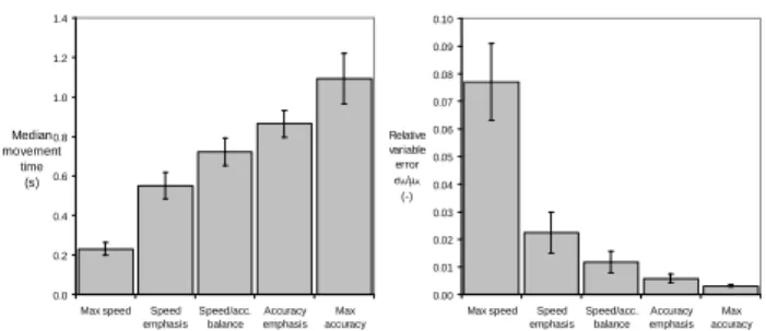
Effect of Instructions on Movement Time and RVE.

With increasing emphasis on accuracy, RVE decreased non-linearly, while µT lengthened about linearly (Figure 6). Although the max-speed instructions allowed any spread of movement endpoints, RVE hardly reached 8%, a finding reminiscent of Fitts’ data (see Figure 5).

0.0 0.2 0.4 0.6 0.8 1.0 1.2 1.4

Max speed Speed emphasis Speed/acc. balance Accuracy emphasis Max accuracy Median movement time (s) 0.00 0.01 0.02 0.03 0.04 0.05 0.06 0.07 0.08 0.09 0.10

Max speed Speed emphasis Speed/acc. balance Accuracy emphasis Max accuracy Relative variable error σA/µA (-)

Figure 6. The effect of instructions manipulation on µµµµT and RVE, on average over all Ps. Error bars are 95% confidence limits

based on between-P standard deviations.

Convex Front of Performance

P3 y = 0.0634x-0.4724 R2 = 0.8721 0.0 0.2 0.4 0.6 0.8 1.0 1.2 1.4 1.6 0.00 0.02 0.04 0.06 0.08 0.10

Relative variable error = σA/µA (-)

Median movement time (s) P3 y = 0.0461x-0.5089 R2 = 0.972 0.0 0.2 0.4 0.6 0.8 1.0 1.2 1.4 1.6 0.00 0.02 0.04 0.06 0.08 0.10

Relative variable error = σA/µA (-)

Median movement

time (s)

Fi gure 7. Panel A: a power curve (dashed line) was fitted to all the data points delivered by the P; the data points under the curve (filled discs) were then selected. Panel B: a power curve was fitted

to the selected data points, providing an approximation of the convex front of performance.

Assumption #4 of our trade-off theory, less-than-total resource exploitation, will help understand Figure 7, which illustrates for one representative P the trade-off between µT and RVE. Plotting the whole set of data points, one per trial block, for that P (Figure 7A), the best fit was a power function, with a substantial amount of noise, hence a moderately impressive r² of .87. The Ps having tried to minimize both µT and RVE in different proportions, we may liken their data points with particles attracted to the West and to the South by two magnetic fields whose respective strengths are modulated by instructions. Viewing the scatter as a mixture of forerunning and dawdling particles, we resorted to a simple dichotomous criterion assuming that the forerunners and the dawdlers were the data points under and above the curve, respectively.11 If the

11

We thank Eric Lecolinet for suggesting this simple solution.

A

(9)

resource pool is limited (assumption #3) then forerunners must have been constrained by a hard wall—the very trade-off curve we are looking for, which conceptually is no other than the borderline that separates in the equation space the region of the doable (above the curve) from the region of the

undoable (below). That hard wall must have prevented

forerunning data points from spreading any further in the South-West direction. But there must be dawdlers (assumption #4) and that constraint must have affected them to an attenuated extent. The data is quite consistent with this view. As shown in the lower graph of Figure 7, restricting the fit to the subset of forerunners improved the fit considerably (r² rising in the example considered from .87 to .97).

In fact this result was observed in all 16 Ps: with the fit restricted to forerunners, the r² improved on average from .852 to .972 (Student t15=8.83, p<.0001). In contrast, restricting the fit to the data points resting above the first curve (i.e., selecting the dawdlers) did not improve the fit whatsoever, the

r² changing on average over all Ps from .852 to .853 (t15=0.03,

p=.97). This outcome is congruent with the view that the data

points near the South-West quadrant of the convex hull of the scatter are those which, being most constrained by the resource limitations, are the most informative. This particular subset, indicative of the P’s best performance and which we call the convex front of performance, is our focus in the rest of this report.

Logarithmic, Exponential, and Power Fits

We tested the simple two-coefficient models that can accommodate the convex-down curvature evident in all our µT vs. RVE trade-off functions, the logarithmic, the exponential, and the power equation. Fitting the three candidate models to the full individual data sets (i.e., to the 25 pairs of measures originating from all trial blocks) resulted in the power model doing best in 10 cases (mean r²=.853 over all Ps), the exponential model doing best in four cases (mean r²=.803) and the log model in two (mean r²=.803). In general, the log and the exponential equation (most blatantly) failed due to insufficient curvature. Fitting the three models again to the convex-front data, the power model turned out to provide the best fit for all but one (P11) of our 16 Ps, with the r² now ranging between .923 and .992 (mean r²=.972, to be compared with .937 and .880 for the log and the exponential model, respectively). Therefore we retained the power equation

µT=q*RVE p for modeling the trade-offs.12

A Closer Look at Individual Exponents: Evidence for a One-Coefficient SQRT Relation

Thus, a simple power relation turned out to describe quite accurately the time/error trade-off in both Fitts’ data and our

12

The µT vs. RVE relation involves two random variables neither of

which is ‘dependent’ or ‘independent’. In such a case the so-called standard major axis method of curve fitting is known to be preferable over traditional linear regression, which measures errors only along the vertical y axis [21]. Here both methods yielded nearly identical estimates (not surprisingly, given the very high correlations found in

log-log plot between µT and RVE [21]), and so we judged it

superfluous to depart from the ordinary least-square method.

own, despite our different experimental protocol. Most interestingly, the exponent p of the best-fitting power model was similar, considering the two scales conditions of Fitts’ study that approximately corresponded to ours. In Fitts’ data the exponent was -0.54 for D=10cm and -0.38 for D=20cm (Figure 1); in our data, with D=15cm, the exponent was -0.47 on average. We further inquired into this issue by asking how the exponent varied with the goodness of fit and with the value taken by q, the other adjustable coefficient of Equation 5 (see Figure 8).

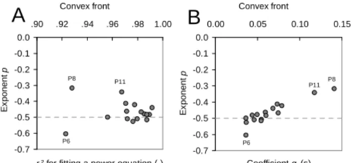
To reiterate, any individual P produces a mixture of good and poor performance (assumption #4), but there is an infinity of ways of performing poorly and in principle only the best (convex-front) performance of that P is informative. It should be realized that as one switches from a within- to a between-individual logic this argument works just the same. Different individuals being unequally able (or willing) to fully concentrate on a repetitive movement task, there is every reason to focus on the data of the best performers in one’s quest for a consistent quantitative law. A remarkable suggestion emerges from the data: (i) the better the fit of the power model, the closer the exponent to -1/2 (Figure 8A), and (ii) the smaller the value of the P’s coefficient q (i.e., the better the performer, as explained in Section 4.2), the closer the exponent to -1/2 (Figure 8B). Three individual estimates of the exponent diverged appreciably from -1/2, namely those delivered by P6, P8, and P11 (p=-.60, -0.34, and -0.32, respectively), but these happened to be the sample’s least credible estimates. P6 and P8 were two Ps for whom the power fit was distinctively worse than average (see Figure 8A). As for P11, we can see in Figure 8B that this P ranked 15th/16 for performance, next to P8, who ranked last—a further reason to moderately trust P8’s data.

Convex front -0.7 -0.6 -0.5 -0.4 -0.3 -0.2 -0.1 0.0 .90 .92 .94 .96 .98 1.00

r ² for fitting a power equation (-)

E x p o n e n t p P6 P8 P11 Convex front -0.7 -0.6 -0.5 -0.4 -0.3 -0.2 -0.1 0.0 0.00 0.05 0.10 0.15 Coefficient q (s) E x p o n e n t p P8 P11 P6

Figure 8. The exponent p of Equation 5 plotted (A) against the r² of the power fit and (B) against the value of coefficient q. Each

data point corresponds to an individual P.

Thus, focusing on the best performance (i.e., the convex-front of performance) of our best performers (actually 13 of our 16 Ps), we found that the trade-off of µT and RVE can be satisfactorily modeled in our data by a square-root equation with a single adjustable constant:

µT = q * RVE-1/2 or

µT = q / SQRT(σA/µA) (11)

where the multiplicative constant q is information about the amount of resources invested by each participant.

(10)

9

Constant Resource Pool and Variable Strategic Imbalance

To the extent that Equation 11 is a true description of the time/error trade-off in our simple aimed-movement task, it is also true, to the same degree of approximation, that the quantity q=µT*SQRT(σA/µA) is conserved within individual Ps across the variation of strategic imbalance (Section 4.2), and that the strategic imbalance can simply be quantified as the variable ratio SI=µT/SQRT(σA/µA) (Section 4.3).

P3 y = 0.0489x R2 = 0.9612 0.0 0.2 0.4 0.6 0.8 1.0 1.2 1.4 1.6 0 5 10 15 20 25 30 RVE-1/2 (-) Median movement time (s) P3 y = 0.0038x + 0.0458 R2 = 0.0731 0.00 0.01 0.02 0.03 0.04 0.05 0.06 0.0 0.5 1.0 1.5 Median movement time (s)

q = µT*RVE 1/2 (s)

A

B

Figure 9. Example, in one participant, of (A) the fit of the one-coefficient model of Equation 11 and (B) the approximate conservation of q across a considerable variation of µµµµT.

Figure 9, which uses the data from the same P as Figure 7, gives an example of the fit obtained with the one-coefficient model of Equation 11 and of the within-individual conserva-tion of q across the variaconserva-tion of µT. The orderly pattern visible in panel A was the rule. On average over the 13 Ps whose data had proved reliable (all but P6, P8, and P11), the r² for Equation 11 was .964 (.889<r²<.986), meaning that the fit was virtually as good with Equation 11 as with the more flexible two–coefficient model of Equation 5 (mean r²=.967, .891<r²<.987). Panel B displays a scatter plot with some noise but no evidence of any correlation between q and µT. The point being made in this figure is that µT failed to exert any consistent influence on coefficient q despite a considerable 7-fold variation. Indeed, considering our 13 reliable data sets, the slope of this relation (-0.0034s on average) did not significantly depart from zero (t12=-1.42, p=.182, two-tailed). Figure 10 shows the trade-off curves of two individual Ps whose q coefficients took distinctively different values. It is easy to see that P12 invested more resources in the task than did P13 (q=0.0425 and 0.0621, respectively). But the graph, by exhibiting different distributions of data points along their respective curves, also reveals that P12 and P13 had different

strategic preferences for resource allocation. In response to

our max-accuracy instructions P13 climbed his curve higher than P12 did his (SImax=22.5 vs. 18.9), and in response to our

max-speed instructions he did not explore his curve as far down as P12 did his (SImin= 1.07 vs. 0.35). Thus the comparison of two individual Ps delivers two pieces of evidence: beside the fact that P12 invested more resources than P13, he was more speed-biased.

0.0 0.2 0.4 0.6 0.8 1.0 1.2 1.4 0.0 0.1 0.2 0.3 0.4 0.5 SQRT(RVE ) (-) Median movement time (s) P13: µT = 0.0621 RVE -1/2 r ² = .978 P12: µT = 0.0425 RVE -1/2 r ² = .971

Figure 10. Comparing two individual trade-off curves.

6. IMPLICATIONS FOR HCI AND BASIC RESEARCH The trade-off approach to Fitts' law helps understand that target-acquisition performance, whose relevance to HCI research is obvious [12], is an inherently two-dimensional object whose complete description requires both an intensive and a qualitative characterization. If the intensive aspect is explicitly addressed by the throughput, reminiscent of the coefficient q of our trade-off analysis, apparently the information theoretic framework has little to say about the qualitative aspect. The fact that the speed/accuracy strategic balance is variable has been considered a worrisome complication calling for a certain correction—the substitution of effective to nominal width [1,12]—so as to end up with a single synthetic measure of performance. The correction being done, the throughput is quite insensitive to substantial variations of the speed-accuracy imbalance [4,13]. But the fact that throughput (or the coefficient q of our trade-off analysis) is not influenced by strategic variations does not mean that these variations are unimportant—a conclusion that a rapid reading of [13] might suggest. The cognitive set controlled by speed-accuracy instructions, which strongly modulates movement times and endpoint spreads, is obviously an important factor. This factor does not influence throughput, but it does influence another aspect of performance, the SI. The one-dimensional reduction to throughput has a cost. Suppose for example that, comparing two interaction techniques A and B, one finds more throughput with technique A in the presence of more errors. The conclusion that A outperforms B may be correct, assuming an appropriate adjustment for errors, but a full half of the story has been erased by the adjustment procedure. In some research contexts (e.g., where safety matters critically), it may be very useful to not ignore that different interface arrangements or interaction technique may induce different speed/accuracy imbalances in their users.

The trade-off and the information theoretic approaches are certainly not incompatible with each other, as recognized in practice by Fitts and Radford [4], who (although they did not

(11)

theorize on strategic imbalance) did manipulate speed-accuracy instructions. Indeed the right-hand side of Equation 11 rewritten as log2(µT) minus a constant = -½ log2(σA/µA) can be viewed to display bits of information. But the left-hand side of this equation, as already hinted above, is likely to call for a model involving joules of energy. Thus, one intriguing outcome of this trade-off analysis is the suggestion that information theory should certainly participate in, but probably will not suffice to wholly account for the empirical phenomenon known as Fitts' law.

7. ACKNOWLEGMENTS

This research has been supported by Institut Telecom, with a Carnot post-doctoral fellowship to HBO and a Futur et

ruptures PhD grant to STP, and by Ubimedia. We thank Eric

Lecolinet, Olivier Rioul, Fabrice Rossi, and Vincent Hayward for stimulating discussions and advice.

8. REFERENCES

1. Crossman, E.R.F.W. (1956). The measurement of perceptual load.

Unpublished PhD thesis, University of Birmingham, England. 2. Fitts, P.M. (1954). The information capacity of the human motor

system in controlling the amplitude of movement. Journal of Experimental Psychology, 47, 381-391 (reprinted in Journal of Experimental Psychology: General, 1992, 121(3), 262-269). 3. Fitts, P.M. & Peterson, J.R. (1964). Information capacity of

discrete motor responses. Journal of Experimental Psychology, 67, 103-112.

4. Fitts, P.M. & Radford, B.K. (1966). Information capacity of discrete motor responses under different cognitive sets. Journal of Experimental Psychology, 71, 475-482.

5. Guiard, Y. (2001). Disentangling relative from absolute movement

amplitude in Fitts’ law experiments. CHI’2001. New York: ACM Press, 315-316.

6. Guiard, Y. (2009). The problem of consistency in the design of Fitts' law experiments: Consider either target distance and width or movement form and scale. Proc. of CHI'2009. New York: Sheridan Press, 1908−18.

7. Guiard, Y. & Ferrand, T., 1998. Effets de gamme et optimum de difficulté spatiale dans une tâche de pointage de Fitts. Science et Motricité, 34, 19-25.

8. Guiard, Y. & Olafsdottir, H.B. (2010). What is a zero-difficulty movement? A scale of measurement issue in Fitts' law research. Submitted manuscript (a free-access copy is available on hal.archives-ouvertes.fr).

9. Hoffmann, E.R. (1996). The use of dimensional analysis in

movement studies. Journal of Motor Behavior, 28 (2), 113-123. 10. MacKenzie, I.S. (1991). Fitts' law as a performance model in

human-computer interaction. PhD thesis available online: http://www.yorku.ca/mack/phd.html.

11. MacKenzie, I. S. (1989). A note on the information-theoretic basis for Fitts' law. Journal of Motor Behavior, 21, 323-330. 12. MacKenzie, I.S. (1992). Fitts' law as a research and design tool in

human-computer interaction. Human-Computer Interaction, 7, 91-139.

13. MacKenzie, I.S. & Isokoski, P. (1988). Fitts’ throughput and the speed-accuracy tradeoff. Proc. of CHI'2008. New York: ACM Press, 1633−1636.

14. Meehl, P.E. (1997). The problem is epistemology, not statistics. In L.L. Harlow, S.A. Mulaik, and J.H. Steiger (Eds.), What if there

were no significance tests? (pp. 393-425). Mahwah, NJ: Erlbaum. Seehttp://www.tc.umn.edu/~pemeehl/169ProblemIsEpistemology.pdf.

15. Meyer, D. E., Smith, J. E. K., Kornblum, S., Abrams, R. A., & Wright, C. E. (1990). Speed-accuracy trade-offs in aimed movements: Toward a theory of rapid voluntary action. In M. Jeannerod (Ed.), Attention and performance XIII (pp. 173-226). Hillsdale, NJ: Erlbaum.

16. Plamondon, R., & Alimi, A.M. (1997). Speed/accuracy trade-offs in target-directed movements. Behavioral and Brain Sciences, 20, 279-349.

17. Rosenbaum, D. A. & Gregory, R. W. (2002). Development of a method for measuring moving-related effort: Biomechanical considerations and implications for Fitts’ Law. Experimental Brain Research, 142, 365-373.

18. Roberts, S., & Pashler, H. (2000). How persuasive is a good fit? A comment on theory testing. Psychological Review, 107, 358-367. 19. Schmidt, R.A., Zelaznik, H.N., Hawkins, B., Frank, J.S., & Quinn, J.T. (1979). Motor-output variability: A theory for the accuracy of rapid motor acts. Psychological Review, 86, 415-451.

20. Shannon, C.E. (1948). A Mathematical Theory of

Communication. Bell System Technical Journal, 27, 379-423 and 623-656.

21. Smith, R.J. (2009). Use and misuse of the reduced major axis for line-fitting. American Journal of Physical Anthropology, 140, 476-486.

22. Soukoreff, R. W., and MacKenzie, I. S. (2009) An informatic rationale for the speed-accuracy tradeoff. Proc. of SMC’2009. New York: IEEE, 2890-2896.

23. Stevens, S.S. (1946). On the theory of scales of measurement. Science, 103, No. 2684, 677-680.

9. APPENDIX: GLOSSARY OF IMPORTANT VARIABLES Task geometry

Target distance D (cm)

Target width or tolerance W (cm)

Relative target distance RTD = D/W (-)

Relative target tolerance RTT = W/D (%)

Elemental movement measures

Movement time T (s)

Movement amplitude A (cm)

Movement error E = A−D (cm)

Movement statistics

Mean movement time µT (s)