HAL Id: hal-00687316
https://hal.archives-ouvertes.fr/hal-00687316
Submitted on 12 Apr 2012
HAL is a multi-disciplinary open access archive for the deposit and dissemination of sci-entific research documents, whether they are pub-lished or not. The documents may come from teaching and research institutions in France or abroad, or from public or private research centers.
L’archive ouverte pluridisciplinaire HAL, est destinée au dépôt et à la diffusion de documents scientifiques de niveau recherche, publiés ou non, émanant des établissements d’enseignement et de recherche français ou étrangers, des laboratoires publics ou privés.
Data Cleaning: Approach for Earth Observation Image
Information Mining
Avid Roman Gonzalez, Mihai Datcu
To cite this version:
Avid Roman Gonzalez, Mihai Datcu. Data Cleaning: Approach for Earth Observation Image Infor-mation Mining. ESA-EUSC-JRC 2011 Image InforInfor-mation Mining: Geospatial Intelligence from Earth Observation Conference, Mar 2011, Ispra, Italy. pp.117-120. �hal-00687316�
DATA CLEANING: APPROACHES FOR EARTH OBSERVATION IMAGE INFORMATION
MINING
Avid Roman-Gonzalez, Mihai Datcu
German Aerospace Center (DLR), Oberpfaffenhofen, 82234 – Wessling, Germany
ABSTRACT
Actually the growing volume of data provided by different sources some times may present inconsistencies, the data could be incomplete with lack of values or containing aggregate data, noisy containing errors or outliers, etc. Then data cleaning consist in filling missing values, smooth noisy data, identify or remove outliers and resolve inconsistencies. In more general definition, data cleaning is a task to identify something that is unusual and try to correct it.
1. INTRODUCTION
The data and information are not static; they are object of various processing steps, for example: data acquisition, data delivery, data storage, data integration, data retrieval, data analysis, etc. All these processes can lead to changes in data and inconsistencies may occur, these changes and inconsistencies are called as something unusual. For to detect something unusual, we look at the following string:
“MRQA9”, we build a mental model as what is usual and
what is unusual, after 4 letters is not expected a number. The satellite image also could be affected by some unusual or artifacts. In figure 1 we show some examples of artifacts, in (a) we can see the existence of vertical line, a dropout; (b) shows other type of defects in bottom left as prolongations.
(a) (b)
Fig. 1 Some Examples of Artifacts: (a) Shows the existence of vertical line, death line. (b) Defects in bottom left.
The artifacts detection was approached in [4] using Rate-Distortion analysis and Normalized Compression Distance [3]. In this article, we extend these methods: The first method uses Lossy Compression to calculate the Rate-Distortion Function. The Rate-Rate-Distortion analysis allows us to
evaluate how much the data was distorted, we further develop and asses the method in [4] based on the analysis of the lossy compression error for variable compression factor. Second method uses the Lossless Compression to calculate Normalized Compression Distance (NCD), the NCD is a method proposed in [5] to determine the similarity between two files using a distance measure based on Kolmogorov complexity. These both methods are compared to third method based on image quality metrics.
The paper is structured as follow. Section II presents an overview on the theory on which these methods are based. Section III shows practical applications in artifacts detection in optical images. Finally section IV reports our conclusions.
2. METHODS DESCRIPTION
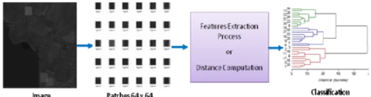
The general schema block for the three methods is presented in figure 2. The first step is take the satellite image and divide it into patches of 64x64 pixels, with these patches we calculate the distance matrix or feature vector, depending the method, we present 3 methods: The first one is using rate-distortion analysis, the second one is based on compression similarity metrics and the third one is based on image quality metrics. Finally we applied a hierarchical classification method to cluster and identify the patches with artifacts. In the next subsection we describe the different processes for feature extraction, distance computation and classification.
Fig. 2 General Block Diagram for Artifacts Detection
2.1. Feature Extraction Using Rate – Distortion Analysis
The Rate-Distortion (RD) Function is given by the minimum value of mutual information between source and receiver under some distortion restrictions. Plotting Experimental RD Curve, we can do an analysis of the image.
For the artifacts detection, we propose to use the RD function obtained by compression of the image with different compression factors and examine how an artifact can have a high degree of regularity or irregularity for compression. The feature extraction process is done as the blocks diagram shown in Fig. 3, we compress each patch with different compression factors, then decompress the image and calculate the error for each compression factor, based on the errors we compose a features vector.
Fig. 3 Feature Extraction Process for Rate-Distortion Analysis: we compress each patch with different compression factors, then decompress the patch and
calculate the error for each compression factor, based on the errors we compose a features vector.
2.2. Distance Computation Normalized Compression Distance (NCD)
The Normalized Compression Distance NCD is introduced in [5], is a distance metrics between 2 data using the approximation of K(x) with C(x) = K(x) + k, the length of the compressed version of x obtained by a lossless compressor C plus an unknown constant k. The NCD is calculated by:
(
,)
(
,)
{
m in( ) ( )
{
( ) ( )
,}
}
m ax , C x y C x C y N C D x y C x C y − =Where: C(x, y) represents the size of compressed file obtained by the concatenation of x and y.
The NCD represents how different are 2 files, facilitating the use of this result into various applications into a parameter-free approach [3, 6].
With the patches, we calculate the distance matrix between them using NCD. That is D = {dij}; i = 1…N, j =
1…N; where N is the number of patches and dij is the NCD between patch pi and patch pj.
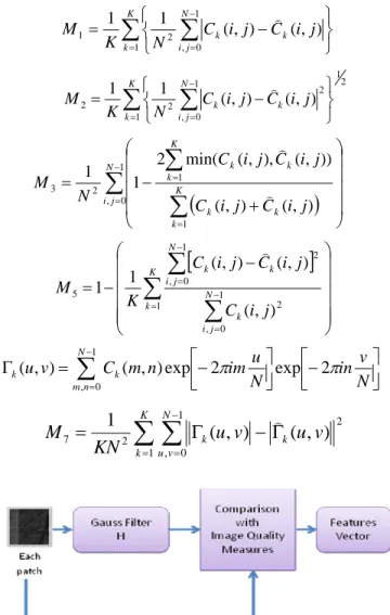
2.3. Feature Extraction Using Image Quality Measures
For this method we take the work presented in [9] where the authors present a technique for steganalysis using image quality metrics. We use this method because it has a similar concept to RD, where a variation in the compression factor could has a similar result as a filter. The feature extraction processes for this method is to compare the original patch to the patch after apply a Gaussian filter. The Gaussian filter was chosen as H(m,n) = K*g(m,n) where
}
2
/
)
(
exp{
)
2
(
)
,
(
m
n
πσ
2 1m
2n
2σ
2g
=
−−
+
is the 2-DGaussian kernel and 2 1/2
) ) , ( (
∑ ∑
− = m n g m n K is thenormalizing constant, the aperture of the Gaussian filter was set to
σ
=5 with a mask size 3x3. For the comparison weuse the image quality metrics like: Mean Absolute Error
(M1), Mean Square Error (M2), Czekanowski Distance (M3), Image Fidelity (M5), Normalized Cross-Correlation (M6) and Spectral Magnitude Distortion (M7). In figure 4 we present
the feature extraction using image quality metrics.
Fig. 4 Feature Extraction Process Using Image Quality Metrics
2.4. Classification
For the classification step, we apply a hierarchical classification method. The Dendrogram is a type of graphical representation of data as a tree that organizes the data into subcategories that are dividing in others to reach the level of detail desired, this type of representation allows appreciating clearly the relationship between data classes. To plot the dendrogram we use the Euclidean Distance method. Also we use de k-means algorithm.
3. CASE STUDIES AND RESULTS
To evaluate the proposed methods, we will use different case studies with artificial artifacts introduced manually; and with real artifacts introduced by the sensor itself.
∑
∑
= − = ⎭⎬ ⎫ ⎩ ⎨ ⎧ − = K k N j i k k i j C i j C N K M 1 1 0 , 2 1 (, ) (, ) 1 1 )∑
∑
= − = ⎭⎬ ⎫ ⎩ ⎨ ⎧ − = K k N j i k k i j C i j C N K M 1 2 1 1 0 , 2 2 2 (, ) (, ) 1 1 )(
)
∑
∑
∑
− = = = ⎟ ⎟ ⎟ ⎟ ⎠ ⎞ ⎜ ⎜ ⎜ ⎜ ⎝ ⎛ + − = 1 0 , 1 1 2 3 ) , ( ) , ( )) , ( ), , ( min( 2 1 1 N j i K k k k K k k k j i C j i C j i C j i C N M ) )[
]
⎟⎟ ⎟ ⎟ ⎟ ⎠ ⎞ ⎜⎜ ⎜ ⎜ ⎜ ⎝ ⎛ − − =∑
∑
∑
= − = − = K k N j i k N j i k k j i C j i C j i C K M 1 1 0 , 2 1 0 , 2 5 ) , ( ) , ( ) , ( 1 1 )∑
− = ⎥⎦ ⎤ ⎢⎣ ⎡− ⎥⎦ ⎤ ⎢⎣ ⎡− = Γ 1 0 , 2 exp 2 exp ) , ( ) , ( N n m k k N v in N u im n m C v uπ
π
∑ ∑
= − =Γ
−
Γ
=
K k N v u k ku
v
u
v
KN
M
1 1 0 , 2 2 7(
,
)
(
,
)
1
)
3.1. Case Study 1 – Validation with Synthetic Data for RD Analysis:
For this part we have simulated the aliasing artifact in the image, the image is processed in 2 ways; in the first one we apply the downsampling process in order to obtain an image with aliasing. In the second one we apply a low pass filter before downsampling in order to obtain an image without aliasing. Finally we combine some parts of these images.
After applying the methodology presented to the image with aliasing, the results for the aliasing detection is shown in Fig. 5 where we present the areas that contain the aliasing.
(a) Image with Aliasing (b) Aliasing Detection Fig. 5: (a) Shows a satellite image with artificial aliasing. (b) Shows the
aliasing detection using RD analysis.
3.2. Case Study 2 – Validation with Actual Data for RD Analysis:
Another result of artifacts detection with RD, it is the dropout detection shown in Fig. 6, In this case it is a SPOT image containing actual artifacts, was analyzed and the detection is done correctly.
(a) © CNES (b)
Fig. 6 Dropout (SPOT). (a) Some electronic losses during the image formation process create these randomly saturated pixels. The dropouts often follow a line pattern (corresponding to the structure of the SPOT sensor). (b)
Artifact is detected.
3.3. Case Study 3 – Validation with Synthetic Data for NCD-based Method:
We introduce two types of artifacts with different intensities in such a way to study their behavior; these artifacts are introduced manually, in the first instance we introduce strips with different levels of intensity, which is done is to increase the grayscale value of the satellite image in the desired positions. For the aliasing simulation, we also use different values of down sampling. The introduction of artificial artifacts is made with different intensities to assess the sensitivity of the detection method.
To evaluate the proposed method, we made a study of detection sensitivity with different levels of intensity of the artifact, so also this study has been done in different environments such as: sea, forest and city. So our database contains images of different environments with different types of artifacts at different levels of intensity. Finally, after applying the method to our database, we can see the results expressed as percentage of success in table 2.
3.4. Case Study 4 – Validation with Actual Data for NCD-based Method:
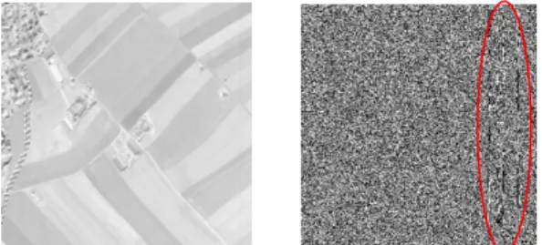
For images with real artifacts, we considered images acquired by the ROSIS sensor provided by the German Aerospace Center (DLR); these data are hyperspectral images of 7946x512 pixels, 115 bands and 16 bits/pixel. We work with subscene of 512x512 pixel. First thing, we make a manual analysis to determine the location of artifacts, thus we detect strips in the last two bits as shown in Fig. 7.
Fig. 7 Bit by Bit Analysis for Strips Detection in the ROSIS Image: we can see the strips in the last bits.
After applying the proposed method, the results are not encouraging and are shown in the following table 1:
Table 1 Result for Artifacts Detection in Actual Data
These low performance may be because the strips are presented in the last bits are indexed not detected.
Given these results, the next experiment is to take directly the binary image containing strips, divided it into 64x64 patches and each patches convert to a string with values of 0s and 1s, then calculate the Normalized Compression Distance with these strings and finally apply the hierarchical classification. For doing the conversion to string, we analyze a horizontal scanning and vertical scanning. As each patch has 64x64 pixels and to form the text string we order either row or column after another, then finally each text string will be formed by 4096 values.
The results after applying the proposed approach are: a total mixture for horizontal scanning and a 81.25% of successful for vertical scanning. The results for vertical scanning are much better because the strips have the same vertical orientation.
3.5. Case Study 5 – Validation with Synthetic Data for Image Quality Metrics:
For the images with artificial artifacts, we use the same data described in section 3.3. After applying the method to our database, we can see the results expressed as percentage of success in table 2.
3.6. Case Study 6 – Validation with Actual Data for Image Quality Metrics:
Another result of artifacts detection with image quality metrics is shown in figure. 8, in this case it is a SPOT image containing actual artifacts, and the detection is done.
Fig. 8 Artifacts Detection Using Image Quality Metrics
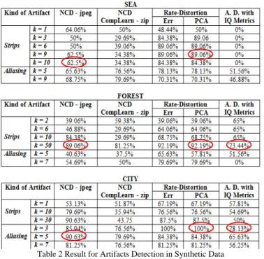
Table 2 Result for Artifacts Detection in Synthetic Data
In the table 2, we present the results for the different environment: sea, forest and city, with the strips and the aliasing artifacts in different intensities. The NCD calculation was made using different compressors as JPEG and zip. The intensity of the strips for detection is lower in the sea. The better detection of aliasing occurs in the city because the image bandwidth is wider.
4. CONCLUSIONES
About the artificial artifacts, we can appreciate that the strips have an acceptable possibility to be detected in a sea environment from an intensity of k = 10, however in the forest and the city environment with intensity k = 30. The aliasing can be detected in a city environment, but not at sea or in the forest images, due to de city’s bandwidth is widest than the sea and forest. The detection of artifacts is done best way depending on the environment we are working, at sea and in the field is easier to detect the strips but not so the aliasing, while in the city and the forest is easier to detect aliasing. About the real artifacts, we can see that there aren’t good results and this may be because the strips are presented in the last bits and can not be detected. The acceptable results are found with scanning vertically, column by column as the strips also have the same orientation.
In all cases, the method using image quality metrics do not give good results.
5. ACKNOWLEDGMENT
The ROSIS data was made available by DLRs OpAIRS service (http://www.OpAiRS.aero). The authors very much acknowledge the support of Dr. Martin Bachmann from DLR. This work is in the frame CNES / DLR / TELECOM ParisTech - Competence Center on Information Extraction and Image Understanding for Earth Observation.
6. REFERENCES
[1] A. Roman-Gonzalez, M. Datcu, “Parameter Free Image Artifacts Detection: A Compression Based Approach”, Proc. SPIE Remote
Sensing, vol. 7830, 783008, Toulouse, France, Sep. 2010.
[2] J. Hyung-Sup, W. Joong-Sun, K. Myung-Ho, L. Yong-Woong, “Detection and Restoration of Defective Lines in the SPOT 4 SWIR Band”, IEEE Transaction on Image Processing, 2010.
[3] D. Cerra, A. Mallet, L. Gueguen, M. Datcu, “Algorithmic Information Theory Based Analysis of Earth Observation Images: an Assessment”, IEEE Geosciences and Remote Sensing Letters. [4] A. Mallet, M. Datcu, “Rate Distortion Based Detection of Artifacts in Earth Observation Images”, IEEE Geosciences and
Remote Sensing Letters, vol. 5, N° 3, pp. 354-358, July 2008.
[5] M. Li, X. Chen, X. Li, B. Ma, P. M. B. Vitanyi; “The Similarity Metric”, IEEE Trans. Inf. Theory, vol. 50, N° 12, pp. 3250-3264. [6] E. Keogh, S. Lonardi, Ch. Ratanamahatana, “Towards Parameter-Free Data Mining”, Department of Computer Science and
Engineering, University of California, Riverside.
[7] R. Cilibrasi, P. M. B. Vitanyi; “Clustering by Compression”,
IEEE Trans. on Inf. Theo., vol. 51, N° 4, April 2005, pp 1523 - 1545.
[8] T. Tao, A. Mukherjee, and R.V. Satya, “A search-aware JPEG-LS variation for compressed image retrieval”, Intelligent
Multimedia, Video and Speech Processing, (2004), 169-172.
[9] I. Avcibas, N. Memon, B. Sankur; “Steganalysis Using Image Quality Metrics”; IEEE Transaction on Image Processing, vol. 12, N°2, Feb. 2003, pp. 221-229.