HAL Id: hal-03147898
https://hal-imt-atlantique.archives-ouvertes.fr/hal-03147898
Submitted on 21 Feb 2021
HAL is a multi-disciplinary open access
archive for the deposit and dissemination of
sci-entific research documents, whether they are
pub-lished or not. The documents may come from
teaching and research institutions in France or
abroad, or from public or private research centers.
L’archive ouverte pluridisciplinaire HAL, est
destinée au dépôt et à la diffusion de documents
scientifiques de niveau recherche, publiés ou non,
émanant des établissements d’enseignement et de
recherche français ou étrangers, des laboratoires
publics ou privés.
Device-Free People Counting Using 5 GHz Wi-Fi Radar
in Indoor Environment with Deep Learning
Ali El Amine, Valery Guillet
To cite this version:
Ali El Amine, Valery Guillet. Device-Free People Counting Using 5 GHz Wi-Fi Radar in Indoor
Environment with Deep Learning. 2020 IEEE Globecom Workshops (GC Wkshps): IEEE
GLOBE-COM 2020 Workshop on AI-driven Smart Healthcare (GC 2020 Workshop - AIdSH), IEEE, Dec 2020,
Taipei, Taiwan. �10.1109/GCWkshps50303.2020.9367393�. �hal-03147898�
Device-Free People Counting Using 5 GHz Wi-Fi
Radar in Indoor Environment with Deep Learning
Ali El Amine, Valery Guillet
Orange Labs, 1 Rue Louis et Maurice de Broglie, 90000, Belfort France Email:{ali.elamine; valery.guillet}@orange.com
Abstract—People counting plays an important role in many people-centric applications including crowd control, traffic man-agement and smart home energy manman-agement. With the ad-vancements in wireless sensing, it is now possible to intelligently sense the presence of people with wireless signals. Yet, a lot of challenges arise when Wi-Fi solutions are used for counting humans due to the uncertainty of the states in the environment. In this paper, we propose a novel 3D-Convolutional Neural Network (3D-CNN) architecture able to extract features from range-Doppler images to count the number of people present in an indoor environment by detecting their movements. We generate the range-Doppler images from a Celeno Wi-Fi pulse Doppler radar that uses the 5 GHz frequency band. To the best of our knowledge, this work is the first to count people based on a Wi-Fi Doppler radar. Our experimental results show that our deep learning model is able to estimate the number of people for up to four with an average accuracy of 89%.
Index Terms—Wi-Fi sensing, Doppler radar, presence detec-tion, people counting, deep learning
I. INTRODUCTION
Wireless sensing has received great attention in recent years. A lot of research efforts have revealed the sensing ability to recognize human activity, human identification, localization and beyond [1]. In particular, Wi-Fi environmental sensing plays an important role in the areas of health care, smart home, security and virtual games [2]. Among its various applications, people counting in indoor environments is of great interest to many people-centric, Internet of Things (IoT) applications including crowd control, traffic management and smart home energy management. Classical solutions to this problem are devised into two broad categories: image-based and non-image based solutions. Image-based counting solutions use specific hardware (e.g., camera) for people counting. In addition to being an expensive approach, this method has many drawbacks such as Line-of-Sight (LOS) requirement, lighting conditions requirements, and privacy problems.
Non-image based solutions perform counting based on wire-less signals (infrared, ultrasound, Wi-Fi, etc.). These solutions alleviate the previous drawbacks as they can perform in a Non-Line-of-Sight (NLOS) environment. They do not require lighting conditions, they significantly reduce privacy concerns and they are economical and practical solutions since they do not require additional equipment to be installed. Among the different radio technologies, Wi-Fi emerges as a promising and effective solution in wireless sensing. This can be best achieved by utilizing the Channel State Information (CSI)
values captured from Wi-Fi signals highlighting the different multipaths distortions based on human activity [3].
Feature extraction combined with Machine Learning (ML) models have received great attention in activity recognition and people counting during the last decade [1]. In particular, Deep Learning (DL) has paved the way as an appealing option in extracting useful features for different classification tasks while adapting to real-world imperfections. One of the earliest work on counting people using DL is found in [4]. The authors explored the correlation between people count (up to five people) and Wi-Fi CSI variations using a fully connected feed-forward neural network with two hidden layers. Their model achieved an accuracy of 78% when neither action nor position restrictions are imposed on the volunteers. The work was extended in [5] where a Convolutional Neural Network (CNN) combined with Long Short Term Memory (LSTM) DL architecture was adopted to resolve the dependencies of number of people and CSI. With this architecture, the accuracy was improved to84.6%. In another work on counting humans using DL, the authors in [6] leveraged Recurrent Neural Network (RNN) to count people walking in an indoor environment by placing the transmitter and receiver behind the walls. The authors tested their system for a total number of 10 simultaneous people reaching an accuracy of 59%. In a similar work, the authors in [7] proposed a CNN architecture to extract features from the received CSI information to link it with the number of moving people. The model achieved an average accuracy of 71% for counting up to five people in different indoor locations.
The above mentioned work considered the relationship between CSI waveforms and people counting. Doppler radar systems have been also proposed to capture the human body motion. Opportunistic monitoring using passive Doppler radar was considered in [8]. With a wireless energy transmitter and a radar sensor, the authors generated Doppler spectrograms to extract the person’s activity from a set of actions. In a similar work, the authors in [9] studied Doppler scalograms for different human activities including walking, clapping, falling and sitting.
In this paper, we propose a novel 3D-CNN model able to extract features from range-Doppler images to count the number of people present in an indoor environment. The experiment is carried out using a commercial Wi-Fi pulse Doppler radar that operates in the 5 GHz frequency band. This radar can be integrated in any classical Wi-Fi access point that
uses the same frequency band. To the best of our knowledge, this work is the first to count people based on Doppler and micro-Doppler frequencies measured from movements such as walking and breathing. In contrast to [4]–[7] that measure the CSI between two locations, in this paper, and for the best of our knowledge, we propose the first solution to use a single device able to generate range-Doppler images for feature extraction to classify people count. We achieve an accuracy better than the ones attained in the previous presented literature. Different from [8], [9] that limit the work to one person only, our model extends the presence detection up to four people.
The rest of the paper is organized as follows. Section II describes the pulse Doppler radar used in this work and details the signal processing steps. In Section III, we detail the architecture of the 3D-CNN used in this work. The evaluation of our proposed model is reported in Section IV. Finally, Section V concludes the paper.
II. SYSTEM DESIGN AND IMPLEMENTATION
In this section, we first present the hardware description and the performance of the pulse Doppler radar used in this work to sense the environment. Then, we detail the signal processing steps performed to generate the range-Doppler images capturing the presence of people. Finally, we describe the experimental setup carried out in this work. The overview of the system design block diagram is summarized in Fig. 1.
MIMO Radar Transceiver
Sensing the Environment
Data Sampling
Collect CSI Data
Reduce Spectral Leakage Generate Range-Doppler Images Extract Features 3D – CNN Classification Wi -Fi Radar CSI Pr ocessi n g P eople C oun ting
Fig. 1: Block diagram system overview.
A. Wi-Fi radar overview and performance
The measurements in this paper have been carried out by an active pulse Doppler radar based on Celeno 802.11ac Wi-Fi chipset in the 5 GHz frequency band [10]. This radar contains one transmitter and 4 receiving antennas. Its antenna elements geometry corresponds to a uniform linear array. For calibration purposes, a reference channel that usually contains the signal from source is acquired by one of the receiving antennas’ port. The radar uses 80 MHz of bandwidth to generate Wi-Fi radio pulses with a period of 1 ms (can be modified), then it collects
0 20 40 60 80 100 120 140 160 180 192
Sample number (Range)
-60 -50 -40 -30 -20 -10 0 |h| dB Rx 1 Rx 2 Rx 3
Fig. 2: Average power delay profile over the different receive antennas.
the back scattered echos in the form of CSI data of the shifted Doppler frequencies. We summarize in Table I the radar radio characteristics.
TABLE I: Celeno radar radio characteristics.
Carrier frequency 5.54GHz
Bandwidth 80MHz
Pulse duration 40 µ s
Pulse period 1ms
EIRP 11 dBm
Directivity 30◦lobe at 3 dB and 60◦lobe at 6 dB
Celeno radar has the potential to detect objects as far as 10 meters in LOS and 5-6 meters in NLOS depending on obstruct-ing materials. It has a range resolution of∆r = c/2B = 1.875 m. The Doppler frequency resolution∆Fdis a function of the
observation time frame Tf rame, ∆Fd = 1/Tf rame. In order
to be able to detect people with different movement activities (e.g. walking and breathing), a fine Doppler resolution is required. In the next section, we discuss how to adjust the Doppler resolution to detect the sensitivity from different actions.
B. CSI processing
The presence of people in an indoor environment can be detected using pulse Doppler radar by either sensing move-ment or detecting breathing. These features can be obtained by measuring the Doppler frequencies received from the reflected signals of moving objects (in this case people). We divide the signal processing into two parts:
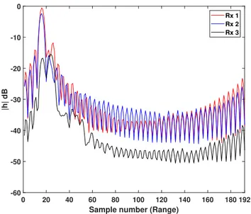
1) Reduce spectral leakage: We plot in Fig. 2, the average
Power Delay Profile (PDP) over the different receive antennas during a total time duration T . The radar samples its total 80 MHz bandwidth into 48 sample points. We then add zero padding of size 3 × 48 to resolve the waveform signal. This results in 48 × 4 = 192 samples. These samples can also be
0 20 40 60 80 100 120 140 160 180 192
Sample number (Range)
-70 -60 -50 -40 -30 -20 -10 0 |h| dB Rx 1 Rx 2 Rx 3
Fig. 3: Average power delay profile over the different receive antennas with Hanning window on the range axes.
interpreted as range or distance points. The received signals are calibrated by the reference transmitted signal and the average PDP is calculated as follows:
ri(τ ) = hi(τ ) × s(τ ) = hi(τ ) × r4(τ ) (1a)
Ri(F ) = FFT(ri(τ )) = Hi(F ) × R4(F ) (1b)
PDP(τ ) = hi(τ ) = iFFT(Hi(F )) (1c)
whereτ is the propagation delay, riis the received signal at the
i-th receiver, s is the transmitted pulse and hi is the channel
gain between the object and receiver i. Since the transmitter is directly connected to the port ofr4,s(τ ) can be substituted
byr4(τ ). FFT and iFFT are the Fast Fourier Transform and
inverse Fast Fourier Transform, respectively.
In order to reduce spectral leakage and side lobes that might be masking actual echos, we apply a window in the frequency domain for the range axes. The choice of the window has a major impact on the side lobes attenuation, and thus on reducing the spectral leakage. Many windows exist in the literature with different characteristics (i.e., highest side lobe level, side lobe fall-off, etc.) [11]. In our work, we applied a Hanning window on the range axes. This window has a wide peak and low side lobes. In Fig. 3, we plot the average PDP with a Hanning window applied on the range axes. Compared to Fig. 2, we can observe the different delayed echos that were masked by the side lobes due to spectral leakage.
For each transmitted pulse, the radar captures the CSI from its returned signal in the form of amplitudes and phases over the 192 sample points. For a total ofN transmitted pulses, we denote by Ci the captured CSI by the i-th receiver. It can be
expressed as follows: Ci= (a1,1, φ1,1) . . . (a1,192, φ1,192) .. . . .. ... (aN,1, φN,1) ... (aN,192, φN,192) (2)
where an,d and φn,d are the amplitude and phase received
from then-th pulse at the d-th distance point.
A range-Doppler imageIi can be generated from the above
captured Ci by performing a Fast Fourier Transform (FFT)
overTf rameconsisting ofF pulses. A Chebyshev window is
applied in the time domain with a 75 dB side attenuation to reduce spectral leakage and capture low Doppler frequencies that are around the DC component. We can write a range-Doppler image as follows:
Ii= |b1,1| . . . |b1,192| .. . . .. ... |bF,1| ... |bF,192| (3)
where |bf,d| is the amplitude of the Doppler frequency fd at
distance pointd.
From the totalN transmitted pulses, we generate S Doppler images each containing F frequency bins. The number of images can be calculated as follows:
S =jN − F F
k
(4) These images will be used later as the input of our deep learning architecture.
2) Time-Frequency analysis: The Doppler images
gener-ated in the previous section are sampled in time. Thus, a sequence of these images show the variations of the Doppler frequencies in time. To address the time dependency varia-tions, we use Short Time Fourier Transform (STFT). The idea is to pass a sliding Chebyshev window over the received signal to capture the frequency components. The window of width Tf rameslides on the time axis with a step durationtstep.
In order to detect human presence, a high Doppler resolution is required to capture slow movements. Breathing for instance results in a Doppler frequency of less then 1 Hz. We set the radar sampling frequency fs = 200 Hz. We then set
the window size to F = 1024 pulses and a time step tstep= 130 ms. This is equivalent to a time frame duration of
Tf rame= 1024/200 = 5.12 seconds. This gives us a Doppler
frequency resolution of ∆fd = 1/Tf rame = 0.195 Hz with
a maximal Doppler frequency of fmax
d = ±fs/2 = ±100
Hz. Such resolution will allow us to capture low Doppler frequencies from respiration as well as higher frequencies from movements such as walking.
In order to reduce the process complexity of the deep learning process, we limit the size of the Doppler images to 64 frequency bins and 64 range points. This results in an image of size64×64. We do this by grouping different frequency bins to obtain a logarithmic scale on the frequency axes that spans low frequency components for micro movement detection (e.g., breathing detection) and high frequency components for macro movement detection (e.g., walking). We illustrate in Fig. 4 some examples of generated images from different scenarios.
C. Experimental setup and datasets collection
We conducted our experiment in an apartment living room representing a domestic indoor environment. The detail of the
5 10 15 20 25 30 35 40 45 50 55 60 64 Sample number (Range)
-60 -40 -20 0 20 40 60 Doppler frequency (Hz) 0 5 10 15 20 25 30 35 40
(a) Empty room
5 10 15 20 25 30 35 40 45 50 55 60 64 Sample number (Range)
-60 -40 -20 0 20 40 60 Doppler frequency (Hz) 0 5 10 15 20 25 30 35 40
(b) One sitting person
5 10 15 20 25 30 35 40 45 50 55 60 64 Sample number (Range)
-60 -40 -20 0 20 40 60 Doppler frequency (Hz) 0 5 10 15 20 25 30 35 40
(c) One walking person
5 10 15 20 25 30 35 40 45 50 55 60 64 Sampling number (Range)
-60 -40 -20 0 20 40 60 Doppler frequency (Hz) 0 5 10 15 20 25 30 35 40
(d) One sitting person and one walking person
10 20 30 40 50 60 Sampling number (Range) -60 -40 -20 0 20 40 60 Doppler frequency (Hz) 0 5 10 15 20 25 30 35 40
(e) Two sitting persons and one walking person
10 20 30 40 50 60 Sample number (Range) -60 -40 -20 0 20 40 60 Doppler frequency (Hz) 0 5 10 15 20 25 30 35 40
(f) Four walking persons
Fig. 4: Examples of different range-Doppler images with different scenarios.
room plan is described in Fig. 5. This room has furniture: a dining table, a small table, a bed, a closet, a desk and chairs. The furniture is all made from wood. The radar is placed on the floor as shown in the Fig. 5 and facing the area of interest. The blue dotted area represents the coordinates where people are allowed to move. The radar is placed in this location to have the area in interest in LOS.
We collected data samples from different scenarios. We conducted 12 cases of measurements: 1) empty room, 2) one sitting person, 3) one walking person, 4) two sitting persons, 5) one sitting person and one walking person, 6) three sitting persons, 7) one sitting person and two walking persons, 8) two sitting persons and one walking person, 9) four sitting persons, 10) four walking persons, 11) one sitting person and three walking persons and 12) two sitting persons and two walking persons.
We do not limit or force the volunteers to take fixed positions or fixed activities. The volunteers are free to move inside the dotted area with no restrictions on the distance between them.
III. 3D-CNNARCHITECTURE
This section highlights the deep learning architecture which learns from the constructed images the number of people present inside the room. This architecture is based on CNN and in particular 3D-CNN [12]. Radar Closet Table Desk Din in g table
The units are in cms
Fig. 5: Room plan and measurement locations.
CNN is a class of deep learning neural networks that is used in image processing and classification [13]. CNN networks have shown very good performances in objects recognition by automatically extracting features from raw inputs and ability to learn localized patterns through weights sharing and pooling. One important characteristic of CNN is that the extraction of features is shift-invariant. This gives CNN the ability to recognize patterns at different locations of the input [14]. This
Input images 64x64x38 64xC1 64x64x38 25xC1 32x32x18 16xC1 16x16x9 64xP1 32x32x18 25xP2 16x16x9 16xP3 8x8x4 1000xM1200xM2 5xM3 Classes 0 person 1 person 3 persons 4 persons 2 persons 3D-Conv 3x3x10 3D-Conv 3x3x9 3D-Conv 3x3x8
Fig. 6: 3D-CNN architecture illustrating the input images, the output classes and the different intermediate layers.
characteristic is important in our classification problem as the presence signal can happen at any period of time.
The main component of a CNN is the convolution layer. It is composed of several filters or kernels that are small in size. The goal of these filters is to extract features from the image that is the input of the network. In a 3D-CNN, The filters have the shape of (size 1, size 2, size 3) which is an matrix of weights, and each point in the filter is a neuron. These filters are applied to the input. In our problem, the input is a sequence of images. It has the shape of (Distance, Doppler frequency,
time). The output of the convolution layer is called feature
maps having a shape of (Distance, Doppler frequency, time,
filters number). The pooling layer acts as a down-sampling
layer to reduce the system computational complexity. We consider a CNN composed of 3 convolution layers. Each convolution layer is followed by a max pooling layer. The output of the last max pooling layer serves as input for a classical Multi-Layer Perceptron (MLP) network. The role of the MLP is to classify the extracted information (features map) from the previous convolution layers. We illustrate in Fig. 6 the architecture of our convolution network. The input consists of a sequence of 38 images, each having a size of 64x64. This size represents the points in Doppler frequency and distance. In other words, we have 64 Doppler frequencies and 64 distances points. The number of images or frames can be regarded as a time dimension. The convolution layers (C1,
C2andC3) consist of 64, 25 and 16 filters, respectively. Their
kernel sizes are 3 × 3 × 10, 3 × 3 × 9 and 3 × 3 × 8. Each convolution layer is followed by a max pooling layer (P1,P2,
and P3) of size (2 × 2 × 2). The output of the last pooling
layer (P3) enters an MLP network of size 1000 neurons and
then another MLP network of size 200. The output of the last MLP network (M3) is the output of our network identifying
to which class the input images belongs. In order to reduce overfitting, we add a dropout layer between the MLP layers with a value of 0.15. The choice of the hyperparameters are based on extensive simulations. These values resulted in having the optimal accuracy.
IV. EVALUATION AND RESULTS
In this section, we describe the datasets used for training and validation in our deep learning architecture. For training the 3D-CNN, we use the Keras library with TensorFlow 1.5 back-end in Python 3.6. The training and testing phase have been supported by two NVIDIA Quadro P5000 with CUDA Toolkit 9.1 and cuDNN 7.1 with a batch size set to 64.
A. Evaluation setup
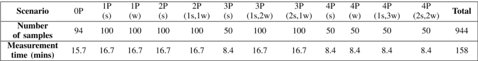
We consider 944 samples for training and validation. Each sample consists of 38 range-Doppler images. Given that the images are generated from sliding windows of size 5.12 seconds with a time step tstep = 130 ms, each sample of
38 images is 10.06 seconds long. We detail in Table II the measurements taken for the different scenarios. We refer to
0Pthe case of empty room (zero person), as for 1P, 2P, 3P and 4P the cases where there are one to four persons. Then, we distinguish between a person sitting on a chair (s) and a walking person (w). For each scenario, we conduct different measurements. The total amount of measurement time is158 minutes.
Because we have a limited number of training samples, we artificially increase our dataset by making translations on the range axes in the range-Doppler images. This is a possible solution since in this work we are not interested at what range (position) the frequencies were captured. Thus, we perform four translations for each image resulting in augmenting our dataset by a factor of four. Then, we adopt K-Fold cross validation method to train and validate the data collected. This method splits the collected data intoK sets. One of the k sets is used for testing (validation), while the remainingk − 1 sets are used for training. The cross validation is repeatedK times with each of the k sets is used exactly once as the validation data. The overall performance is then evaluated by averaging over theK sets. In this work, we set K = 5.
B. Benchmark algorithms
We compare our 3D-CNN architecture with two baseline methods: Fully Connected Back Propagation (FCBP) neural network and Gaussian Naive Bayes (GaussianNB). FCBP is a fully connected MLP neural network which contains a lot of tunable parameters that is suited for people counting. We use a FCBP with two hidden layers. The first hidden layer contains 300 neurons whereas the second hidden layer contains 100 neurons. The input layer is the sequence of 38 images vectorized and reshaped to one dimension vector of size64 × 64 × 38.
Naive Bayes model is a classical linear classification algo-rithm that belongs to the family of probabilistic classifiers [15]. It is a supervised learning method based on applying Bayes theorem with strong independence (naive) assumption between features. GaussianNB assumes that the collected data are distributed according to a Gaussian (or normal) distribution. Naive Bayes classifiers do not require a lot of data to train and they are simple to implement. The input of this model is similar to the FCBP model.
TABLE II: Summary of the measurements dataset from different scenarios. Scenario 0P 1P(s) (w)1P 2P(s) (1s,1w)2P 3P(s) (1s,2w)3P (2s,1w)3P 4P(s) (w)4P (1s,3w)4P (2s,2w)4P Total Number of samples 94 100 100 100 100 50 100 100 50 50 50 50 944 Measurement time (mins) 15.7 16.7 16.7 16.7 16.7 8.4 16.7 16.7 8.4 8.4 8.4 8.4 158 C. Results
In Table III, we compare the average classification accuracy obtained by our proposed 3D-CNN architecture with FCBP and GaussianNB. This average is obtained over the 5 exper-iments (Ex.#) from the 5-fold cross validation. From the ob-tained results, we observe that 3D-CNN outperforms the other two baseline models with an average accuracy of 89.62%, while FCBP and GaussianNB achieve 73.51% and 45.35%, respectively. The lower performance of the GaussianNB model is due to the assumption that the features are independent. Thus, it processes the range-Doppler images in the sample as one vector with independent data features. The importance of the correlation between the range-Doppler images in one sample can be well distinguished with the other two deep learning architectures as the average classification accuracy almost doubled. The accuracy achieved by FCBP shows that it is powerful enough to count people. However, 3D-CNN handles images sequence better by extracting features from the applied filters, and uses these features for classification. TABLE III: Classification accuracy obtained from our pro-posed 3D-CNN architecture and other baseline methods.
Architecture/
Method Ex. 1 Ex. 2 Ex. 3 Ex. 4 Ex. 5 Acc.
3D-CNN 89.15% 87.95% 92.19% 87.28% 91.52% 89.62%
FCBP 73.54% 69.84% 73% 78.83% 72.34% 73.51%
GaussianNB 42.72% 42.35% 47.6% 48% 46.1% 45.35%
We present in Fig. 7 the confusion matrix obtained from our 3D-CNN model describing the performance of our classifier. The horizontal axis corresponds to the actual class whereas the vertical axes corresponds to the predicted class.
V. CONCLUSION
In this paper, we present a novel DL model based on 3D convolutional networks to solve the problem of people counting with a pulse Doppler Wi-Fi radar. Taking into account the complexity of the environment and various cases such as sitting and walking people, we achieved a good counting accuracy of 89% for up to four people in LOS with no constraints on the actions taken by the volunteers. For future work, we focus on extending the model to sense human presence and count people in a NLOS scenario and to be able to track the positions of the people.
REFERENCES
[1] Abdullah Khalili, Abdel-Hamid Soliman, Md Asaduzzaman, and Alison Griffiths. Wi-fi sensing: Applications and challenges. The Journal of
Engineering, 2020. 0 1 2 3 4P 0P 0.92 0.01 0.07 0.00 0.00 1P 0.00 0.88 0.07 0.02 0.03 2P 0.04 0.01 0.87 0.06 0.02 3P 0.00 0.00 0.03 0.86 0.11 4P 0.00 0.00 0.01 0.00 0.99
Fig. 7: The confusion matrix for 3D-CNN network architec-ture.
[2] Oscar D Lara and Miguel A Labrador. A survey on human activity recognition using wearable sensors. IEEE communications surveys &
tutorials, 2012.
[3] Zheng Yang, Zimu Zhou, and Yunhao Liu. From rssi to csi: Indoor localization via channel response. ACM Computing Surveys (CSUR), 2013.
[4] Shangqing Liu, Yanchao Zhao, and Bing Chen. Wicount: A deep
learning approach for crowd counting using wifi signals. In 2017 IEEE International Symposium on Parallel and Distributed Processing with Applications and 2017 IEEE International Conference on Ubiquitous
Computing and Communications (ISPA/IUCC). IEEE, 2017.
[5] Shangqing Liu, Yanchao Zhao, Fanggang Xue, Bing Chen, and Xiang Chen. Deepcount: Crowd counting with wifi via deep learning. arXiv
preprint arXiv:1903.05316, 2019.
[6] Osama Talaat Ibrahim, Walid Gomaa, and Moustafa Youssef. Cross-count: A deep learning system for device-free human counting using wifi. IEEE Sensors Journal, 2019.
[7] Iker Sobron, Javier Del Ser, I˜naki Eizmendi, and Manuel Velez. A deep learning approach to device-free people counting from wifi signals. In International Symposium on Intelligent and Distributed Computing. Springer, 2018.
[8] Wenda Li, Bo Tan, and Robert Piechocki. Passive radar for opportunistic
monitoring in e-health applications. IEEE journal of translational
engineering in health and medicine, 2018.
[9] Mohammed Al-Rahbi. Human activity recognition using channel state information. 2019.
[10] Celeno Wi-Fi Doppler imaging technology. [Online]. Available:
https://www.celeno.com/wifi-doppler-imaging.
[11] Fredric J Harris. On the use of windows for harmonic analysis with the discrete fourier transform. Proceedings of the IEEE, 1978.
[12] Ian Goodfellow, Yoshua Bengio, and Aaron Courville. Deep learning. MIT press, 2016.
[13] Jianxin Wu. Introduction to convolutional neural networks. National Key
Lab for Novel Software Technology. Nanjing University. China, 2017.
[14] Qiang Yang, Zhi-Hua Zhou, Zhiguo Gong, Min-Ling Zhang, and Sheng-Jun Huang. Advances in Knowledge Discovery and Data Mining: 23rd Pacific-Asia Conference, PAKDD 2019, Macau, China, April 14-17,
2019, Proceedings. Springer, 2019.
[15] K Ming Leung. Naive bayesian classifier. Polytechnic University