Processing aortic and pulmonary artery
waveforms to derive the ventricle
time-varying elastance
David J. Stevenson∗ Christopher E. Hann∗ Geoffrey J. Chase∗ James Revie∗ Geoffrey M. Shaw∗∗
Thomas Desaive∗∗∗ Bernard Lambermont∗∗∗ Alexandre Ghuysen∗∗∗ Phillippe Kolh∗∗∗
Stefan Heldmann∗∗∗∗
∗Department of Mechanical Engineering, University of Canterbury,
Christchurch, New Zealand
∗∗Department of Intensive Care, Christchurch Hospital, Christchurch,
New Zealand
∗∗∗Hemodynamics Research Laboratory, University of Liege, Belgium ∗∗∗∗Department of Mechanical Engineering, TU Darmstadt, Germany
Abstract: Time-varying elastance of the ventricles is an important metric both clinically and as an input for a previously developed cardiovascular model. However, currently time-varying elastance is not normally available in an Intensive Care Unit (ICU) setting, as it is an invasive and ethically challenging metric to measure. A previous paper developed a method to map less invasive metrics to the driver function, enabling an estimate to be achieved without invasive measurements. This method requires reliable and accurate processing of the aortic and pulmonary artery pressure waveforms to locate the specific points that are required to estimate the driver function. This paper details the method by which these waveforms are processed, using a data set of five pigs induced with pulmonary embolism, and five pigs induced with septic shock (with haemofiltration), adding up to 88 waveforms (for each of aortic and pulmonary artery pressure), and 616 points in total to locate. 98.2% of all points were located to within 1% of their true value, 0.81% were between 1% and 5%, 0.65% were between 5% and 10%, the remaining 0.32% were below 20%.
Keywords: Cardiovascular system, Time-varying elastance, Model-based cardiac diagnosis,
Pressure waveform, Signal Processing, Intensive Care Unit, Porcine model 1. INTRODUCTION
In the Intensive Care Unit (ICU), cardiac disturbances are very difficult to diagnose and treat, which can lead to poor management of the circulation (Guyton and Hall (2000); Grenvik et al. (1989)). Left and right pressure-volume (PV) loops contain a large amount of information on cardiac function including all the states of filling, contraction, ejection and relaxation. From this data a cardiac elastance can be defined:
el(t) = Plv(t) Vlv(t) − Vd
(1) where
Vd≡ intercept of the end-systolic PV relation with the volume axis Plv(t) ≡ left ventricle pressure
Vlv(t) ≡ left ventricle volume
(2)
Derived by Suga and Sagawa (1974), it is commonly called time varying elastance, and provides a load-independent measure of heart function (Oommen et al. (2003); Suga et al. (1973); Senzaki et al. (1996)), while representing the cardiac muscle activation. Time varying elastance is
typically normalised to one, and the resulting shape can be used as the input or driver function into lumped parameter models of the cardiovascular system (Smith et al. (2004)). The shape of the driver function thus approximates the change in cardiac muscle activation over time, and implicitly contains information on the ventricle pressure and volume profiles. However, determining the parameter Vd requires an invasive vena cava occlusion manoeuvre, and the left and right ventricle pressures and volumes, which is invasive and ethically challenging to measure. Hence, they are not available as typical ICU care. Stevenson et al. (2010) developed a method to estimate the ventricle driver functions, based on pre-calculated, global correlations between the ventricle driver functions and less invasive measurements of the pulmonary artery and aortic pressure waveforms. These driver functions then provide the input into a previously developed eight chamber cardiovascular system (CVS) model (Starfinger et al. (2008)), as well as significant diagnostic information in relation to cardiac energetics. Hence, these estimates based on readily available data can have significant clinical potential.
The pre-calculated correlations map specific points on the aortic and pulmonary artery pressure waveforms to specific points on the driver function. The points on the driver function were chosen as a minimum set of points through which a smooth curve can be generated that captures the necessary dynamics of the actual driver function waveform. The locations on the pressure waveforms that map to the driver functions were found from known physiological con-nections and empirical relations (Stevenson et al. (2010)). They are shown briefly, without explanation, in Table 1 and Figures 1 and 2. This paper focus on the method of processing the pressure waveforms in order to locate the points required by the correlations, thus enabling these driver function estimates.
Fig. 1. Aortic pressure over one heart beat, including relevant points defined in Table 1, note that RS & MN are used only in locating other points
0 0.05 0.1 0.15 0.2 0.25 0.3 0.35 0.4 0.45 0.5 25 30 35 40 45 50 55 60 65
Fig. 2. Pulmonary artery pressure over one heart beat, including relevant points defined in Table 1, note that MX is used only as part of locating DN
2. CONCEPT
The concept behind this paper involves creating a set of correlations that map the less invasive metrics to the desired, more invasive metrics, where the correlations are later used to estimate the more invasive metrics. In this case, the correlation map aortic pressure, pulmonary artery pressure and global end diastolic volume to left and right ventricle time-varying elastance.
An illustration of this concept is given in Figure 3, while Figure 4 shows a more detailed picture. The process requires the pre-calculation of the correlations. To do this took a set of both the invasive and less invasive metrics must be available. From this set, correlations can be derived from known physiological connections, and empirically by lining up the two waveforms. To derive the empirical correlations, and (later) estimate the invasive metrics, a method for processing the waveforms must be developed. This method must be able to reliably and
accurately identify specific locations on these waveforms. This paper details that method.
Fig. 3. The concept of estimating an invasive metric using pre-calculated, global correlations
Fig. 4. Pictorial overview of the process of finding the real and approximate driver functions
3. METHODOLOGY
To enable driver function identification and its clinical outcomes, two pressure waveforms are processed to ex-tract specific points of time, value and gradient. These waveforms are the aortic pressure (Pao) and pulmonary artery pressure (Ppa). The accuracy and robustness of this processing is critical to the accuracy of the time-varying elastances built from the resulting data. A naming convention for these points of interest is defined in Table 1, and graphically in Figures 1-2 (Stevenson et al. (2010)).
Table 1. Naming convention
Left Right Description
el er driver function
Pao Pao aortic pressure
Ppa Ppa pulmonary artery pressure
DM P G driver maximum positive gradient
M N M N minimum point
M P G maximum positive gradient
LS left shoulder
M X M X maximum point
RS right shoulder
M N G maximum negative gradient
DN DN dicrotic notch
DC dicrotic crest
ta,b ta,b time of point b on waveform a
The processing method is described using Pao as the pressure waveform. However, the same approach is used for Ppa, except where stated.
The points of interest, shown in Figures 1-2, are located in the following order, M X, M N , DM P G, LS, M P G, DN ,
RS, and DC, where previously located points are used in the location of subsequent points.
Note that before processing Pao and Ppa, both waveforms were smoothed using a locally weighted 2nd
degree poly-nomial regression (loess) over a range of 0.04 seconds.
3.1 Shear Transformation
To facilitate the extraction of a number of points, a shear transformation is defined:
(t, X(t)) → (t, φshear(X(t))
φshear(X(t)) = X(t) + mt + c, t0< t < tend (3) The parameters t0 and tend are set depending on the region of interest. The parameters m and c are chosen such that φshear(X(t0)) = X(t0) and φshear(X(tend)) = X(t0) which leads to the following equations:
X(t0) + mt0+ c = X(t0) (4a) X(tend) + mtend+ c = X(t0) (4b) Solving(4a) and(4b) yields:
m= X(t0) − X(tend) tend− t0
c= t0(X(t0) − X(tend)) tend− t0
(5)
To better visualize this transformation, imagine a line from MN to MX (of Figure 1), rotated about MN so that this line is horizontal, while the time remains unchanged, e.g. a rotation and contraction that projects the line onto a horizontal surface (time). The effect of this transformation is to transform the point LS into a peak of a curve, and thus easier to locate. Figure 5 shows an example of this transformation. This shear transformation is applied to several regions to locate shoulders and changes of slope.
Fig. 5. the section from Figure 1 between M N and M X, before and after the shear transformation from(3).
3.2 M X, M N , and DM P G
M X is straight forward to locate as it is the global maximum of the waveform, the time of which is defined:
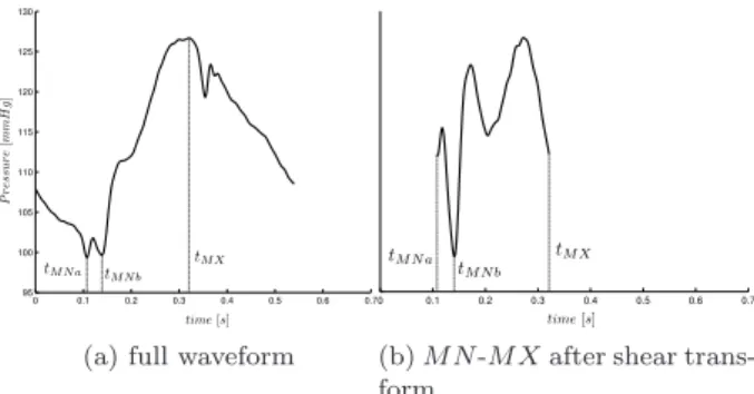
tM X ≡ time of maximum Pao (6) M N and DM P G occur in close proximity around the global minimum of the pressure waveform. M N is thought of as the minimum of the pressure. However, it is not always the global minimum as in some cases there exists a trough just before DM P G that is lower, and occasionally there exists a lower point in the second half of the waveform. Hence, it would be unreliable to locate M N as the global minimum.
Instead, a second property of M N is used, M N is located at the bottom of the steeply rising section from M N to LS, and M N always appears in the first half of the waveform. A shear transformation is applied to the section from the minimum (of the first half of the waveform) to M X, and the minimum of the transformed section is found. The difference in these to time points indicates which is the true M N , as illustrated in Figures 6-7.
0 0.1 0.2 0.3 0.4 0.5 0.6 0.7 95 100 105 110 115 120 125 130
(a) full waveform
0 0.1 0.2 0.3 0.4 0.5 0.6 0.7
(b) M N -M X after shear trans-form
Fig. 6. An example where M N is not the global minimum
0 0.1 0.2 0.3 0.4 0.5 0.6 0.7 110 115 120 125 130 135 140 145 150
(a) full waveform
0 0.1 0.2 0.3 0.4 0.5 0.6 0.7
(b) M N -M X after shear trans-form
Fig. 7. An example where M N is the global minimum First, locate the minimum of the first half of the waveform:
tM N a≡ time of minimum of first half of Pao (7) Define the section between tM N a and M X and pass it through the shear transformation of (3):
Pao,secA≡ {Pao(t) : tM N a< t < tM X} (8) tM N b≡ time of minimum φshear(Pao,secA) (9) A threshold is then applied to the distance between tM N a and tM N b, to select the real M N , defined:
errorPao ≡ tM N b− tM N a period (10) and tM N = tM N b, errorPao <0.025 = tM N a, otherwise (11)
The constant 0.025 was found empirically, and the final value of tM N in (11) gives good results in all cases. Note that for Ppa, a shear transformation is not required as the case of Figure 6 never occurs. Thus, the method simply calculates:
tM N ≡ time of global minimum Ppa (12) DM P Gis only needed for the Pao waveform and is found by applying the shear transformation of (3) to a small
neighbourhood to the left of M N . The specific section, and condition are defined:
Pao,secB≡ {Pao(t) : 3
4· tM N < t < tM N} (13) CE≡ (tM X− tM N) < period · 0.23 (14) Where the both fraction 3/4 and the constant 0.23 were empirically derived. The time tDM P G is then defined:
tDM P G≡ time of local maximum φshear(Pao,secB) (15) To account for some waveforms that have an early rise (which is consistent with shorter pressure pulse) tDM P G may be changed, as defined:
tDM P G≡ tM N, if CE
≡ tDM P G, otherwise (16)
3.3 LS and M P G
Both points LS and M P G are defined only for Pao. M P G is one of the most important features physiologically and clinically, and is commonly called dPaodtmax, which is well known to relate to ventricle contractility.
To locate LS a new section is defined:
Pao,secC ≡ {Pao(t) : tM N < t < tM X} (17) The simplest approach to finding LS would be to locate the maximum of φshear(Pao,secC), as in Figure 5. However, in a number of cases, the shear transformation produces a second, higher peak. For example, for a curve shape like Figure 2, this second, higher peak would be the second ‘bump’ between M N and M X, which is the wrong point. The solution is to find both local maxima then have a second criteria to distinguish the correct point. The first maximum is:
tLSa≡ time of maximum φshear(Pao,secC) (18) To account for the case of tLSa being the wrong point, which means it will be far up the waveform past LS, a section is defined:
Pao,secC2≡ {Pao(t) : tM N < t < tLSa} (19) For this case, the correct time of LS should be:
tLSb ≡ time of maximum φshear(Pao,secC2) (20) However, in a number of cases tLSais correct, which would mean tLSbis a false point that lies somewhere between MN and LS in Figure 1. To account for both of these cases the solution is: tLS= tLSa, (tLSa− tLSb) < period 20 = tLSb, otherwise (21) where tLSaand tLSb are given by (18) and (20).
The first condition of (21) is due to the curve from MN to LS being close to sigmoidal so that when tLSa is the correct point, tLSb is always very close and within a 20th of the period. In the case where tLSais incorrect, and thus tLSbis the correct point, tLSa− tLSb is much greater than 20th
of the period, and, in fact, is commonly between a 10th
to a 5th
of the period.
Once tLS is found, the time point corresponding to MPG in Figure 1 is defined: tM P G≡ time of maximum { d dt(Pao(t)) : tM N < t < tLS} (22) 3.4 DN, RS and DC
Note that RS and DC are only defined for Pao.
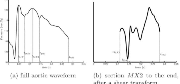
The dicrotic notch (DN) in Figure 1 occurs at the close of the aortic value, which corresponds to the end of ejection. The simplest way of defining tDN would be to use tM X from (6) and to compute the minimum of the shear transformed data for tM X < t < tend, where tend = period. However, in a number of cases near the end of the trial, when the pig is near death, the maximum peak of Pao occurs between the two points LS and MX in Figure 1. Physiologically this phenomenon is likely due to the twisting of the ventricle becoming abnormal and dysfunctional. In practice, it is probably too late to save a patient if this occurs. However, for completeness, this scenario is accounted for in the following method. Figure 8 shows an example of this case.
0 0.05 0.1 0.15 0.2 0.25 0.3 0.35 95 100 105 110 115 120 125
(a) full aortic waveform
0 0.05 0.1 0.15 0.2 0.25 0.3 0.35
(b) section M X2 to the end, after a shear transform
Fig. 8. An example where the M X needs to be moved to correctly locate DN
To ensure that the correct value of tM N is obtained for the case of Figure 8, an estimate of the first local minima just after tM X is empirically determined from all similar cases to Figure 8. The result is:
tDN a≡ tM N+ period
5 (23)
and this time point is shown in Figure 8a. There is some variation in the position of tDN a, but, importantly it always occurs before the true dicrotic notch and after the first local minima following TM X. A second estimate of DN is defined:
tDN b≡ time of local minimum DNshear (24) where:
DNshear ≡ φshear(Pao,secD) (25) Pao,secD≡ {Pao(t) : tM X2< t < tend} (26) tM X2≡ time of maximum {Pao(t) : tDN a< t < tend}
(27) Note that DNshear is smoothed using a ‘loess’ method over a 0.06 second range, this is to eliminate any fine oscillation in the waveform which would affect the location of tDN c. There are a handful of cases where tDN astill does not match the correct location for DN , due to a later, lower trough as in Figure 9. However it is not sufficient to just take the first local min of DNshear as illustrated in Figure 10. To accommodate for these cases, an third possibility for DN is defined along with four conditions are defined to select between the first and lowest local minimum of DNshear:
0 0.05 0.1 0.15 0.2 0.25 0.3 0.35 100 105 110 115 120 125 130
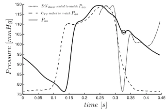
Fig. 9. An example of where the lowest local minimum of DNshear does not match the real location for DN (shown with a circle). Note that the start and end of DNshear are not the same due to heavy smoothing.
0 0.05 0.1 0.15 0.2 0.25 0.3 0.35 0.4 0.45 75 80 85 90 95 100 105 110 115 120
Fig. 10. In this case the lowest local min of DNshearis the real DN (shown with a circle) but the first local min is not. CA≡ DNshear(tDN c) > DNshear(tM X2) CB ≡ (tDN c− tM X2) < 0.15 · period CC≡ DNshear(tDN c) − DNshear(tDN b) Pao(tM X) >0.02 CD≡ tDN c− tM X2<0.11 · period (29)
The motivation behind these conditions are as follows: CA prevents the choice of a local minimum, above the starting point of the transformed data, see Figure 10. However, this is only the wrong point if it occurs early, hence CB and the use them together. CC prevents the choice of a local minimum that is to much above the lowest local minimum, again this is only the wrong point if it occurs early, hence CD and the use of CC and CD together.
From the conditions in (29), the final location for DN is defined:
tDN= tDN b, if (CA AND CB) OR (CC AND CD)
= tDN c, otherwise (30)
For Ppa, the final value is simply:
tDN = tDN b (31)
tDNis then adjusted to the local minimum within a range of period · 0.04 seconds, if such a minimum exists. This is necessary due to the fact that the minimum is located based on a sheared waveform and hence is slightly off the minimum of the true waveform.
The remaining values, RS and DC, are only defined for Pao. The value of tRS is defined:
tRS ≡ time of maximum φshear(Pao,secE) (32) where:
Pao,secE≡ {Pao(t) : tM X < t < tDN} (33)
Finally, the last section is defined:
Pao,secF ≡ {Pao(t) : tDN < t < tDN+ 0.05} (34) and the crest after the dicrotic notch is found by:
tDC≡ time of maximum Pao,secF (35)
3.5 Summary
A summary of the overall process for Pao is defined: Step 1. find tM X using (6)
Step 2. find tM N with (7)-(11) for Pao or (12) for Ppa Step 3. find tDM P G with (13)-(16)
Step 4. find tLS with (17)-(21)
Step 5. find tM P Gbetween M N and LS, (22) Step 6. find tDN with (23)-(30)
Step 7. find tRS with (32)-(33) Step 8. find tDC using (34)-(35)
A summary of the overall process for Ppa is defined: Step 1. find tM X using (6)
Step 2. find tM N with (7)-(11) for Pao or (12) for Ppa Step 3. find tDN with (23)-(24) and (31)
4. RESULTS
The method presented in this paper was developed on a set of five pigs (51 waveforms) that were induced with pulmonary embolism (Desaive et al. (2005); Ghuysen et al. (2008)), and further developed on another five pigs (37 waveforms) that were induced with septic shock (Lamber-mont et al. (2003, 2006)).
The points for each waveform manually identified, after which the method was applied to the waveforms and assessed against the manually identified points. For the points (M N and DN ) required in the pulmonary artery waveform, the method located both points in 87 of the 88 waveforms to within the sample frequency of 200Hz. The method only missed a single point, DN , from one waveform. This waveform was as the start of the third pig of the sepsis cohort and is unique to the data set, both in the driver function measured and the pulmonary artery pressure waveform, shown in Figure 11, see Figure 2 for a more normal Ppa waveform. The reason that the method failed to identify the correct location for DN is the unusual second peak of Ppa, and the early decay of the driver function. 0 0.2 0.4 0.6 0.8 1 1.2 1.4 7 8 9 10 11 12 13 14 15 16
Fig. 11. Pulmonary artery waveform, alongside the match-ing driver function. The method failed to capture the correct DN in this case. The three circles are the identified points, from left to right M N , M X, DN . The real location for DN is marked by a square.
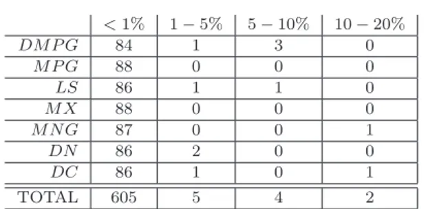
For each aortic pressure waveform, the method locates nine points. However, two of these, RS and M N , are only used in aiding the location of other points. Hence, the tolerance on their location is much larger than the other points. These two points were both located sufficiently to enable the method to progress in all 88 waveforms. Results for the other seven points are shown below in Table 2.
Table 2. Accuracy of the method: number of points grouped by accuracy of location
<1% 1 − 5% 5 − 10% 10 − 20% DM P G 84 1 3 0 M P G 88 0 0 0 LS 86 1 1 0 M X 88 0 0 0 M N G 87 0 0 1 DN 86 2 0 0 DC 86 1 0 1 TOTAL 605 5 4 2
A similar method (for locating the points on the pressure waveforms) was used to estimate the driver functions (Stevenson et al. (2010)) which produced excellent results comparing, for pulmonary embolism, the approximated driver functions to the measured driver functions, see Table 3, and correlations with R values ranging from 0.81 to 0.99 for the left side and 0.73 to 0.98 for the right side. Using the same approach as (Stevenson et al. (2010)), the results for the driver functions for pulmonary embolism are also shown in Table 3.
Table 3. Errors in the reconstructed driver functions, from (Stevenson et al. (2010)), and this paper.
Stevenson et al. (2010) this paper
left right left right
median 1.32% 2.50% 1.20% 2.50%
90th
percentile 3.67% 9.43% 3.55% 9.21%
5. DISCUSSION
The method detailed in this paper is useful primarily when combined with the mapping between aortic pressure, pul-monary artery pressure and the ventricle driver functions, (Stevenson et al. (2010)). Once combined, they provide a very useful tool, directly to clinicians, and indirectly via a previously developed cardiovascular model.
The method described in this paper worked well, however, not perfectly. The waveforms that the method has to handle can be quite different and hence it is very hard to achieve perfect results. The method was initially developed on just five pigs induced with pulmonary embolism, and afterwards adapted to also work with another set of five pigs induced with septic shock (with haemofiltration). The adaptations to make this possible, were few and small, demonstrating the robustness of the overall approach, and giving confidence that this method will generalize to a wider set of disease states, and to the human physiology as well.
Note that for this method a Swan-Ganz catheter is as-sumed, if radial artery pressure was measured instead, there would be more oscillations in the waveform, which would require modification of the method to handle them.
REFERENCES
Desaive, T., Dutron, S., Lambermont, B., Kolh, P., Hann, C.E., Chase, J.G., Dauby, P.C., and Ghuysen, A. (2005). Close-loop model of the cardiovascular system includ-ing ventricular interaction and valve dynamics: applica-tion to pulmonary embolism. 12th Intl Conference on
Biomedical Engineering (ICBME).
Ghuysen, A., Lambermont, B., Kolh, P., Tchana-Sato, V., Magis, D., Gerard, P., Mommens, V., Janssen, N., Desaive, T., and D’Orio, V. (2008). Alteration of right ventricular-pulmonary vascular coupling in a porcine model of progressive pressure overloading. Shock, 29(2), 197–204.
Grenvik, A., Ayres, S.M., and Holbrook, P.R. (1989).
Textbook of Critical Care.
Guyton, A. and Hall, J. (2000). Textbook of Medical Physiology.
Lambermont, B., Delanaye, P., Dogne, J.M., Ghuysen, A., Janssen, N., Dubois, B., Desaive, T., Kolh, P., D’Orio, V., and Krzesinski, J.M. (2006). Large-pore membrane hemofiltration increases cytokine clearance and improves right ventricular-vascular coupling during endotoxic shock in pigs. Artif Organs, 30(7), 560–4. Lambermont, B., Ghuysen, A., Kolh, P., Tchana-Sato, V.,
Segers, P., Gerard, P., Morimont, P., Magis, D., Dogne, J.M., Masereel, B., and D’Orio, V. (2003). Effects of endotoxic shock on right ventricular systolic function and mechanical efficiency. Cardiovasc Res, 59(2), 412– 8.
Oommen, B., Karamanoglu, M., and Kovacs, S.J. (2003). Modeling time varying elastance: the meaning of “load-independence”. Cardiovascular Engineering, 3(4), 123– 30.
Senzaki, H., Chen, C.H., and Kass, D.A. (1996). Single-beat estimation of end-systolic pressure-volume relation in humans. A new method with the potential for nonin-vasive application. Circulation, 94(10), 2497–506. Smith, B.W., Chase, J.G., Nokes, R.I., Shaw, G.M., and
Wake, G. (2004). Minimal haemodynamic system model including ventricular interaction and valve dynamics.
Med Eng Phys, 26(2), 131–9.
Starfinger, C., Chase, J.G., Hann, C.E., Shaw, G.M., Lambermont, B., Ghuysen, A., Kolh, P., Dauby, P.C., and Desaive, T. (2008). Model-based identification and diagnosis of a porcine model of induced endotoxic shock with hemofiltration. Math Biosci, 216(2), 132–9. Stevenson, D., Hann, C.E., Chase, J.G., Revie, J., Shaw,
G.M., Desaive, T., Lambermont, B., Ghuysen, A., Kolh, P., and Heldmann, S. (2010). Estimating the driver function of a cardiovascular system model. UKACC Intl
Conference on Controls.
Suga, H. and Sagawa, K. (1974). Instantaneous pressure-volume relationships and their ratio in the excised, supported canine left ventricle. Circ Res, 35(1), 117– 26.
Suga, H., Sagawa, K., and Shoukas, A.A. (1973). Load in-dependence of the instantaneous pressure-volume ratio of the canine left ventricle and effects of epinephrine and heart rate on the ratio. Circ Res, 32(3), 314–22.