arXiv:1812.09264v1 [astro-ph.EP] 21 Dec 2018
Typeset using LATEX twocolumn style in AASTeX62
The discovery of WASP-134b, WASP-134c, WASP-137b, WASP-143b and WASP-146b: three hot Jupiters and a pair of warm Jupiters orbiting Solar-type stars
D. R. Anderson,1F. Bouchy,2D. J. A. Brown,3, 4A. Collier Cameron,5L. Delrez,6, 7M. Gillon,6J. I. Gonz´alez Hern´andez,8, 9C. Hellier,1
E. Jehin,6M. Lendl,2, 10P. F. L. Maxted,1M. Neveu-VanMalle,2L. D. Nielsen,2F. Pepe,2M. Perger,11, 12D. Pollacco,3, 4D. Queloz,2, 7
J. Rey,2D. S´egransan,2B. Smalley,1B. Toledo-Padr´on,8, 9A. H. M. J. Triaud,13O. D. Turner,2S. Udry,2andR. G. West3, 4
1Astrophysics Group, Keele University, Staffordshire ST5 5BG, UK
2Observatoire de Gen`eve, Universit´e de Gen`eve, 51 Chemin des Maillettes, 1290 Sauverny, Switzerland 3Department of Physics, University of Warwick, Coventry CV4 7AL, UK
4Centre for Exoplanets and Habitability, University of Warwick, Gibbet Hill Road, Coventry CV4 7AL, UK 5SUPA, School of Physics and Astronomy, University of St. Andrews, North Haugh, Fife KY16 9SS, UK 6Space sciences, Technologies and Astrophysics Research (STAR) Institute, Universit´e de Li`ege, Li`ege 1, Belgium
7Cavendish Laboratory, J J Thomson Avenue, Cambridge CB3 0HE, UK 8Instituto de Astrof´ısica de Canarias, E-38205 La Laguna, Tenerife, Spain
9Universidad de La Laguna, Departamento de Astrof´ısica, E-38206 La Laguna, Tenerife, Spain 10Space Research Institute, Austrian Academy of Sciences, Schmiedlstr. 6, 8042 Graz, Austria
11Institut de Ci`encies de l’Espai, Campus UAB, C/Can Magrans s/n, 08193 Bellaterra, Spain 12Institut d’Estudis Espacials de Catalunya (IEEC), 08034 Barcelona, Spain
13School of Physics & Astronomy, University of Birmingham, Edgbaston, Birmingham, B15 2TT, UK
ABSTRACT
We report the discovery by WASP of five planets orbiting moderately bright (V = 11.0–12.9) Solar-type stars. WASP-137b, WASP-143b and WASP-146b are typical hot Jupiters in orbits of 3–4 d and with masses in the range 0.68–1.11 MJup. WASP-134 is a metal-rich ([Fe/H] = +0.40 ± 0.07]) G4 star orbited by two warm Jupiters: WASP-134b (MP=1.41 MJup; P = 10.1 d; e = 0.15 ± 0.01; Teql=950 K) and WASP-134c (MPsin i =0.70 MJup; P = 70.0 d; e = 0.17 ± 0.09; Teql=500 K). From observations of the Rossiter-McLaughlin effect of WASP-134b, we find its orbit to be misaligned with the spin of its star (λ = −44 ± 10◦). WASP-134 is a rare example of a system with a short-period giant planet and a nearby giant companion. In-situ formation or disc migration seem more likely explanations for such systems than does high-eccentricity migration.
Keywords: planets and satellites: individual (134b, 134c, 137b, 143b,
WASP-146b)
1. INTRODUCTION
As we near a tally of 200 planets discovered by our ground-based transit survey WASP (Pollacco et al. 2006), TESS is ushering in the era of space-based wide-field transit surveys (Ricker et al. 2014). TESS will provide an important test of the completeness of WASP, as well as of similar surveys such as KELT (Pepper et al. 2007), HATNet and HATSouth (Bakos 2018).
Considering that during its nominal mission TESS will observe most of its target fields for only 27 days, it faces a challenge to discover planets with periods longer than half that duration. For some of those planets for which TESS
Corresponding author: D. R. Anderson
d.r.anderson@keele.ac.uk
observes only one or two transits, ephemerides may be re-covered by combining the TESS data with the long baseline of the aforementioned surveys (Yao et al. 2018). Though each of those surveys is multi-site, even single-site obser-vations would be effective in following up TESS’s single-transit detections (Cooke et al. 2018). Thus ground-based projects such as TRAPPIST (Gillon et al. 2011; Jehin et al. 2011), NGTS (Wheatley et al. 2018) and SPECULOOS (Delrez et al. 2018) stand to play an important role, as does ESA’s CHEOPS satellite (Broeg et al. 2013), which is sched-uled for launch in late 2019.
Warm Jupiters (orbital period P = 10–200 d) are more diffi-cult to find than are hot Jupiters, due to their lower geometric transit probability, less frequent transits, and longer transit durations. Also, they may be inherently less common (e.g. Santerne et al. 2016). Considering only ‘Jupiters’ (planets
with mass MP>0.3 MJup), the TEPCat database lists 416 hot Jupiters (P < 10 d), but only 37 Jupiters in the range P = 10–20 d (Southworth 2011).
Longer-period planets are certainly worth the effort re-quired to find them: to gain an understanding of the diversity of exoplanets, their various formation and evolution histories, bulk and atmospheric compositions, etc., we must populate a wide region of parameter space. Specifically, by measuring the orbital eccentricities and stellar obliquities of planets in the tail end of the hot-Jupiter period distribution, where tides are weak, it may be that we can explain hot Jupiter migration (e.g.Anderson et al. 2015a).
While it is common for a hot Jupiter to have a mas-sive companion in a wide orbit (e.g. Howard et al. 2012;
Neveu-VanMalle et al. 2016; Triaud et al. 2017), no hot
Jupiters are known to have close companions (with the no-table exception of WASP-47b;Hellier et al. 2012;Becker et al. 2015). Conversely, half of warm Jupiters are flanked by small companions, whichHuang et al.(2016) interpreted as indi-cating that warm Jupiters formed in situ.
We report here the discovery by the WASP survey of five planets orbiting Sun-like stars. In three systems we detect a single hot Jupiter and in the fourth system we detect two warm Jupiters. We measure the orbital eccentricity of both warm Jupiters and the stellar obliquity of the inner planet.
2. OBSERVATIONS
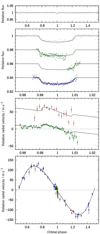
From periodic dimmings seen in their SuperWASP-North and WASP-South lightcurves (Pollacco et al. 2006; top panel of Figs. 1 to 4), we identified each star as a candidate host of a transiting planet using the techniques described
inCollier Cameron et al.(2006,2007). We conducted
pho-tometric and spectroscopic follow-up observations using var-ious facilities at the ESO La Silla observatory: the EulerCam imager and the CORALIE spectrograph, both mounted on the 1.2-m Swiss Euler telescope (Lendl et al. 2012;Queloz et al. 2000), the 0.6-m TRAPPIST-South imager (Gillon et al.
2011;Jehin et al. 2011), and the HARPS-S spectrograph on
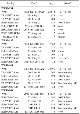
the 3.6-m ESO telescope (Pepe et al. 2002). We obtained ad-ditional data using the HARPS-N spectrograph on the 3.6-m Telescopio Nazionale Galileo at the Observatorio del Roque de los Muchachos (Cosentino et al. 2012). We provide a summary of our observations in Table1.
We obtained lightcurves from the time-series images using standard differential aperture photometry (second panel of Figs. 1 to4). We computed radial-velocity (RV) measure-ments from the CORALIE and HARPS spectra by weighted cross-correlation with a G2 binary mask (Baranne et al.
1996;Pepe et al. 2002). We detected sinusoidal variations in
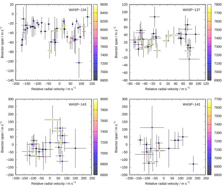
the RVs with semi-amplitudes consistent with planetary mass companions and that phase with the WASP ephemerides (bottom panel of Figs. 1to4). The lack of correlation
be-0.95 1 1.05 0.6 0.8 1 1.2 1.4 Relative flux 0.95 1 1.05 0.6 0.8 1 1.2 1.4 0.92 0.94 0.96 0.98 1 0.98 0.99 1 1.01 1.02 Relative flux 0.92 0.94 0.96 0.98 1 0.98 0.99 1 1.01 1.02 −50 0 50 0.98 0.99 1 1.01 1.02
Relative radial velocity / m s
−1 −50 0 50 0.98 0.99 1 1.01 1.02 −150 −100 −50 0 50 100 150 0.6 0.8 1 1.2 1.4
Relative radial velocity / m s
−1 Orbital phase −150 −100 −50 0 50 100 150 0.6 0.8 1 1.2 1.4
Figure 1. WASP-134b discovery data. Top panel: WASP lightcurve folded on the transit ephemeris and binned with a bin width of 10 min. Second panel: Transit lightcurves from WASP (grey), TRAPPIST-South (green) and EulerCam (blue), offset for clarity, binned with a bin width of 2 min (10 min for WASP), and plotted chronologically with the most recent lightcurve at the bottom. The best-fitting transit model is superimposed. Third panel: The RVs from HARPS-S (brown) and HARPS-N (green) showing the ap-parent anomaly during transit, along with the best-fitting Rossiter-McLaughlin (RM) effect model. Bottom panel: The RVs from CORALIE (blue), HARPS-S and HARPS-N, with the best-fitting eccentric orbital model. WASP-134 reached high airmass by the end of each photometric and spectroscopic transit sequence.
Table 1. Summary of observations
Facility Datea N
obs Notesb WASP-134
WASP 2008 Jun–2010 Oct 28 614 400–700 nm TRAPPIST-South 2014 Sep 05 678 I + z TRAPPIST-South 2014 Oct 26 284 I + z Euler/EulerCam 2016 Sep 25 338 NGTS filter Euler/CORALIE 2014 Jul–2018 Oct 33 orbit ESO3.6/HARPS-S 2015 Jun–2015 Aug 10 orbit ESO3.6/HARPS-S 2015 Aug 16 17 transit TNG/HARPS-N 2018 Aug 16 47 transit WASP-137
WASP 2008 Jul–2010 Dec 17 463 400–700 nm TRAPPIST-South 2014 Nov 10 577 I + z Euler/EulerCam 2014 Nov 14 303 Gunn r TRAPPIST-South 2014 Dec 27 709 I + z TRAPPIST-South 2015 Sep 03 982 I + z; MF Euler/CORALIE 2014 Sep–2017 Jan 32 orbit WASP-143
WASP 2009 Jan–2012 Apr 32 995 400–700 nm TRAPPIST-South 2015 Jan 31 767 blue-blocking Euler/EulerCam 2015 Feb 15 199 NGTS filter Euler/EulerCam 2015 Mar 06 178 NGTS filter TRAPPIST-South 2016 Feb 09 843 blue-blocking; MF Euler/CORALIE 2014 Feb–2017 May 22 orbit
WASP-146
WASP 2008 Jun–2011 Nov 54 839 400–700 nm Euler/EulerCam 2014 Nov 18 190 NGTS filter TRAPPIST-South 2014 Nov 18 791 blue-blocking Euler/EulerCam 2015 Jul 17 150 NGTS filter TRAPPIST-South 2015 Jul 17 874 blue-blocking; MF Euler/CORALIE 2014 Jul–2016 Oct 16 orbit
a The dates are ‘night beginning’.
b For the photometry datasets, we state which filter was used. For the spec-troscopy datasets, we indicate whether the data cover the orbit or the transit. ‘MF’ indicates that TRAPPIST-South performed a meridian flip, which was accounted for by including an offset during lightcurve fitting.
tween RV and bisector span supports our conclusion that the RV signals are induced by orbiting bodies and not by stellar activity (Fig.5;Queloz et al. 2001).
3. STELLAR ANALYSIS
We performed spectral analyses using the procedures de-tailed in Doyle et al. (2013) to obtain stellar effective tem-perature Teff, surface gravity log g∗, metallicity [Fe/H], pro-jected rotation speed v sin i∗,spec, and lithium abundance log A(Li). The results of the spectral analyses are given in Table 2. We calculated macroturbulence using the cali-bration ofDoyle et al.(2014). We calculated distance using the Gaia DR2 parallax (Gaia Collaboration et al. 2018), and stellar luminosity and radius using the infrared flux method (IRFM) of Blackwell & Shallis (1977). Using the method
ofMaxted et al. (2011), we checked for modulation of the
WASP lightcurves as can be caused by the combination of
0.95 1 1.05 0.4 0.6 0.8 1 1.2 1.4 1.6 Relative flux 0.95 1 1.05 0.4 0.6 0.8 1 1.2 1.4 1.6 0.9 0.92 0.94 0.96 0.98 1 1.02 0.96 0.98 1 1.02 1.04 Relative flux 0.9 0.92 0.94 0.96 0.98 1 1.02 0.96 0.98 1 1.02 1.04 −100 −50 0 50 100 0.4 0.6 0.8 1 1.2 1.4 1.6
Relative radial velocity / m s
−1 Orbital phase −100 −50 0 50 100 0.4 0.6 0.8 1 1.2 1.4 1.6
Figure 2. WASP-137b discovery data. As for Fig.1. The meridian flip is indicated with a vertical dashed line.
magnetic activity and stellar rotation. We find no signals with amplitudes greater than 1–2 mmag.
Though we can measure stellar density ρ∗directly from the transit lightcurves, we require a constraint on stellar mass M∗ or radius R∗for a full characterisation of the system. For each star we inferred M∗and age τ using the bagemass stellar evo-lution MCMC code ofMaxted et al.(2015), with input of the values of ρ∗from initial MCMC analyses (see Section2) and Teffand [Fe/H] from the spectral analyses. We conservatively inflated the error bar by a factor of 2 to place Gaussian priors on M∗in our final MCMC analyses. We note that the values of R∗from our final MCMC analyses are consistent with the values obtained from the IRFM and the Gaia parallax (com-pare the values in Tables2and4).
sectionSystem parameters from MCMC analyses We de-termined the system parameters from a simultaneous fit to the transit lightcurves and the radial velocities using the current version of the Markov-chain Monte Carlo (MCMC) code
Table 2. Stellar parameters
Parameter Symbol WASP-134 WASP-137 WASP-143 WASP-146 Unit
Constellation . . . Pegasus Cetus Hydra Aquarius . . .
Right Ascension (J2000) . . . 21h50m16.s77 01h43m29.s09 09h23m22.s96 23h56m22.s02 . . . Declination (J2000) . . . +04◦11′40.s3 −14◦08′56.s8 +02◦55′57.s1 −13◦16′17.s6 . . . Tycho-2 Vmag V 11.3 11.0 12.6a 12.9a . . . 2MASS Kmag K 9.4 9.5 11.3 11.0 . . . Spectral typeb . . . G4 G0 G1 G0 . . .
Stellar effective temperature Teff 5700 ± 100 6100 ± 140 5900 ± 140 6100 ± 140 K
Distance (Gaia) d 195 ± 2 289 ± 4 402 ± 7 495 ± 27 pc
Stellar mass M∗ 1.131 ± 0.045 1.216 ± 0.066 1.087 ± 0.045 1.057 ± 0.085 M⊙ Stellar radius (IRFM) R∗,IRFM 1.16 ± 0.06 1.65 ± 0.10 1.00 ± 0.05 1.29 ± 0.06 R⊙ Stellar surface gravity log g∗ 4.4 ± 0.1 4.0 ± 0.2 4.4 ± 0.2 4.3 ± 0.2 [cgs] Stellar metallicityc [Fe/H] +0.40 ± 0.07 +0.08 ± 0.07 +0.23 ± 0.10
−0.01 ± 0.16 . . . Stellar luminosity log(L/L⊙) 0.103 ± 0.048 0.487 ± 0.051 0.027 ± 0.041 0.268 ± 0.044 . . . Proj. stellar rotation speed vsin i∗,spec 0.9 ± 0.6 3.7 ± 0.9 0.9 ± 0.9 0.9 ± 0.9 km s−1 Lithium abundance log A(Li) <0.4 2.87 ± 0.08 <1.6 <1.6 . . . Macroturbulenced v
mac 3.1 5.0 3.6 3.8 km s−1
Age τ 5.1 ± 1.6 4.3 ± 1.8 1.9 ± 1.5 6.9 ± 2.5 Gyr
a From the USNO YB6 catalog.
b Spectral type estimated using the table inGray(1992).
c Iron abundance is relative to the solar value ofAsplund et al.(2009).
d Macroturbulence from the calibration ofDoyle et al.(2014), with an error of 0.7 km s−1.
presented in Collier Cameron et al. (2007) and described further in Anderson et al. (2015b). We partitioned those TRAPPIST-South lightcurves affected by meridian flips so as to account for any offsets. When fitting eccentric orbits, we obtained e = 0.076±0.032 for WASP-137b, e = 0.0021+0.0014 −0.0007 for WASP-143b, and e = 0.041+0.049−0.029for WASP-146b. Each value is small and of low significance, so we adopted circu-lar orbits, as is encouraged byAnderson et al.(2012) for hot Jupiters in the absence of evidence to the contrary.
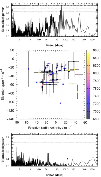
We adopted an eccentric orbit for WASP-134b (P = 10.1 d) as it fits the data much better than does a circular orbit (∆AICc = 40). Having noticed excess scatter about an initial fit, we calculated a periodogram of the residuals and found a significant peak around P = 70 d (Fig.6, top panel; FAP < 0.001), which we attribute to the planet WASP-134c. The ab-sence of a correlation between bisector span and residual RV (about the best-fitting orbit for WASP-134b) supports our in-terpretation that the 70-d signal is induced by a planet and not stellar activity (Fig.6, middle panel). We used the RadVel code ofFulton et al.(2018) to fit a two-planet model, fixing P and Tcfor the inner planet at the values derived from the tran-sit photometry, placing a limit on eccentricity of e < 0.35, and excluding the transit sequences. We plot the best-fitting two-planet model in Fig.7and provide the two-planet solu-tion in Table 3. The two-planet model is a much better fit to the data than is the one-planet model (∆AICc = 111). A periodogram of the residual RVs about the two-planet model shows no significant peak (Fig.6, bottom panel). We do not
Table 3. Two-planet solution for WASP-134
Parameter Symbol WASP-134b WASP-134c Unit Orbital period P 10.1498 (fixed) 70.01 ± 0.14 d Epoch of infer. conjunc. Tconj 2457464.848 (fixed) 2457234.2 ± 1.8 d Orbital eccentricity e 0.146 ± 0.015 0.173 ± 0.090 . . . Arg. of periastron ω −97.2 ± 2.6 58 ± 32 ◦ Refl. veloc. semi-ampl. K1 122.1 ± 2.1 32.5 ± 2.7 km s−1 Minimum planet mass MPsin i 1.40 ± 0.08 0.70 ± 0.07 MJup
see evidence of transits of WASP-134c in the WASP data, but the phase coverage is sparse (only a few transits of WASP-134b had good coverage). TESS is scheduled to observe WASP-134 during 2019 Aug 15 to 2019 Sep 11 (camera 1, Sector 15), whereas we predict the nearby inferior conjunc-tions of WASP-134c to occur on 2019 Aug 8 and 2019 Oct 17, with a 1-σ uncertainty of 5 d. We subtracted the best-fitting orbit of WASP-134c from the RVs of WASP-134 prior to the MCMC analysis.
For each system, to for instrumental and astrophysical off-sets, we partitioned the RV datasets and fit a separate sys-temic velocity to each of them. This included the CORALIE RVs from before and after the November 2014 upgrade (la-belled CORALIE07 and CORALIE14, respectively), and the HARPS RVs around the orbit and through the transits of WASP-134b.
0.95 1 1.05 0.4 0.6 0.8 1 1.2 1.4 1.6 Relative flux 0.95 1 1.05 0.4 0.6 0.8 1 1.2 1.4 1.6 0.9 0.92 0.94 0.96 0.98 1 0.96 0.98 1 1.02 1.04 Relative flux 0.9 0.92 0.94 0.96 0.98 1 0.96 0.98 1 1.02 1.04 −150 −100 −50 0 50 100 150 0.4 0.6 0.8 1 1.2 1.4 1.6
Relative radial velocity / m s
−1 Orbital phase −150 −100 −50 0 50 100 150 0.4 0.6 0.8 1 1.2 1.4 1.6
Figure 3. WASP-143b discovery data. As for Fig.2.
For WASP-134b, we modelled the Rossiter-McLaughlin (RM) effect using the formulation of Hirano et al. (2011). Due to the low transit impact parameter, there is a degeneracy between the projected stellar rotation speed v sin i∗,RMand the projected stellar obliquity λ (e.g.Albrecht et al. 2011). This results in values of v sin i∗,RM(> 9 km s−1) far higher than the value from our spectral analysis (v sin i∗,spec = 0.9 ± 0.6 km s−1), so we placed a Gaussian prior on v sin i
∗,RMusing the value from the spectral analysis. With the prior, we obtained λ = −43.7 ± 9.9◦and v sin i
∗,RM=2.08 ± 0.26 km s−1. With-out the prior, we obtained λ = −67+15
−9
◦ and v sin i ∗,RM = 3.3+1.5−0.9km s−1.
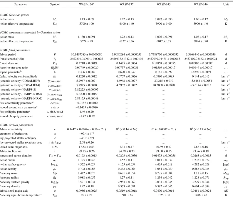
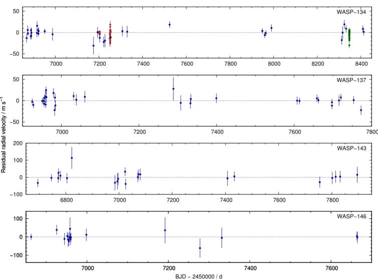
We present the median values and 1-σ limits on the sys-tem parameters from our final MCMC analyses in Table4. We plot the best fits to the RVs and the transit lightcurves in Figs.1to4and the residuals of the RVs about the best-fitting orbital models in Fig.8.
0.95 1 1.05 0.4 0.6 0.8 1 1.2 1.4 1.6 Relative flux 0.95 1 1.05 0.4 0.6 0.8 1 1.2 1.4 1.6 0.9 0.92 0.94 0.96 0.98 1 0.96 0.98 1 1.02 1.04 Relative flux 0.9 0.92 0.94 0.96 0.98 1 0.96 0.98 1 1.02 1.04 −200 −100 0 100 200 0.4 0.6 0.8 1 1.2 1.4 1.6
Relative radial velocity / m s
−1 Orbital phase −200 −100 0 100 200 0.4 0.6 0.8 1 1.2 1.4 1.6
Figure 4. WASP-146b discovery data. As for Fig.2.
4. DISCUSSION
We have presented the discovery of five Jupiter-mass plan-ets (MP=0.68–1.41 MJup) orbiting moderately bright (V = 11.0–12.9) Solar-type stars (M∗=1.06–1.22 M⊙). As fairly typical hot Jupiters (Teql=1300–1600 K) with orbital periods of P = 3–4 d, WASP-137b, WASP-143b and WASP-146b are remarkably similar to each other (Tables2and4).
The 134 system is rather more interesting. WASP-134 is a metal-rich G4 star ([Fe/H] = +0.40 ± 0.07) orbited by two warm Jupiters. WASP-134b (MP =1.41 MJup; Teql =950 K) is in an eccentric (e = 0.15 ± 0.01), 10.15-d orbit (a = 0.096 AU) that is misaligned with the spin of the star (λ = −44 ± 10◦). Its companion, WASP-134c (MP sin i = 0.70 MJup; Teql=500 K), is in an eccentric (e = 0.17 ± 0.09), 70.0-d orbit (a = 0.35 AU). Thus WASP-134 is a rare type of system: a hot/warm Jupiter with a nearby giant companion. In that respect, WASP-134 may be similar to the HAT-P-46 system. Hartman et al.(2014) found that their RVs of HAT-P-46 are fit well with a two-planet model: MP=0.49 and P =
Table 4. System parameters
Parameter Symbol WASP-134a WASP-137 WASP-143 WASP-146 Unit
MCMC Gaussian priors
Stellar mass M∗ 1.13 ± 0.09 1.22 ± 0.13 1.087 ± 0.090 1.06 ± 0.17 M⊙
Stellar effective temperature Teff 5700 ± 100 6100 ± 140 5900 ± 1400 5900 ± 140 K
MCMC parameters controlled by Gaussian priors
Stellar mass M∗ 1.130 ± 0.091 1.22 ± 0.13 1.096 ± 0.091 1.06 ± 0.17 M⊙
Stellar effective temperature Teff 5574 ± 99 6127 ± 136 6042 ± 135 5894 ± 140 K
MCMC fitted parameters
Orbital period P 10.1467583 ± 0.0000080 3.9080284 ± 0.0000053 3.7788730 ± 0.0000032 3.3969440 ± 0.0000036 d Transit epoch (HJD) Tc 2457201.03099 ± 0.00075 2456937.61342 ± 0.00106 2457099.94471 ± 0.00015 2457109.72182 ± 0.00021 d Transit duration T14 0.2218 ± 0.0019 0.1425 ± 0.0034 0.12858 ± 0.00055 0.09980 ± 0.00097 d Planet-to-star area ratio R2
P/R 2
∗ 0.00749 ± 0.00020 0.00737 ± 0.00031 0.01569 ± 0.00017 0.01049 ± 0.00017 . . .
Impact parameterb b 0.306 ± 0.082 0.690 ± 0.049 0.181 ± 0.097 0.8290 ± 0.0089 . . .
Reflex velocity semi-amplitude K1 0.1220 ± 0.0012 0.0767 ± 0.0026 0.0890 ± 0.0085 0.144 ± 0.012 km s−1 Systemic velocity (CORALIE07) γCORALIE07 5.7967 ± 0.0021 4.6948 ± 0.0027 20.215 ± 0.010 −5.6464 ± 0.0084 km s−1 Systemic velocity (CORALIE14) γCORALIE14 5.7975 ± 0.0020 4.6937 ± 0.0022 20.2008 ± 0.0088 −5.6144 ± 0.015 km s−1
Systemic velocity (HARPS-S) γHARPS−S 5.82223 ± 0.00097 . . . km s−1
Systemic velocity (HARPS-S RM) γHARPS−SRM 5.8200 ± 0.0015 . . . km s−1
Systemic velocity (HARPS-N RM) γHARPS−NRM 5.83155 ± 0.00048 . . . km s−1
First eccentricity parameterc ecos ω
−0.0187 ± 0.0042 . . . .
Second eccentricity parameterc esin ω
−0.1435 ± 0.0086 . . . .
First obliquity parameterc v
∗sin i∗cos λ 1.49 ± 0.20 . . . .
Second obliquity parameterc v
∗sin i∗sin λ −1.42 ± 0.39 . . . .
MCMC derived parameters
Orbital eccentricity e 0.1447 ± 0.0086 (< 0.16 at 2σ) 0d(< 0.14 at 2σ) 0d(< 0.0007 at 2σ) 0d(< 0.15 at 2σ) . . .
Argument of periastron ω −97.4 ± 1.7 . . . ◦
Sky-projected stellar obliquity λ −43.7 ± 9.9 . . . ◦
Sky-projected stellar rotation speed vsin i∗,RM 2.08 ± 0.26 . . . km s−1
Scaled semi-major axis a/R∗ 17.53 ± 0.53 7.31 ± 0.47 10.39 ± 0.17 7.88 ± 0.16 . . .
Orbital inclination i 89.13 ± 0.26 84.59 ± 0.73 89.00 ± 0.55 83.96 ± 0.19 ◦
Ingress and egress duration T12= T34 0.0193 ± 0.0013 0.0203 ± 0.0030 0.01473 ± 0.00056 0.0263 ± 0.0015 d
Stellar radius R∗ 1.175 ± 0.048 1.52 ± 0.11 1.013 ± 0.032 1.232 ± 0.072 R⊙
Stellar surface gravity log g∗ 4.352 ± 0.029 4.155 ± 0.059 4.465 ± 0.018 4.282 ± 0.029 [cgs]
Stellar density ρ∗ 0.702 ± 0.063 0.343 ± 0.066 1.054 ± 0.050 0.568 ± 0.035 ρ⊙
Planetary mass MP 1.412 ± 0.075 0.681 ± 0.054 0.725 ± 0.084 1.11 ± 0.15 MJup
Planetary radius RP 0.988 ± 0.057 1.27 ± 0.11 1.234 ± 0.042 1.228 ± 0.076 RJup
Planetary surface gravity log gP 3.521 ± 0.034 2.983 ± 0.069 3.033 ± 0.045 3.229 ± 0.044 [cgs]
Planetary density ρP 1.47 ± 0.18 0.333 ± 0.081 0.382 ± 0.045 0.604 ± 0.084 ρJ
Orbital semi-major axis a 0.0956 ± 0.0025 0.0519 ± 0.0018 0.0490 ± 0.0014 0.0451 ± 0.0024 AU Planetary equilibrium temperaturee T
eql 953 ± 22 1601 ± 65 1325 ± 30 1486 ± 43 K
a These values are for WASP-134b. For the values relating to WASP-134c, see Table3.
b Impact parameter is the distance between the centre of the stellar disc and the transit chord: b = a cos i/R∗.
c We actually fit √e cos ω, √e sin ω, √v∗sin i∗cos λ and√v∗sin i∗sin λ, but we give these quantities for ease of interpretation and comparison with other studies.
d We assumed circular orbits for these systems.
−140 −120 −100 −80 −60 −40 −20 0 20 −200 −150 −100 −50 0 50 100 150 WASP−134 Bisector span / m s −1
Relative radial velocity / m s−1
6800 7000 7200 7400 7600 7800 8000 8200 8400 8600 −80 −60 −40 −20 0 20 40 60 80 100 120 −80 −60 −40 −20 0 20 40 60 80 100 120 WASP−137 Bisector span / m s −1
Relative radial velocity / m s−1
6900 7000 7100 7200 7300 7400 7500 7600 7700 7800 −200 −150 −100 −50 0 50 100 150 200 250 300 −200 −150 −100 −50 0 50 100 150 200 250 WASP−143 Bisector span / m s −1
Relative radial velocity / m s−1
6600 6800 7000 7200 7400 7600 7800 8000 −200 −150 −100 −50 0 50 100 150 200 250 300 −200 −150 −100 −50 0 50 100 150 200 250 WASP−143 Bisector span / m s −1
Relative radial velocity / m s−1
6800 6900 7000 7100 7200 7300 7400 7500 7600 7700
Figure 5. Bisector span versus radial velocity. The colour bar depicts the Barycentric Julian Date (BJD-2450000). For WASP-134, we omit the HARPS data taken through the transits as they will be affected by the RM effect.
10.0 100.0 1000. 2. 5. 20. 50. 200. 500. 0.0 0.1 0.2 0.3 0.4 0.5 Period [days] Normalized power . . . . −140 −120 −100 −80 −60 −40 −20 0 20 −80 −60 −40 −20 0 20 40 60 Bisector span / m s −1
Relative radial velocity / m s−1
6800 7000 7200 7400 7600 7800 8000 8200 8400 8600 10.0 100.0 1000. 2. 5. 20. 50. 200. 500. 0.0 0.1 0.2 0.3 0.4 Period [days] Normalized power . . . .
Figure 6. The evidence for WASP-134c. Top panel: The pe-riodogram of the residual RVs of WASP-134 after subtraction of the motion due to WASP-134b (P = 10.15 d). The horizontal lines indicate the 10, 1 and 0.1 per cent false-alarm levels. The peak around 70 d, which we attribute to the planet WASP-134c, has a false-alarm probability of FAP < 0.001. Middle panel: Bisector span versus residual RV of WASP-134 after subtraction of the mo-tion due to WASP-134b. The colour bar depicts the Barycentric Julian Date (BJD-2450000). Bottom panel: The periodogram of the residual RVs of WASP-134 after subtraction of the motion due to both WASP-134b and WASP-134c (P = 70.0 d).
4.5 d for HAT-P-46b and MPsin i = 2.0 MJupand P = 78 d for the candidate planet 46c. The evidence for HAT-P-46c, though, is not yet conclusive and further RV monitoring is required.
Of those hot/warm Jupiters with confirmed giant compan-ions, the companions tend to be very far out (e.g. HAT-P-17c with P = 1610 d; Howard et al. 2012), and rarely
Figure 7. A two-planet fit to the RVs of WASP-134 (exclud-ing the transit sequences). Top panel: The phase-folded orbit of WASP-134b (P = 10.15 d). Bottom panel: The phase-folded orbit of WASP-134c (P = 70.0 d). The CORALIE07 and CORALIE14 RVs are shown as yellow circles and red stars, respectively. The HARPS-S RVs are shown as green diamonds.
closer than 1 AU (e.g. WASP-41c at a = 1.07 AU and WASP-47c at a = 1.36 AU; Neveu-VanMalle et al. 2016). Also of note are those hot-Jupiter systems with brown-dwarf companions within a few AU, such as WASP-53 and WASP-81 (Triaud et al. 2017). In their tabulation of hot and warm Jupiters with nearby giant companions,Antonini et al. (2016) list only three companions inside of 1 AU, the clos-est of which is HD 9446 c at 0.65 AU (H´ebrard et al. 2010). With a = 0.35 AU, WASP-134c is in a much shorter orbit.
It seems unlikely that WASP-134b could have arrived in situ via high-eccentricity migration (e.gPetrovich & Tremaine
2016). Antonini et al.(2016) studied the observed
popula-tion of hot and warm Jupiters with nearby giant companions and found that the ejection of a planet or its collision with the star are more likely outcomes when exploring such path-ways. Thus in-situ formation (e.g.Huang et al. 2016) or disc migration (e.g. Lin et al. 1996) seem more likely explana-tions.
SuperWASP-North is hosted by the Issac Newton Group on La Palma and WASP-South is hosted by SAAO; we are grateful for their support and assistance. Funding for WASP comes from consortium universities and from the UK’s Sci-ence and Technology Facilities Council. The Swiss Euler Telescope is operated by the University of Geneva, and is funded by the Swiss National Science Foundation. The re-search leading to these results has received funding from the ARC grant for Concerted Research Actions, financed by the Wallonia-Brussels Federation. TRAPPIST is funded
−50 0 50 7000 7200 7400 7600 7800 8000 8200 8400 WASP−134 −50 0 50 7000 7200 7400 7600 7800 WASP−137 −100 0 100 200 6800 7000 7200 7400 7600 7800 WASP−143 −100 0 100 7000 7200 7400 7600 WASP−146
Residual radial velocity / m s
−1
−100 0 100
7000 7200 7400 7600
Residual radial velocity / m s
−1
BJD − 2450000 / d
Figure 8. The residual RVs about the best-fitting orbital and RM effect models. The symbol colours are the same as in Fig.1.
by the Belgian Fund for Scientific Research (Fond National de la Recherche Scientifique, FNRS) under the grant FRFC 2.5.594.09.F, with the participation of the Swiss National Science Foundation (SNF). MG and EJ are FNRS Senior Re-search Associates. Based on observations collected at the Eu-ropean Organisation for Astronomical Research in the South-ern Hemisphere under ESO programmes 095.C-0105(A) and 097.C-0434(B). Based on observations under programme CAT18A 138 made with the Italian Telescopio Nazionale Galileo (TNG) operated on the island of La Palma by the
Fundaci´on Galileo Galilei of the INAF (Istituto Nazionale di Astrofisica) at the Spanish Observatorio del Roque de los Muchachos of the Instituto de Astrofisica de Canarias. This research has made use of TEPCat, a catalogue of the physi-cal properties of transiting planetary systems maintained by John Southworth.
Facilities:
SuperWASP (SuperNorth, WASP-South), TRAPPIST, Euler1.2m (CORALIE, EulerCam), ESO:3.6m (HARPS-S), TNG (HARPS-N)REFERENCES
Albrecht, S., Winn, J. N., Johnson, J. A., et al. 2011, ApJ, 738, 50, doi:10.1088/0004-637X/738/1/50
Anderson, D. R., Collier Cameron, A., Gillon, M., et al. 2012, MNRAS, 422, 1988, doi:10.1111/j.1365-2966.2012.20635.x
Anderson, D. R., Triaud, A. H. M. J., Turner, O. D., et al. 2015a, ApJL, 800, L9, doi:10.1088/2041-8205/800/1/L9
Anderson, D. R., Collier Cameron, A., Hellier, C., et al. 2015b, A&A, 575, A61, doi:10.1051/0004-6361/201423591
Antonini, F., Hamers, A. S., & Lithwick, Y. 2016, AJ, 152, 174, doi:10.3847/0004-6256/152/6/174
Asplund, M., Grevesse, N., Sauval, A. J., & Scott, P. 2009, ARA&A, 47, 481,
Bakos, G. ´A. 2018, The HATNet and HATSouth Exoplanet Surveys, 111
Baranne, A., Queloz, D., Mayor, M., et al. 1996, A&AS, 119, 373 Becker, J. C., Vanderburg, A., Adams, F. C., Rappaport, S. A., &
Schwengeler, H. M. 2015, ApJL, 812, L18, doi:10.1088/2041-8205/812/2/L18
Blackwell, D. E., & Shallis, M. J. 1977, MNRAS, 180, 177 Broeg, C., Fortier, A., Ehrenreich, D., et al. 2013, in European
Physical Journal Web of Conferences, Vol. 47, European Physical Journal Web of Conferences, 03005
Collier Cameron, A., Pollacco, D., Street, R. A., et al. 2006, MNRAS, 373, 799, doi:10.1111/j.1365-2966.2006.11074.x
Collier Cameron, A., Wilson, D. M., West, R. G., et al. 2007, MNRAS, 380, 1230, doi:10.1111/j.1365-2966.2007.12195.x
Cooke, B. F., Pollacco, D., West, R., McCormac, J., & Wheatley, P. J. 2018, A&A, 619, A175,
doi:10.1051/0004-6361/201834014
Cosentino, R., Lovis, C., Pepe, F., et al. 2012, in Society of Photo-Optical Instrumentation Engineers (SPIE) Conference Series, Vol. 8446, Society of Photo-Optical Instrumentation Engineers (SPIE) Conference Series
Delrez, L., Gillon, M., Queloz, D., et al. 2018, in Society of Photo-Optical Instrumentation Engineers (SPIE) Conference Series, Vol. 10700, Ground-based and Airborne Telescopes VII, 107001I
Doyle, A. P., Davies, G. R., Smalley, B., Chaplin, W. J., & Elsworth, Y. 2014, MNRAS, 444, 3592,
doi:10.1093/mnras/stu1692
Doyle, A. P., Smalley, B., Maxted, P. F. L., et al. 2013, MNRAS, 428, 3164, doi:10.1093/mnras/sts267
Fulton, B. J., Petigura, E. A., Blunt, S., & Sinukoff, E. 2018, PASP, 130, 044504, doi:10.1088/1538-3873/aaaaa8
Gaia Collaboration, Brown, A. G. A., Vallenari, A., et al. 2018, A&A, 616, A1, doi:10.1051/0004-6361/201833051
Gillon, M., Jehin, E., Magain, P., et al. 2011, Detection and Dynamics of Transiting Exoplanets, St. Michel l’Observatoire, France, Edited by F. Bouchy; R. D´ıaz; C. Moutou; EPJ Web of Conferences, Volume 11, id.06002, 11, 6002,
doi:10.1051/epjconf/20101106002
Gray, D. F. 1992, The observation and analysis of stellar photospheres.
Hartman, J. D., Bakos, G. ´A., Torres, G., et al. 2014, AJ, 147, 128, doi:10.1088/0004-6256/147/6/128
H´ebrard, G., Bonfils, X., S´egransan, D., et al. 2010, A&A, 513, A69, doi:10.1051/0004-6361/200913790
Hellier, C., Anderson, D. R., Collier Cameron, A., et al. 2012, MNRAS, 426, 739, doi:10.1111/j.1365-2966.2012.21780.x
Hirano, T., Suto, Y., Winn, J. N., et al. 2011, ApJ, 742, 69, doi:10.1088/0004-637X/742/2/69
Howard, A. W., Bakos, G. ´A., Hartman, J., et al. 2012, ApJ, 749, 134, doi:10.1088/0004-637X/749/2/134
Huang, C., Wu, Y., & Triaud, A. H. M. J. 2016, ApJ, 825, 98, doi:10.3847/0004-637X/825/2/98
Jehin, E., Gillon, M., Queloz, D., et al. 2011, The Messenger, 145, 2
Lendl, M., Anderson, D. R., Collier-Cameron, A., et al. 2012, A&A, 544, A72, doi:10.1051/0004-6361/201219585
Lin, D. N. C., Bodenheimer, P., & Richardson, D. C. 1996, Nature, 380, 606, doi:10.1038/380606a0
Maxted, P. F. L., Serenelli, A. M., & Southworth, J. 2015, A&A, 575, A36, doi:10.1051/0004-6361/201425331
Maxted, P. F. L., Anderson, D. R., Collier Cameron, A., et al. 2011, PASP, 123, 547, doi:10.1086/660007
Neveu-VanMalle, M., Queloz, D., Anderson, D. R., et al. 2016, A&A, 586, A93, doi:10.1051/0004-6361/201526965
Pepe, F., Mayor, M., Rupprecht, G., et al. 2002, The Messenger, 110, 9
Pepper, J., Pogge, R. W., DePoy, D. L., et al. 2007, PASP, 119, 923, doi:10.1086/521836
Petrovich, C., & Tremaine, S. 2016, ApJ, 829, 132, doi:10.3847/0004-637X/829/2/132
Pollacco, D. L., Skillen, I., Cameron, A. C., et al. 2006, PASP, 118, 1407, doi:10.1086/508556
Queloz, D., Mayor, M., Weber, L., et al. 2000, A&A, 354, 99 Queloz, D., Henry, G. W., Sivan, J. P., et al. 2001, A&A, 379, 279,
doi:10.1051/0004-6361:20011308
Ricker, G. R., Winn, J. N., Vanderspek, R., et al. 2014, in Proc. SPIE, Vol. 9143, Space Telescopes and Instrumentation 2014: Optical, Infrared, and Millimeter Wave, 914320 Santerne, A., Moutou, C., Tsantaki, M., et al. 2016, A&A, 587,
A64, doi:10.1051/0004-6361/201527329
Southworth, J. 2011, MNRAS, 417, 2166, doi:10.1111/j.1365-2966.2011.19399.x
Triaud, A. H. M. J., Neveu-VanMalle, M., Lendl, M., et al. 2017, MNRAS, 467, 1714, doi:10.1093/mnras/stx154
Wheatley, P. J., West, R. G., Goad, M. R., et al. 2018, MNRAS, 475, 4476, doi:10.1093/mnras/stx2836
Yao, X., Pepper, J., Gaudi, B. S., et al. 2018, ArXiv e-prints.